Article

Jump and Initial-Sensitive Excessive Motion of a Class of Relative Rotation Systems and Their Control via Delayed Feedback

School of Mechanical Engineering, Shanghai Institute of Technology, Shanghai 201418, China
*
Author to whom correspondence should be addressed.
Mathematics 2022, 10(15), 2676; https://doi.org/10.3390/math10152676
Submission received: 28 June 2022 / Revised: 23 July 2022 / Accepted: 27 July 2022 / Published: 29 July 2022
(This article belongs to the Special Issue Applied Mathematics to Mechanisms and Machines)

Abstract

:
Jump and excessive motion are undesirable phenomena in relative rotation systems, causing a loss of global integrity and reliability of the systems. In this work, a typical relative rotation system is considered in which jump, excessive motion, and their suppression via delayed feedback are investigated. The Method of Multiple Scales and the Melnikov method are applied to analyze critical conditions for bi-stability and initial-sensitive excessive motion, respectively. By introducing the fractal of basins of attraction and the erosion of the safe basin to depict jump and initial-sensitive excessive motion, respectively, the point mapping approach is used to present numerical simulations which are in agreement with the theoretical prediction, showing the validity of the analysis. It is found that jump between bistable attractors can be due to saddle–node bifurcation, while initial-sensitive excessive motion can be due to heteroclinic bifurcation. Under a positive coefficient of the gain, the types of delayed feedback can both be effective in reducing jump and initial-sensitive excessive motion. The results may provide some reference for the performance improvement of rotors and main bearings.

1. Introduction

Rotating machinery, widely used in engineering fields such as transmission systems of vehicles [1] and main bearings of aeroengines [2], plays an important role in the theory of nonlinear dynamics. Due to the nonlinearities of its dynamical systems, it usually undergoes complex dynamics, which have a negative impact on its operational stability and reliability [3,4]. Among these, relative rotation systems have been given much attention, as nonlinear vibration is undesirable. For instance, main shafts can be fatigue damaged by a jump [5,6] among multiple attractors, or by a chaotic response [7], and can even be fractured due to excessive motion [8]. Thus, comprehensive study of the global dynamics of relative rotation systems has become a practical issue.
So far, many researchers have studied the responses of relative rotation systems. Wang et al. [9] obtained the approximate periodic solution of a class of nonlinear systems with relative rotation by applying the Method of Multiple Scales and proved the uniqueness of the periodic response. Xiao et al. [10] verified the existence and uniqueness of periodic response in another type of relative rotation system with a time-varying stiffness. Li et al. [11] proposed a relative rotation system with nonlinear elastic force and nonlinear generalized damping force, and discussed its periodic solution problem theoretically. Shi et al. [12] numerically studied the chaotic behaviors of a relative rotation system under parametric excitation by Poincaré map and maximal Lyapunov exponent. By simulating relative torsional vibrations of an imbalanced shaft under a limited power supply, Verichev [13] found that the interaction of shaft and power supply may result in strange attractors such as classical Lorenz and Feigenbaum attractors. In a nonlinear relative rotation system with a triple-well Mathieu-Duffing oscillator, Liu et al. [14] obtained the threshold of chaos regarding Smale horseshoe commutation and exhibited the erosion process of safe basins. A class of nonlinear relative rotational systems containing two rotors was also built whose chaotic response was presented [15]. By introducing the erosion of the safe basin to describe the safe performance of the spur gear pair, Zhu et al. [16] classified the multiple meshing states and presented the transition process from safe to unsafe. To control the complex dynamics of the main transmission system of a scraper conveyor, Ju et al. [17] analyzed its local bifurcations and proposed a nonlinear state feedback controller whose effect was studied numerically. Considering the effectiveness of time-delay feedback on controlling fractal erosion of the safe basin and chaos in nonlinear dynamical systems [18,19], Zhao et al. [20] applied delayed displacement feedback in a relative torsional vibration system for reducing its response amplitude. On this basis, Shang et al. [21] discussed the effect of delayed position feedback on controlling the erosion of the safe basin and chaos. Although there has been meaningful research on the nonlinear vibration characteristics of the relative rotation system, the study of excessive motion and jump among multiple attractors is mainly carried out by numerical simulation and the mechanism of these complex dynamical behaviors and their control is still not yet clear.
To this end, we select a class of nonlinear relative rotation systems composed of two rotors and study the mechanisms behind its jump and initial-sensitive excessive motion, as well as the effect of delayed feedback on suppressing these phenomena. The paper is arranged as follows. In Section 2, the dynamical model of a relative rotation system is constructed and made dimensionless. In Section 3, the mechanism of jump and excessive motion is analyzed. In Section 4, two control strategies, namely, delay position feedback and delay velocity feedback, are applied to the original system, respectively, whose control mechanism is then discussed. Section 5 contains the discussion.

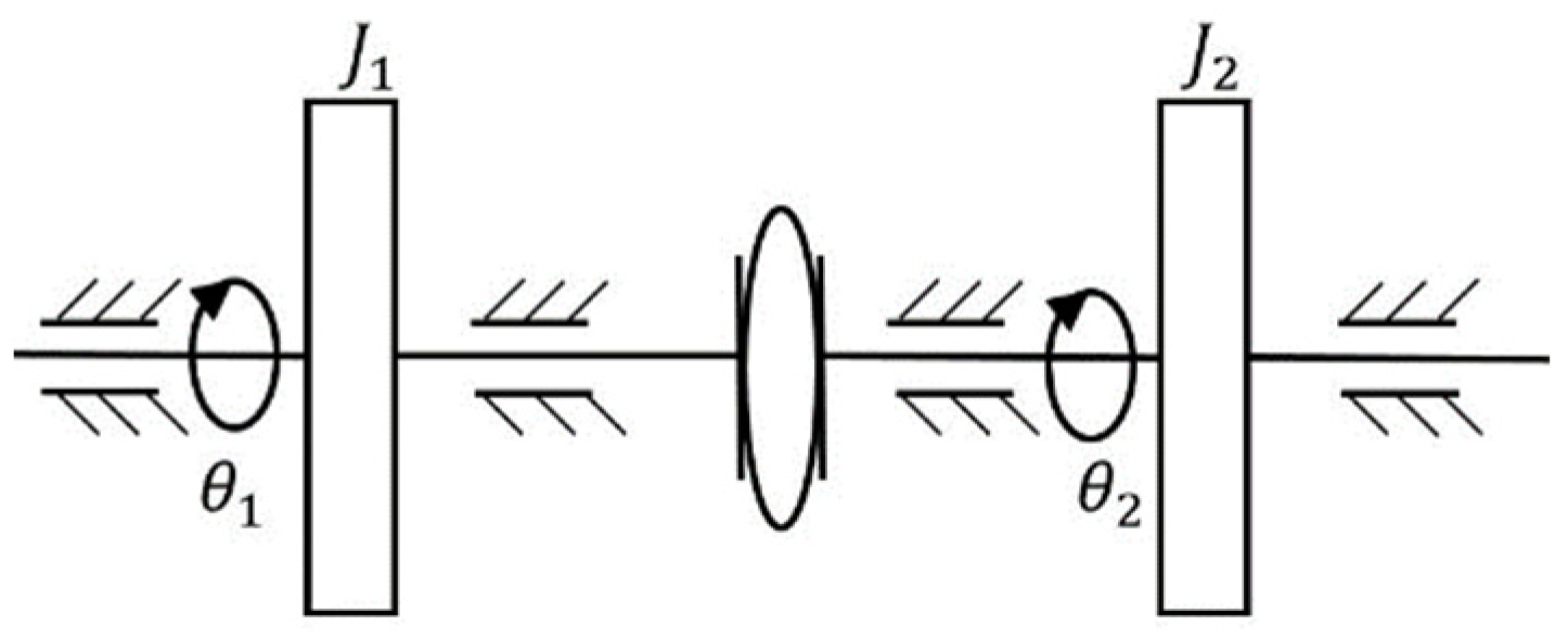
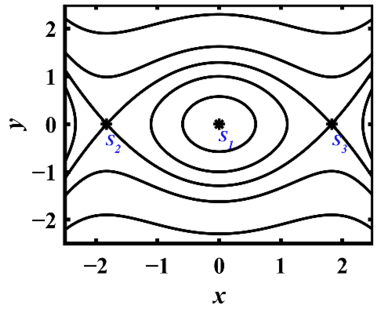
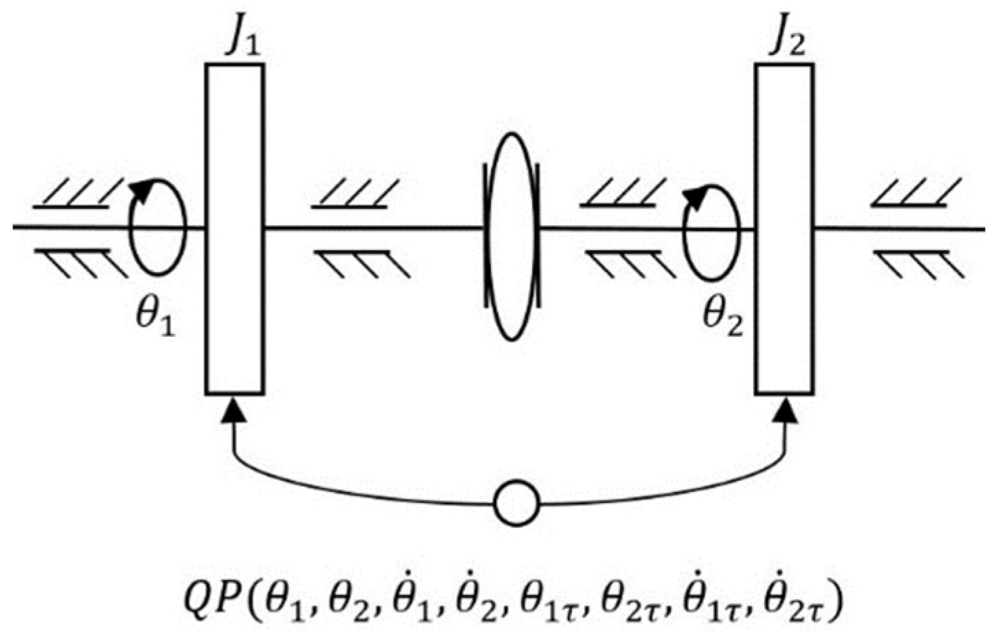
2. Dynamical Model and Unperturbed Dynamics

We consider a typical torsional vibrating system whose simplified diagram is presented in Figure 1. θ 1 and θ 2 are the absolute rotating angles of two rotors, respectively, and J 1 and J 2 represent their polar moments of inertia. Considering nonlinear torsional stiffness and nonlinear damping, the governing equation of this vibrating system can be derived by the momentum theorem as
J 1 θ ¨ 1 + c 12 ( θ ˙ 1 θ ˙ 2 ) + K 1 ( θ 1 θ 2 ) + K 3 ( θ 1 θ 2 ) 3 + f 12 = T e 1 , J 2 θ ¨ 2 + c 12 ( θ ˙ 2 θ ˙ 1 ) + K 1 ( θ 2 θ 1 ) + K 3 ( θ 2 θ 1 ) 3 f 12 = T e 2 ,
where K 1 is the coefficient of linear stiffness between the two rotors; K 3 is the coefficient of nonlinear stiffness satisfying K 3 < 0 ; c 12 is the coefficient of linear damping; T e 1 and T e 2 are external rotational torques loaded on the two rotors, respectively; f 12 is a class of nonlinear stick-slip frictions [20,21] given by
f 12 = c 0 + c 1 ( θ ˙ 1 θ ˙ 2 ) + c 2 ( θ ˙ 1 θ ˙ 2 ) 3 ,
in which c 0 , c 1 and c 2 are the constant of static friction, the coefficient of linear damping and the coefficient of cubic nonlinear damping, respectively. By denoting x = θ 1 θ 2 in Equation (1), the relative rotation system can be obtained as below:
x ¨ + c 12 J 2 + c 12 J 1 J 1 J 2 x ˙ + K 1 ( J 1 + J 2 ) J 1 J 2 x + K 3 ( J 1 + J 2 ) J 1 J 2 x 3 + J 1 + J 2 J 1 J 2 ( c 1 x ˙ + c 2 x ˙ 3 ) = J 2 T e 1 J 1 T e 2 ( J 1 + J 2 ) c 0 J 1 J 2 .
The torques T e 1 and T e 2 are usually harmonic excitations, thus can be represented as
J 2 T e 1 J 1 T e 2 ( J 1 + J 2 ) c 0 J 1 J 2 = F cos ( Ω t )
where F and Ω are the amplitude and the frequency of the excitation, respectively. Introducing the following variables,
ω 0 2 = K 1 ( J 1 + J 2 ) J 1 J 2 , b = K 3 K 1 , μ = ( c 12 + c 1 ) ( J 1 + J 2 ) J 1 J 2 ω 0 , g = c 2 ( J 1 + J 2 ) ω 0 J 1 J 2 , T = ω 0 t , ω = Ω ω 0 , f = F ω 0 2 ,
the dimensionless form of the relative rotation system (3) is obtained as
y = d x d T , d y d T = μ y x + b x 3 g y 3 + f cos ( ω T ) .
in which the parameters μ , b, g, and ω are positive, and the position x ( T ) and the velocity y ( T ) represent relative rotational angular and relative angular velocity at the moment T, respectively.
Since the parameters c 12 , c 0 , c 1 , and c 2 in the original system (1) are very small, the relevant terms concerned, μ , g and f in Equation (6), can be considered as perturbed. The unperturbed system can be written as
d x d T = y , d y d T = x + b x 3 .
There will be three equilibria in the unperturbed system (7), namely, the center S1(0,0) and two saddle points S2( b b ,0) and S3(− b b ,0). The Hamiltonian of Equation (7) is
H ( x , y ) = 1 2 y 2 + 1 2 x 2 1 4 b x 4 .
Accordingly, the heteroclinic orbits surrounding the center S1(0,0) can be given by
x ± ( t ) = ± b b tanh ( 2 2 t ) , y ± ( t ) = ± 2 b 2 b sech 2 ( 2 2 t ) .
Fixing b = 0.3, the unperturbed orbits are depicted in Figure 2.

3. Complex Dynamics

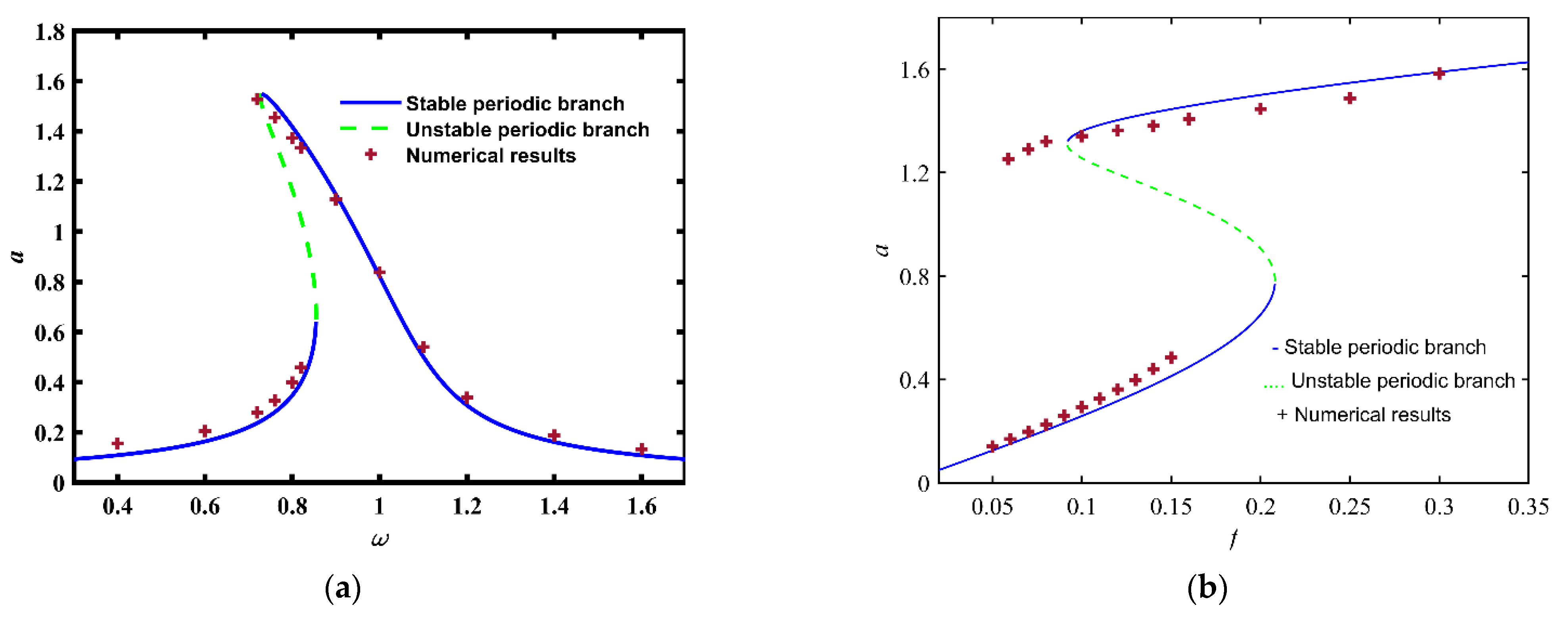
3.1. Multistability and Jump

The periodic solution near the equilibrium S1(0,0) is considered. The Method of Multiple Scales (MMS) [22] is employed to obtain the approximate theoretical solution of Equation (3). Supposing a small parameter ε (0 < ε≪ 1) to rescale the nondimensional parameters as follows:
μ = ε μ ˜ , b = ε b ˜ , g = ε g ˜ , f = ε f ˜ ,
Equation (6) becomes
d 2 x d T 2 + x = ε ( μ ˜ d x d T + b ˜ x 3 g ˜ ( d x d T ) 3 + f ˜ cos ( ω T ) ) .
Further rescaling parameters and operators in Equation (11) yields
ω = 1 + ε σ , T i = ε i T , x ( T ) = x 0 ( T 0 , T 1 , ) + ε x 1 ( T 0 , T 1 , ) + , D i = T i , d d T = i = 0 n ε i D i ( i = 0 , 1 , 2 ) ,
where σ is the detuning parameter, and separating the coefficients of ε 0 and ε 1 of the system (11) one finds
ε 0 : D 0 2 x 0 + x 0 = 0 ,
and
ε 1 : D 0 2 x 1 + x 1 = 2 D 1 D 0 x 0 μ ˜ D 0 x 0 + b ˜ x 0 3 g ˜ ( D 0 x 0 ) 3 + f ˜ cos ( T 0 + σ T 1 ) .
The solution of Equation (13) is
x 0 ( T 0 , T 1 ) = A ( T 1 ) e i T 0 + c c
where cc denotes the complex conjugate of the preceding terms. Substituting Equation (15) into Equation (14) and separating the secular terms yields
D 1 A + μ ˜ A 2 + 3 ( g ˜ + i b ˜ ) A 2 A ¯ 2 + i f ˜ e i σ T 1 4 = 0 .
In addition, by defining
A ( T 1 ) = a ( T 1 ) 2 e i β ( T 1 ) , ψ = σ T 1 β ,
separating the real and imaginary parts of Equation (16), and returning the parameters to the nondimensional parameters of the system (3), the modulation equation can be written as
d a d T = μ a 2 3 g a 3 8 + f sin ψ 2 , a d ψ d T = a ( ω 1 ) + 3 b a 3 8 + f cos ψ 2 .
The steady-state form of Equation (18) is obtained by setting D 1 a = D 1 ψ = 0 and returning the parameters of (18) to the nondimensional parameters as:
μ a + 3 g a 3 4 = f sin ψ , 2 ( ω 1 ) a 3 b a 3 4 = f cos ψ .
Accordingly, the approximate periodic solution can be expressed as x 0 = a cos ( ω T ψ ) . By eliminating ψ from the relationships in Equation (19), its amplitude a can be solved from the following equation
( μ + 3 g a 2 4 ) 2 a 2 + ( 2 ω 2 + 3 4 b a 2 ) 2 a 2 = f 2 .
The corresponding characteristic equation is
( λ + μ 2 + 9 g a 2 8 ) ( λ + μ 2 + 3 g a 2 8 ) + ( ω 1 + 9 8 b a 2 ) ( ω 1 + 3 8 b a 2 ) = 0 ,
meaning that for
27 ( g 2 + b 2 ) 16 a 4 + 3 ( g μ + b ( 2 ω 2 ) ) a 2 + 4 ( ω 1 ) 2 + μ 2 > 0 ,
the periodic solution is unstable and becomes a saddle. Namely, when the inequation (22) becomes an equation, saddle-node bifurcation will occur in the system (6). For
μ = 0.03 , b = 0.3 , g = 0.03 ,
the response curve of Equation (20) is plotted in Figure 3 where the coexistence of two stable periodic branches in the same range of the excitation parameters implies bi-stability. For example, for f = 0.13 and ω within the range (0.65, 0.86), bistable periodic attractors coexist (see Figure 3a). Fixing ω = 0.80, the increase of the amplitude f can also lead to saddle-node bifurcation, and thus bi-stability. The numerical results totally match the theoretical prediction.

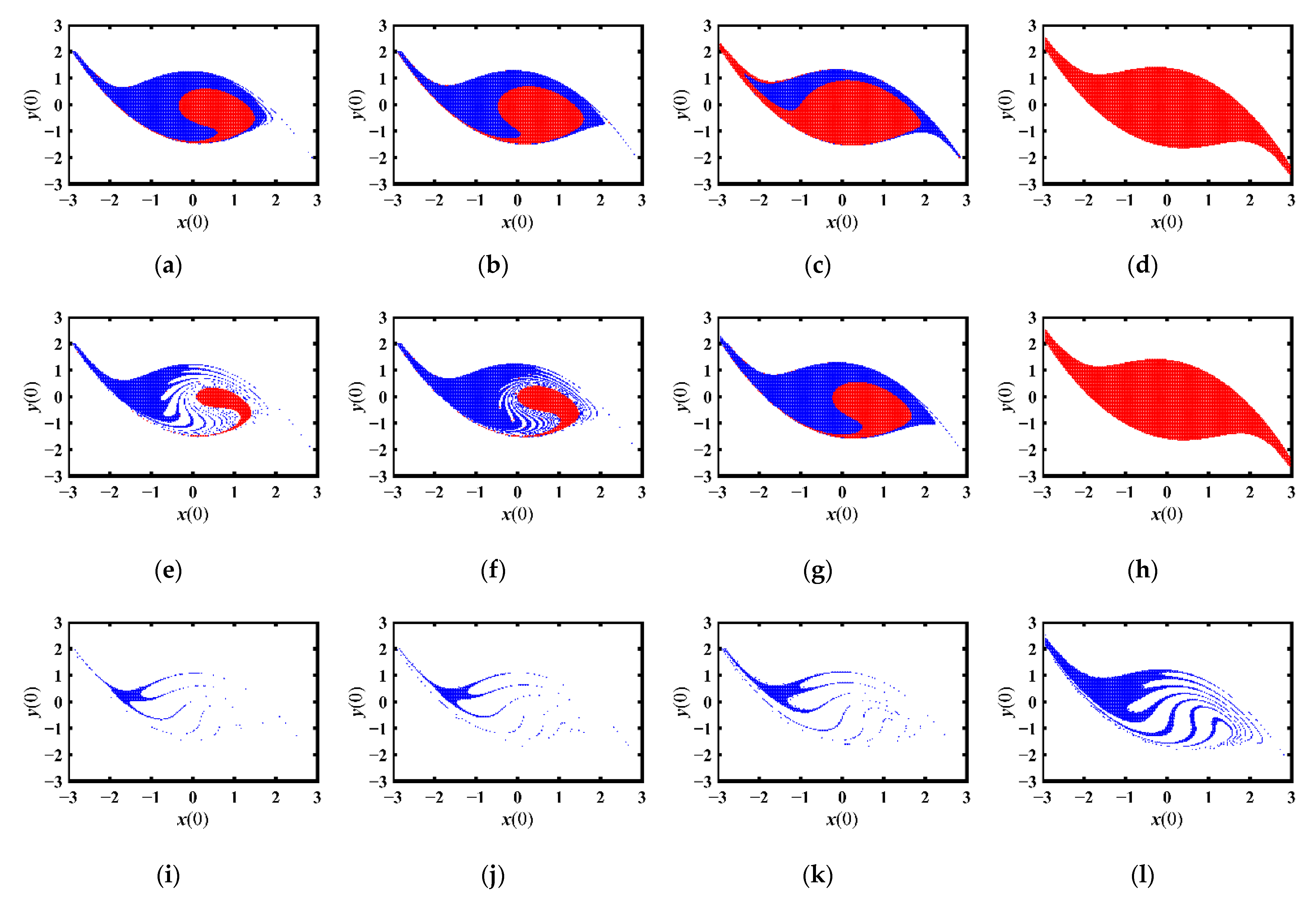
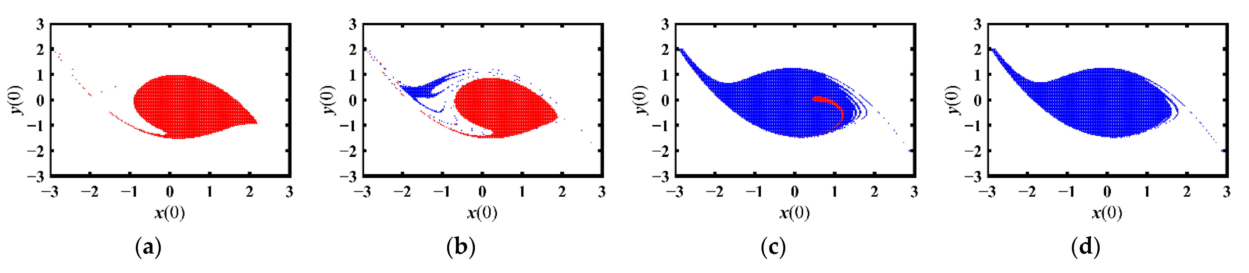
3.2. Initial-Sensitive Excessive Motion

Excessive motion of the system (6) can be understood as an escape or unbounded solution [21], for instance, a relative rotating angle in system (6) more than the material of the structure can bear. This may be induced by the variation of the system parameters or the initial conditions of the system. In the latter case, excessive motion coexists with bounded, meaning that a tiny disturbance of initial conditions leads to a change of dynamical behavior, such as from bounded vibration to unbounded. This is a typical initial-sensitive phenomenon, initial-sensitive excessive motion, indicating the loss of global integrity of dynamic systems [3,8]. Since it is often due to global bifurcation [15,21], we apply the Melnikov method [23] to detect the conditions for it. Substituting the heteroclinic orbits (9) into the Melnikov function yields
M ±   ( t 0 ) = + ( μ y ( T ) g y 3 ( T ) + f cos ( ω ( T + t 0 ) ) ) y ( T ) d T = 2 2 μ 3 b 8 2 g 35 b 2 + 2 b π ω f csch ( 2 π ω 2 ) cos ( ω t 0 ) .
For
2 b π ω f csch ( 2 π ω 2 ) 2 2 μ 3 b + 8 2 g 35 b 2 ,
Namely,
f f 0 = 2 ( 35 μ b + 12 g ) sinh ( π ω 2 ) 105 π ω b 3 2 ,
there will be a value of t 0 satisfying M ±   ( t 0 ) = 0 and M ±   ( t 0 ) 0 , meaning that the roots of Equation M ±   ( t 0 ) = 0 are simple, enabling the existence of the transverse heteroclinic orbits, and the system (6) may undergo initial-sensitive motion. According to Equation (26), f0 is the amplitude threshold of heteroclinic bifurcation. For parameter values given by Equation (23), the critical value for heteroclinic bifurcation is f0 = 0.09. In contrast, it follows from Inequation (25) that the threshold of the excitation frequency ω for heteroclinic bifurcation cannot be expressed as an explicit or monotonic increasing function of other parameters. For example, for f = 0.13 and the values of parameters in Equation (3), it can be calculated from Equation (25) that for ω < 1.22, heteroclinic bifurcation will occur in the system (6).
In order to verify the criterion obtained in this subsection, numerical simulations are carried out by fixing parameter values as in Equation (23). The 4th Runge-Kutta approach and the point-mapping method [24] are employed to describe the phenomenon’s initial-sensitive excessive motion. First, some terms such as basin of attraction and safe basin are introduced briefly. A basin of attraction is defined as the set of initial conditions that can lead to the same attractor [25]. If the boundary of basin of attraction of an attractor is fractal and mixed with another, jump among multiple attractors may occur [25]. Safe basin is defined as the union of basins of attraction for all bounded attractors [26]. Fractal of the safe basin of the system (6) induces the occurrence of initial-sensitive excessive motion. In this paper, the basin of attraction is drawn in the sufficiently large space region defined as −3.0 ≤ x(0) ≤ 3.0, −3.0 ≤ y(0) ≤ 3.0 by generating a 600 × 600 array of starting conditions, for each of these starting points. The escaping set for infinite time is approximated with good accuracy by a study with 1000 excited circles. The time step is taken as 0.01. The white region represents the numerical approximation to the basins of attraction of excessive motion. The red and blue regions are the basins of attraction for attractors from lower and higher stable periodic brunches of Figure 3, respectively. Thus, the union of the red region and the blue is the so-called safe basin.
The evolution of basins of attraction with the frequency ω for f = 0.13 and with the amplitude f for ω = 0.80 can be observed in Figure 4 and Figure 5. In Figure 4, each the safe basins, i.e., the union of red region and blue, is fractal-eroded when ω ranges from 0.62 to 0.87 satisfying ω < 1.22 i.e., the condition of heteroclinic bifurcation, which shows the occurrence of initial-sensitive excessive motion, in agreement with the analytical prediction. In Figure 4a, there is only a red region, meaning that there is only one periodic attractor from the lower stable branch. When ω = 0.69 (see Figure 4b), the red region and the blue one coexists, showing bistability. Specifically, on the left side of the origin, the red region is fractal and mixed with the white region and the blue, indicating that both jump and initial-sensitive excessive motion may occur there. As ω increases to 0.81 (see Figure 4c), most areas of the red region will be eroded by the blue one, showing that most of the safe initial conditions lead to the higher-amplitude attractor. For ω = 0.87 (see Figure 4d), the red region disappears, and there is only the blue, which means that the response shifts from the lower-amplitude branch to the higher-amplitude, in agreement with the theoretical results of Figure 3a.
In Figure 5, the safe basin (the union of red and blue regions) is steadily eroded by the white region with the increase of the amplitude f, implying that initial-sensitive excessive motion can be induced by the increase of f. In Figure 5a,b, the boundary of safe basins is smooth. When f is more than 0.09, i.e., the critical threshold solved from Equation (26), the boundary of safe basin will become fractal (see Figure 5c,d). In Figure 5a–c, the red region and the blue one are mixed, indicating bi-stability as well as jump. Note that for f = 0.12, the red and blue regions are evenly mixed in the neighborhood of the origin (see Figure 5c). For f = 0.20, only the basin of attraction of the attractors in the higher stable branch of Figure 3b exists, which is seriously eroded by the white region, showing that the excessive motion is easy to trigger.

4. Time-Delay Feedback to Control Complex Dynamics

In this section, two types of linear delay feedback controllers, i.e., delayed position feedback and delayed velocity feedback, are applied to the system (1), and their effect on suppressing the phenomena jump and initial-sensitive excessive motion is discussed. The corresponding control diagram is shown in Figure 6 where Q is the coefficient of the gain, and τ time delay. P ( θ 1 , θ 2 , θ ˙ 1 , θ ˙ 2 , θ 1 τ , θ 2 τ , θ ˙ 1 τ , θ ˙ 2 τ ) represents delayed relative-angle feedback ( θ 1 ( t τ ) θ 2 ( t τ ) ) ( θ 1 ( t ) θ 2 ( t ) ) or delayed relative-angular-velocity feedback ( θ ˙ 1 ( t τ ) θ ˙ 2 ( t τ ) ) ( θ ˙ 1 ( t ) θ ˙ 2 ( t ) ) , which is an active control transferring the motion state/velocity of the dynamical system [27]. The corresponding governing equation is
J 1 θ ¨ 1 + c 12 ( θ ˙ 1 θ ˙ 2 ) + K 1 ( θ 1 θ 2 ) + K 3 ( θ 1 θ 2 ) 3 + f 12 Q P ( θ 1 , θ 2 , θ ˙ 1 , θ ˙ 2 , θ 1 τ , θ 2 τ , θ ˙ 1 τ , θ ˙ 2 τ ) = T e 1 , J 2 θ ¨ 2 + c 12 ( θ ˙ 1 θ ˙ 2 ) + K 1 ( θ 1 θ 2 ) + K 3 ( θ 1 θ 2 ) 3 + f 12 + Q P ( θ 1 , θ 2 , θ ˙ 1 , θ ˙ 2 , θ 1 τ , θ 2 τ , θ ˙ 1 τ , θ ˙ 2 τ ) = T e 2 .
Letting
G p = J 1 + J 2 J 1 J 2 Q , G v = J 1 + J 2 J 1 J 2 Q ω 0 , τ ˜ = ω 0 τ ,
and based on Equations (2)–(6), we obtain the relative rotation system under delayed position feedback control, i.e.,
d x d T = y , d y d T = μ y x + b x 3 g y 3 + f cos ( ω T ) + G p ( x ( T τ ˜ ) x ( T ) ) ,
and the following delayed-velocity-feedback controlled system
y = d x d T , d y d T = μ y x + b x 3 g y 3 + f cos ( ω T ) + G v ( y ( T τ ˜ ) y ) .
In the delayed-feedback-controlled systems (29) and (30), G p , G v and τ ˜ are independent parameters. For G = 0 or τ ˜ = 0 , the feedback terms in Equations (29) and (30) become 0, and the delayed systems (29) and (30) become the uncontrolled non-dimensional system (6). In this paper, considering the engineering application, we do not consider the periodic characteristics of τ ˜ but restrict that 0 τ ˜ 2 π . Since there is no signal returned to the controlled systems (29) and (30) before T = 0 , it is supposed that the initial states of the delayed system when τ ˜ T < 0 satisfy x ( T ) = y ( T ) = 0 . Then, safe basins of the delayed-feedback controlled systems can also be projected into the initial-state plane x ( 0 ) y ( 0 ) , similar to the uncontrolled system (6).

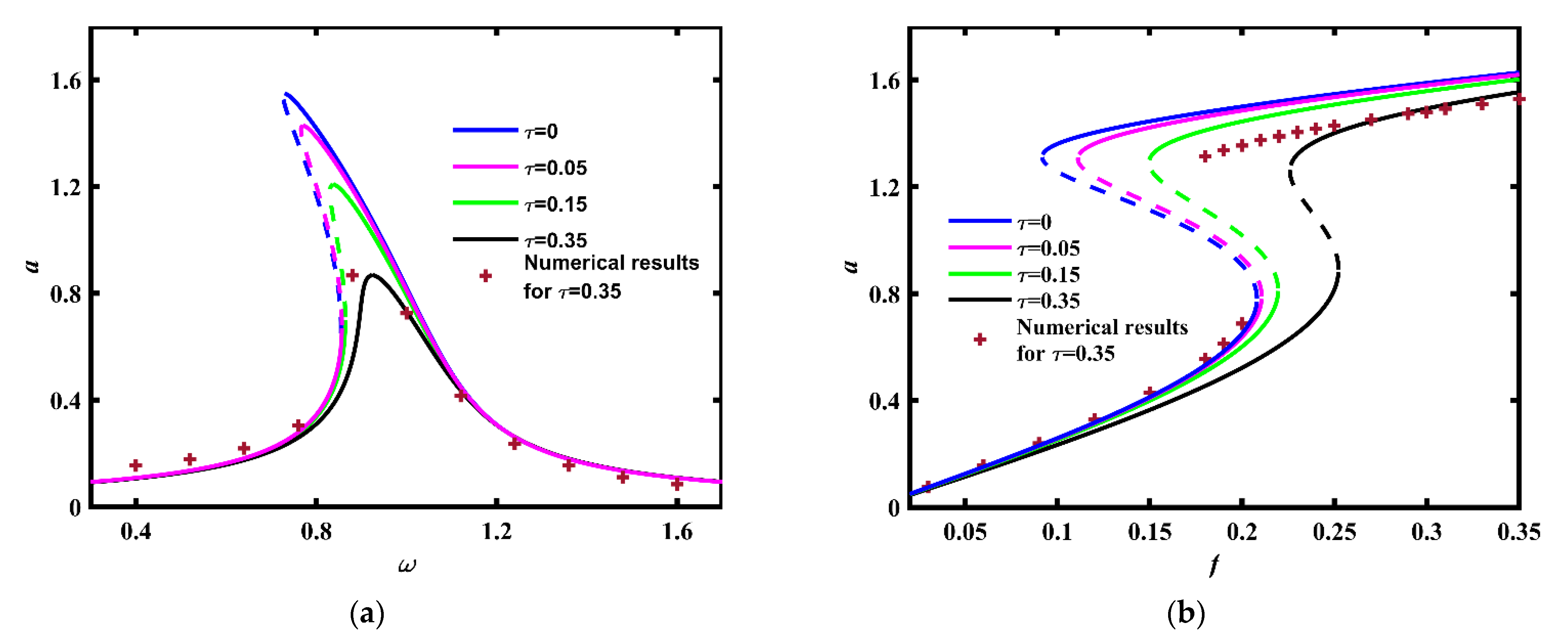
4.1. Delayed Position Feedback Control

4.1.1. Primary Resonant Response and Stability of Solutions

As discussed in Section 3.1, the Method of Multiple Scales is applied to obtain the periodic response of the delayed system. Rescaling the gain as G p = ε G ˜ p , and following the similar procedure as in Section 3.1, one can finally obtain the slow flow equation:
d a d T = μ a 2 3 g a 3 8 + f sin ψ 2 a G p sin τ ˜ 2 , a d ψ d T = ( ω 1 ) a + 3 b a 3 8 + f cos ψ 2 a G p ( 1 cos τ ˜ ) 2 .
One can get the amplitude and the phases of the response by equating the right sides of Equation (31) to zero, i.e.,
μ a + 3 g a 3 4 + a G p sin τ ˜ = f sin ψ , 2 ( ω 1 ) a 3 b a 3 4 + a G p ( 1 cos τ ˜ ) = f cos ψ .
Accordingly, the approximate periodic solution can be expressed as x 0 = a cos ( ω T ψ ) . Its amplitude a can be solved from the following equation
( μ + G p sin τ ˜ + 3 g a 2 4 ) 2 a 2 + ( 2 ω 2 + 3 4 b a 2 + G p cos τ ˜ G p ) 2 a 2 = f 2 .
The stability of the solutions, thus obtained, can be ascertained by computing the eigenvalues from the corresponding characteristic equation:
λ 2 + λ ( μ + G p sin τ ˜ + 3 g a 2 2 ) + 27 ( g 2 + b 2 ) a 4 64 + ( μ + G p sin τ ˜ ) 2 4 + ( ω 1 + G p cos τ ˜ G p 2 ) 2 + 3 a 2 4 ( g G p sin τ ˜ + b G p cos τ ˜ + b ( 2 ω 2 G p ) + g μ ) = 0 .
Assuming λ = i v in Equation (34) and separating the real and imaginary parts, we have
v ( μ + G p sin τ ˜ + 3 g a 2 2 ) = 0
and
v 2 + 27 ( g 2 + b 2 ) a 4 64 + ( μ + G p sin τ ˜ ) 2 4 + ( ω 1 + G p cos τ ˜ G p 2 ) 2 + 3 a 2 4 ( g G p sin τ ˜ + b G p cos τ ˜ + b ( 2 ω 2 G p ) + g μ ) = 0 .
As we know, when the delay is small, the delayed feedback can be expanded in a Taylor series so that the controlled system (29) will become
d x d T = y , d y d T = ( μ + G p τ ˜ ) y x + b x 3 g y 3 + f cos ( ω T ) .
For G p > 0 , it is much like increasing the damping of the system (6), thus reducing the periodic vibration [20,27]. Letting G p > 0 , one has μ + G p sin τ ˜ + 3 g a 2 2 > 0 for 0 τ ˜ π . Thus, v = 0 in Equation (35); if
27 ( g 2 + b 2 ) a 4 64 + 3 a 2 4 ( g G p sin τ ˜ + b G p cos τ ˜ + b ( 2 ω 2 G p ) + g μ ) + ( ω 1 + G p cos τ ˜ G p 2 ) 2 + ( μ + G p sin τ ˜ ) 2 4 = 0 ,
saddle-node bifurcation will occur in the periodic branch. For G p > 0 , when τ ˜ is long enough to satisfy
( g G p sin τ ˜ + b G p cos τ ˜ + b ( 2 ω 2 G p ) + g μ ) 2 3 ( g 2 + b 2 ) ( ( ω 1 G p 2 + G p cos τ ˜ 2 ) 2 + ( μ + G p sin τ ˜ ) 2 4 ) < 0 ,
there will be no positive roots for Equation (38), meaning under a positive gain, the delayed position feedback can be used to reduce saddle-node bifurcation and thus bi-stability. For example, given Gp = 0.3 and ω = 0.8, one can calculate from Equation (39) that there is no saddle-node bifurcation for τ ˜ > 0.63 . In contrast, it is hard to express the range of τ ˜ for saddle-node bifurcation as a function of f. Fixing the value of f and combining Equations (33), (38) and (39), one can obtain the condition for τ ˜ to reduce saddle-node bifurcation. For instance, given f = 0.13, one can calculate that the condition of τ ˜ to reduce saddle-node bifurcation is τ ˜ > 0.27.
Based on the above theoretical analysis, the results are verified by numerical simulation as shown in Figure 7. Figure 7a shows the frequency-response for f = 0.13, Gp = 0.3 and different values of time delay satisfying τ ˜ < < π . Obviously, in Figure 7a, the amplitude of the response reduces with the increase in time delay. Note that for τ ˜ = 0.35 (longer than the theoretical values 0.27), there is no saddle-node bifurcation on the periodic branches, showing that bi-stability and jump will not occur. It can be seen from Figure 7a that the increase of time delay in the position feedback can reduce saddle-node bifurcation, and thus bi-stability and jump. This can also be verified by the evolution of basins of attraction with the increase of time delay (see Figure 8). It follows from Figure 8 that as τ ˜ increases, the basin of attraction of the higher-amplitude periodic attractor (the blue region) will be eroded by the basin of attraction of the lower-amplitude one (see the red region). Meanwhile, the safe basin (red and bule regions) becomes smooth. For ω = 0.80, one can see from Figure 7b that even though the saddle-node bifurcation still exists, increase of time delay can help to reduce the range of f where bistable attractors coexist. The corresponding sequences of basin of attraction with the increase of f and τ ˜ will be discussed in detail in the next subsection.

4.1.2. Heteroclinic Bifurcation

To employ the Melnikov method to analyze the critical condition for heteroclinic bifurcation in a delayed-feedback-controlled system, it is necessary to consider the delayed position feedback as a perturbed term, namely, the values of the delay and the gain should satisfy that the stability of the equilibrium of the uncontrolled linear system cannot be changed by the delayed feedback. Since the equilibrium S1(0,0) is stable for μ > 0, the delay should not exceed the first value of the stability switch of the following linear delayed system
d 2 x d T 2 + μ d x d T + x = G p ( x ( T τ ˜ ) x ( T ) ) .
Its characteristic equation is given by
λ 2 + μ λ + 1 + G p G p e λ τ ˜ = 0 .
Substituting λ = i v into (41) and separating the imaginary and real parts yields
Ω p 2 + 1 + G p G p cos ( Ω p τ ˜ ) = 0 , μ Ω p + G p sin ( Ω p τ ˜ ) = 0 .
By eliminating the trigonometric functions, Equation (42) becomes
Ω p 4 ( 2 + 2 G p μ 2 ) Ω p 2 + 1 + 2 G p = 0 .
For
G p > max { μ 2 2 1 , μ 2 2 + μ } ,
there are two different positive solutions of Equation (43) expressed as Ω p 1 and Ω p 2 ( Ω p 1 > Ω p 2 > 0 ); the critical value of the delay for stability switch of S1(0,0) is
τ 0 = 1 Ω p 1 ( 2 π arccos ( 1 + 1 Ω p 1 2 G p ) ) .
For τ ˜ < τ 0 , the delay position feedback can be regarded as a disturbed term.
Substituting the heteroclinic orbits (9) into the Melnikov function of the system (29) yields
M ±   ( t 0 ) = 2 2 μ 3 b 8 2 g 35 b 2 + 2 b π ω f csch ( π ω 2 ) cos ( ω t 0 ) G p b l 1 ( τ ˜ ) ,
where l 1 ( τ ˜ ) = csch 2 ( 2 2 τ ˜ ) ( sinh ( 2 τ ˜ ) 2 τ ˜ ) > 0 . The critical condition for heteroclinic bifurcation can be expressed as
f > f P ( τ ˜ ) = f 0 + G p sech ( π ω 2 ) l 1 ( τ ˜ ) π 2 b ω ,
Accordingly, for G p > 0, the threshold of heteroclinic bifurcation f P ( τ ˜ ) will increase with time delay and be higher than f0. Fixing µ = 0.02 and Gp = 0.3, it can be calculated that τ0 = 2.55.
Figure 9 shows the variation of f P ( τ ˜ ) with the increase of time delay τ ˜ ( τ ˜ << τ0). Then the numerical values of f P ( τ ˜ ) are obtained at which the boundary of the safe basin begin to be unsmooth. Each numerical critical value of f P ( τ ˜ ) is kept at two decimal places. We make sure that if f is less than the numerical results f P ( τ ˜ ) , the boundary of safe basin will be smooth. In Figure 9, the numerical results for the critical values of f are in agreement with the analytical values, demonstrating that the threshold of the amplitude f for heteroclinic bifurcation will increase monotonically with the delay for G p > 0 and τ ˜ < τ 0 .
Figure 10 depicts the evolution of the safe basin of the controlled system (29) with the delay τ ˜ . In Figure 10a,e,i for τ ˜ = 0 , safe basins as well as basins of attraction can be considered as those of the uncontrolled system (6), illustrating that as the amplitude f increases, safe basin will be eroded. Specifically, in Figure 10e for f = 0.30, only the basin of attraction of the higher-amplitude attractor is left, which is seriously eroded by the white region, showing the high possibility of excessive motion. For Gp = 0.3 and τ ˜ = 0.11, the safe basin is obviously expanded. Besides, comparing Figure 10a–d, one can observe that as τ ˜ increases, the safe basin changes from the union of red region and blue to the red region itself, meaning that jump and initial-sensitive excessive motion are reduced by the basin expansion of the lower-amplitude attractor. In Figure 10e–h, one can also draw this conclusion. Note that Figure 10e,f, three color regions are mixed in the neighborhood of the origin, which indicates the high probability of jump and initial-sensitive excessive motion. As τ ˜ increases, they can be controlled. For f = 0.30 (see Figure 10i–l), even though the safe basin is still fractal, its area becomes much larger with the increase of τ ˜ . This shows that the possibility of excessive motion is reduced. It follows from Figure 9 that the delayed position feedback can suppress the erosion of the safe basin effectively when Gp is positive.

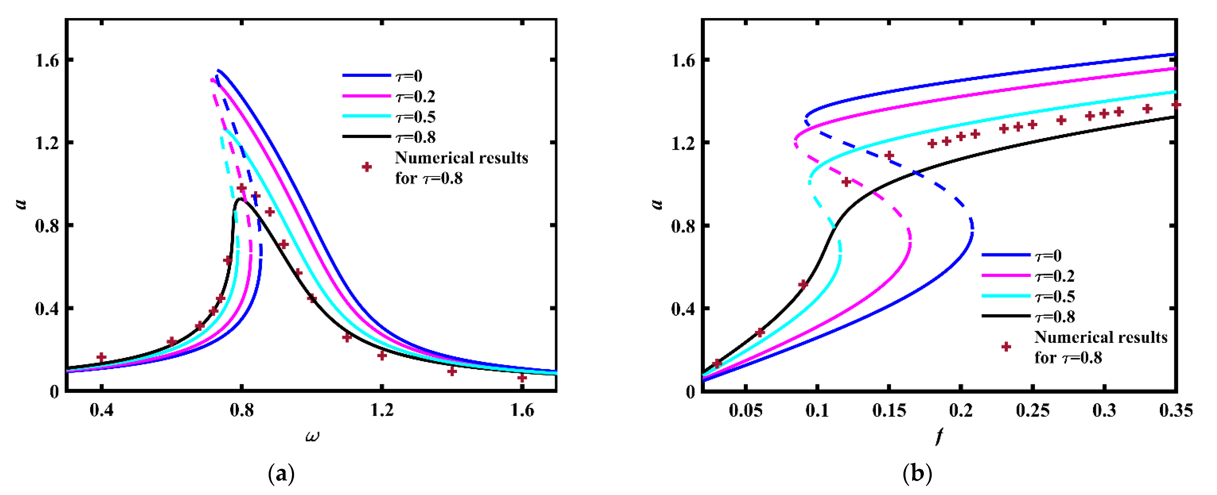
4.2. Delayed Velocity Feedback

4.2.1. Primary Resonant Response and Stability of Solutions

As in Section 4.1.1, by applying the Method of Multiple Scales, one can get the slow flow equation of the delayed-velocity-feedback controlled system (30) as below:
d a d T = μ 2 a 3 g a 3 8 + f sin ψ 2 G v ( 1 cos τ ˜ ) 2 a , a d ψ d T = a ( ω 1 ) + 3 b a 3 8 + f cos ψ 2 + G v sin τ ˜ 2 a .
The amplitude and phases of the system can be obtained via letting the right side of Equation (48) be zero, given by
f sin ψ = μ a + 3 g 4 a 3 + G v ( 1 cos τ ˜ ) a , f cos ψ = ( 2 2 ω 3 b 4 a 2 G v sin τ ˜ ) a .
Thus, the amplitude of the approximated periodic solution x 0 = a cos ( ω T ψ ) can be solved from the following equation:
( μ + 3 g 4 a 2 + G v ( 1 cos τ ˜ ) ) 2 a 2 + ( 2 2 ω 3 b 4 a 2 G v sin τ ˜ ) 2 a 2 = f 2 .
According to its characteristic equation, the stability switch will occur if there exists a real number v ˜ satisfying
v ( μ + G v ( 1 cos τ ˜ ) + 3 g a 2 2 ) = 0 , v 2 + ( μ + G v ( 1 cos τ ˜ ) ) 2 4 + ( 2 2 ω G v sin τ ˜ ) 2 4 + μ 2 G v ( 1 cos τ ˜ ) + 3 a 2 4 ( μ g + b ( 2 ω 2 + G v sin τ ˜ ) ) + 27 ( g 2 + b 2 ) a 4 64 = 0 .
For G v > 0 , in Equation (51), one has μ + 3 g 2 a 2 + G v ( 1 cos τ ˜ ) > 0 , v ˜ = 0, and
( μ + G v ( 1 cos τ ˜ ) ) 2 4 + ( 2 2 ω G v sin τ ˜ ) 2 4 + μ 2 G v ( 1 cos τ ˜ ) + 3 a 2 4 ( μ g + b ( 2 ω 2 + G v sin τ ˜ ) ) + 27 ( g 2 + b 2 ) a 4 64 = 0 ,
implying that saddle-node bifurcation will occur in the delayed-velocity-feedback controlled system. For G v > 0 , when τ ˜ is long enough to satisfy
4 ( μ g + b ( 2 ω 2 ) + b G v sin τ ˜ ) 2 3 ( g 2 + b 2 ) ( ( μ + G v ) 2 + 2 μ G v + G v 2 + 4 ( 1 ω ) 2 2 G v ( 2 μ + G v ) cos τ ˜ + 4 ( ω 1 ) G v sin τ ˜ ) < 0 ,
there will be no positive roots for Equation (52), meaning no saddle-node bifurcation or bi-stability. For example, given Gv = 0.3 and ω = 0.8, one can calculate from Equation (53) that saddle-node bifurcation will disappear for τ ˜ > 0.68 . Similarly to Section 4.1.1, although delayed velocity feedback can be used to reduce the occurrence of saddle-node bifurcation, it is hard to express the range of τ ˜ for SN bifurcation as a function of f. Fixing the value of f and combining Equations (50), (52) and (53), one can obtain the condition for τ ˜ to reduce saddle-node bifurcation. For instance, given f = 0.13, one can calculate that the condition of τ ˜ to reduce saddle-node bifurcation is τ ˜ > 0.77.
The similar as in Section 4.1.1, for Gv = 0.3 and different values of time delay in the velocity feedback, Figure 11 shows the variation of the response amplitude with the excitation. It follows from the theoretical and numerical results depicted in Figure 11 that, even though the response amplitude is not necessary to be suppressed with the increase of time delay, the velocity feedback can reduce saddle-node bifurcation, and thus bi-stability and jump. The controlling effect of velocity feedback on jump can also be verified by the evolution of basins of attraction with the increase of time delay for f = 0.13, ω = 0.78 (see Figure 12). To be different from the case of the delayed position feedback, as the delay increases, the basin of attraction of the higher-amplitude attractor is expanded, whose boundary becomes smoother and smoother. Finally, it becomes the only bounded attractor (see Figure 12d). For ω = 0.80, if can be concluded from Figure 11b that the delayed velocity feedback can suppress bi-stability. For the fixed value of ω, sequences of the basin of attraction with the increase of f and τ ˜ will be discussed in detail in the next subsection.

4.2.2. Heteroclinic Bifurcation under Delayed Velocity Feedback

As in Section 4.1.2, to apply the Melnikov method in the delayed-velocity-feedback controlled system (30), we also need to treat the delayed feedback as a perturbed term of this system. To this end, the delay τ ˜ should not exceed the first value of stability switch of S1(0,0) in the linear delayed system whose characteristic equation can expressed as
λ 2 + μ λ + 1 + G v λ G v λ e λ τ ˜ = 0
.
The first value of time delay for stability switch of S1(0,0) will occur when λ = ± Ω v i . Substituting it into Equation (54) and separating the imaginary and the real parts of Equation (54) yields
Ω v 2 + 1 = G v Ω v sin ( Ω v τ ˜ ) , μ Ω v = G v Ω v ( cos ( Ω v τ ˜ ) 1 ) .
By eliminating the trigonometric functions, the equation above becomes
( Ω v 2 1 ) 2 + ( μ 2 + 2 μ G v ) Ω v 2 = 0 .
Since μ > 0 , for G v > 0 , there will be no real roots of Equation (56), meaning that the stability of the origin will not be changed. Then the delay velocity feedback of the delayed system (30) can be regarded as a disturbed term. The Melnikov function of the controlled system (30) can be expressed as
M ±   ( t 0 ) = + ( μ y ( T ) g y 3 ( T ) + f cos ( ω ( T + t 0 ) ) G v y ( T ) + G v y ( T τ ˜ ) ) y ( T ) d T = 2 2 μ 3 b 8 2 g 35 b 2 + 2 b π ω f csch ( 2 π ω 2 ) cos ( ω t 0 ) 2 G v b l 2 ,
where l 2 ( τ ˜ ) = csch 2 ( 2 τ ˜ 2 ) ( 2 τ ˜ coth ( 2 2 τ ˜ ) ) > 0 . Accordingly, for
f > f V ( τ ˜ ) = f 0 + 2 b G v b π ω sinh ( 2 π ω 2 ) l 2 ( τ ˜ ) ,
And heteroclinic bifurcation may occur. In Equation (58), for G v > 0, the threshold of heteroclinic bifurcation f V ( τ ˜ ) increases monopoly with the delay τ ˜ . Given G v = 0.3, the variation of f V ( τ ˜ ) with the increase of τ ˜ is presented in Figure 13. Numerical and analytical results both illustrate that, for G v > 0, the delayed velocity feedback can be used to increase the threshold of the amplitude f for heteroclinic bifurcation, thus being effective in reducing the probability of initial-sensitive excessive motion.
Figure 14 shows the evolution of the safe basin of the controlled system (30) with the increase of f and τ ˜ . For τ ˜ = 0, Figure 14a,e,i are the same as Figure 10a,e,i, depicting the safe basin of the uncontrolled system (6). Under a positive gain Gv = 0.3, when τ ˜ increases, the area of safe basin of the delayed-velocity-feedback-controlled system will expand obviously. To be different from the results of Section 4.1.2, for f = 0.11 and 0.15 where the two periodic attractors coexisting in the uncontrolled system, as τ ˜ increases, the basin of attraction of the higher-amplitude attractor is expanded and finally becomes the safe basin (see the blue regions in Figure 14a–h). This illustrates that, although the delayed velocity feedback does not necessary reduce the response amplitude, it reduces jump and excessive motion.

5. Discussion

In this paper, a typical relative rotation system is considered, and the phenomena of jump and initial-sensitive excessive motion as well as their suppression via delayed feedback is investigated. The Method of Multiple Scales and the Melnikov method are applied to analyze the conditions for bi-stability and initial-sensitive excessive motion, respectively. By introducing the basins of attraction and safe basin to describe the extent of jump and initial-sensitive excessive motion, respectively, the point mapping approach is employed to present the numerical results which matches the theoretical approach, verifying the validity of the analysis. Some significant results are presented as follows.
(1)
The variation of excitation may induce the coexistence of bistable periodic attractors, which can be ascribed to saddle-node bifurcation.
(2)
The increase of the excitation amplitude may cause initial-sensitive excessive motion, which can be due to heteroclinic bifurcation.
(3)
Under positive coefficients of the feedback gain, the delayed position feedback and the delayed velocity feedback can reduce saddle-node bifurcation and heteroclinic bifurcation so as to suppress jump and initial-sensitive excessive motion. Comparatively, the former can also reduce the amplitude of the response, while the latter may not; the former works well if time delay does not exceed the first stability switch of the trivial equilibrium, while the latter does not have that restriction.
This work presents a detailed analysis of jump and initial-sensitive excessive motion of a typically relative rotation system, which may be beneficial for the performance improvement of rotors and main bearings. The relevant experimental investigations will be included in our future work.

Author Contributions

Conceptualization, H.S.; formal analysis, H.S.; funding acquisition, H.S.; Investigation, Z.C.; methodology, H.S.; project administration, H.S.; software, Z.C.; supervision, H.S.; validation, H.S.; visualization, Z.C.; writing—original draft, Z.C. and H.S.; writing—review & editing, H.S. All authors have read and agreed to the published version of the manuscript.

Funding

This research was funded by the National Natural Science Foundation of China, grant number 11472176.

Institutional Review Board Statement

Not applicable.

Informed Consent Statement

Not applicable.

Data Availability Statement

Not applicable.

Conflicts of Interest

The authors declare no conflict of interest.

References

  1. Liang, Y.; Li, N. Optimal vibration control for nonlinear systems of tracked vehicle half-car suspensions. Int. J. Control. Autom. Syst. 2017, 15, 1675–1683. [Google Scholar] [CrossRef]
  2. Renson, L.; Noël, J.P. Complex dynamics of a nonlinear aerospace structure: Numerical continuation and normal modes. Nonlinear Dyn. 2015, 79, 1293–1309. [Google Scholar] [CrossRef] [Green Version]
  3. Shi, J.; Gou, X. Bifurcation and Erosion of Safe Basin for a Spur Gear System. Int. J. Bifurc. Chaos 2018, 28, 1830048. [Google Scholar] [CrossRef]
  4. Li, J.; Wu, H. Bifurcation, chaos, and their control in a wheelset model. Math. Methods Appl. Sci. 2020, 43, 7152–7174. [Google Scholar] [CrossRef]
  5. Luo, Z.; Wang, J. Research on vibration performance of the nonlinear combined support-flexible rotor system. Nonlinear Dyn. 2019, 98, 113–128. [Google Scholar] [CrossRef]
  6. Li, Y.; Luo, Z. Dynamic modeling and stability analysis of a rotor-bearing system with bolted-disk joint. Mech. Syst. Signal Process. 2021, 158, 107778. [Google Scholar] [CrossRef]
  7. Shi, P.; Liu, B. Chaotic motion of some relative rotation nonlinear dynamic system. Acta Phys. Sin. 2008, 57, 1321–1328. [Google Scholar]
  8. Li, Z.; Gou, X. Erosion and bifurcation of safety-attraction basin for multi-state meshing gear transmission system under tooth safety condition. J. Vbration Shock 2021, 40, 63–74. [Google Scholar]
  9. Wang, K.; Guan, X. Precise periodic solutions and uniqueness of periodic solutions of some relative rotation nonlinear dynamic system. Acta Phy. Sin. 2010, 59, 3648–3653. [Google Scholar] [CrossRef]
  10. Xiao, L.; Xuan, C. The periodic solution problem of a relative rotation nonlinear dynamic system with time-varying stiffness. Acta Phy. Sin. 2013, 62, 21–25. [Google Scholar]
  11. Li, X.; Yan, J. The periodic solution problem of a relative rotation nonlinear system with nonlinear elastic force and generalized damping force. Acta Phy. Sin. 2014, 63, 36–41. [Google Scholar]
  12. Shi, P.; Han, D. Chaos and chaotic control in a relative rotation nonlinear dynamical system under parametric excitation. Chin. Phys. B 2010, 19, 116–121. [Google Scholar]
  13. Verichev, N. Chaotic torsional vibration of imbalanced shaft driven by a limited power supply. J. Sound Vib. 2012, 331, 384–393. [Google Scholar] [CrossRef]
  14. Liu, B.; Zhao, H. Bifurcation and chaos of some relative rotation system with triple-well Mathieu-Duffing oscillator. Acta Phy. Sin. 2014, 63, 174502. [Google Scholar]
  15. Liu, S.; Tian, S. Chaos of a kind of nonlinear relative rotation system based on the effect of Coulomb friction. Acta Phy. Sin. 2015, 64, 247–254. [Google Scholar]
  16. Zhu, L.; Li, Z. Evolutionary mechanism of safety performance for spur gear pair based on meshing safety domain. Nonlinear Dyn. 2021, 104, 215–239. [Google Scholar] [CrossRef]
  17. Ju, J.; Wei, L. Dynamics and nonlinear feedback control for torsional vibration bifurcation in main transmission system of scraper conveyor direct-driven by high-power PMSM. Nonlinear Dyn. 2018, 93, 307–321. [Google Scholar] [CrossRef]
  18. Shang, H. Pull-in instability of a typical electrostatic MEMS resonator and its control by delayed feedback. Nonlinear Dyn. 2017, 90, 171–183. [Google Scholar] [CrossRef]
  19. Wang, Q.; Wu, H. The effect of fractional damping and time-delayed feedback on the stochastic resonance of asymmetric SD oscillator. Nonlinear Dyn. 2022, 107, 2099–2114. [Google Scholar] [CrossRef]
  20. Zhao, Y.; Li, C. The delayed feedback control to suppress the vibration in a torsional vibrating system. Acta Phy. Sin. 2011, 60, 417–425. [Google Scholar]
  21. Shang, H.; Han, Y. Suppression of chaos and basin erosion in a nonlinear relative rotation system by delayed position feedback. Acta Phy. Sin. 2014, 63, 88–95. [Google Scholar]
  22. Rezaei, M.; Khadem, E.S.; Friswell, I.M. Energy harvesting from the secondary resonances of a nonlinear piezoelectric beam under hard harmonic excitation. Meccanica 2020, 55, 1463–1479. [Google Scholar] [CrossRef]
  23. Siewe, S.M.; Hegazy, H.U. Homoclinic bifurcation and chaos control in MEMS resonators. Appl. Math. Model. 2011, 35, 5533–5552. [Google Scholar] [CrossRef]
  24. Danico, K.; Tanmoy, C.; Milan, C.; Sondipon, A.; Karličić, D.; Chatterjee, T.; Cajić, M.; Adhikari, S. Parametrically amplified Mathieu-Duffing nonlinear energy harvesters. J. Sound Vib. 2020, 488, 115677. [Google Scholar]
  25. Zhu, Y.; Shang, H. Multistability of the vibrating system of a micro resonator. Fractal Fract. 2022, 6, 141. [Google Scholar] [CrossRef]
  26. Rega, G.; Lenci, S. Dynamical integrity and control of nonlinear mechanical oscillators. J. Vib. Control 2008, 14, 159–179. [Google Scholar] [CrossRef] [Green Version]
  27. Liu, C.; Yan, Y.; Wang, W. Resonances and chaos of electrostatically actuated arch micro/nanoresonators with time delay velocity feedback. Chaos Solitons Fractals 2019, 10, 109512. [Google Scholar] [CrossRef]
Figure 1. Simplified diagram of a two-rotor torsional vibrating system.
Mathematics 10 02676 g001
Figure 2. Orbits of the unperturbed system (7) for b = 0.3.
Mathematics 10 02676 g002
Figure 3. Response curves of system (2). (a) Amplitude a vs. ω when f = 0.13; (b) Amplitude a vs. f when ω = 0.80.
Mathematics 10 02676 g003
Figure 4. Evolution of basins of attraction with the increase of ω for f = 0.13. (a) ω = 0.62; (b) ω = 0.69; (c) ω = 0.81; (d) ω = 0.87.
Mathematics 10 02676 g004
Figure 5. Evolution of basins of attraction with the increase of f for ω = 0.80. (a) f = 0.03; (b) f = 0.07; (c) f = 0.12; (d) f = 0.20.
Mathematics 10 02676 g005
Figure 6. Diagram of the relative rotating system under delayed feedback control.
Mathematics 10 02676 g006
Figure 7. Variation of the response amplitude of the system (29) with the excitation for Gp = 0.3. (a) f = 0.13; (b) ω = 0.80.
Mathematics 10 02676 g007
Figure 8. Evolution of basins of attraction with the increase of τ when f = 0.13 and ω = 0.78. (a) τ = 0; (b) τ = 0.05; (c) τ = 0.15; (d) τ = 0.35.
Mathematics 10 02676 g008
Figure 9. fP(τ) of the controlled system (29) versus time delay when Gp = 0.3 and ω = 0.80.
Mathematics 10 02676 g009
Figure 10. Sequences of safe basin of the system (29) with the increase of f and τ ˜ when Gp = 0.3. (a) f = 0.11, τ ˜ = 0; (b) f = 0.11, τ ˜ = 0.05; (c) f = 0.11, τ ˜ = 0.15; (d) f = 0.11, τ ˜ = 0.35; (e) f = 0.15, τ ˜ = 0; (f) f = 0.15, τ ˜ = 0.05; (g) f = 0.15, τ ˜ = 0.15; (h) f = 0.15, τ ˜ = 0.35; (i) f = 0.30, τ ˜ = 0; (j) f = 0.30, τ ˜ = 0.05; (k) f = 0.30, τ ˜ = 0.15; (l) f = 0.30, τ ˜ = 0.35.
Mathematics 10 02676 g010
Figure 11. Variation of the response amplitude of the system (30) with the excitation for Gv = 0.3. (a) f = 0.13; (b) ω = 0.80.
Mathematics 10 02676 g011
Figure 12. Evolution of basins of attraction with the increase of τ for f = 0.13 and ω = 0.78. (a) τ ˜ = 0; (b) τ ˜ = 0.2; (c) τ ˜ = 0.5; (d) τ ˜ = 0.8.
Mathematics 10 02676 g012
Figure 13. f V (τ) of the controlled system (30) versus time delay when Gv = 0.3.
Mathematics 10 02676 g013
Figure 14. Sequences of safe basin of the system (30) with the increase of f and τ ˜ when G v = 0.3. (a) f = 0.11, τ ˜ = 0; (b) f = 0.11, τ ˜ = 0.20; (c) f = 0.11, τ ˜ = 0.50; (d) f = 0.11, τ ˜ = 0.80; (e) f = 0.15, τ ˜ = 0; (f) f = 0.15, τ ˜ = 0.20; (g) f = 0.15, τ ˜ = 0.50; (h) f = 0.15, τ ˜ = 0.80; (i) f = 0.30, τ ˜ = 0; (j) f = 0.30, τ ˜ = 0.20; (k) f = 0.30, τ ˜ = 0.50; (l) f = 0.30, τ ˜ = 0.80.
Mathematics 10 02676 g014aMathematics 10 02676 g014b
Publisher’s Note: MDPI stays neutral with regard to jurisdictional claims in published maps and institutional affiliations.

