
Transmission Lines Impedance Fitting Using Analytical Impedance Equation and Frequency Response Analysis


Abstract
:1. Introduction
- Develop a fitting method for MTL impedance based on the analytical impedance equation. This will ensure that the proposed method behaves similarly to the transmission line impedance.
- Develop a fitting method for MTL impedance which is a function of transmission line length. This is to ensure that the proposed model will have an accurate representation of the transmission line impedance for different transmission line lengths.
- Develop a fitting method capable of fitting MTL impedance for a wide range of frequencies without modifying the model for higher frequencies.
2. Wave Characteristics on Finite Transmission Lines
- , attenuation constant, in Np/m.
- , phase constant, in rad/m.
- R, resistance per unit length, in /m.
- L, inductance per unit length, in H/m.
- G, conductance per unit length, in S/m.
- C, capacitance per unit length, in F/m.
- l, length of the transmission line, in m.
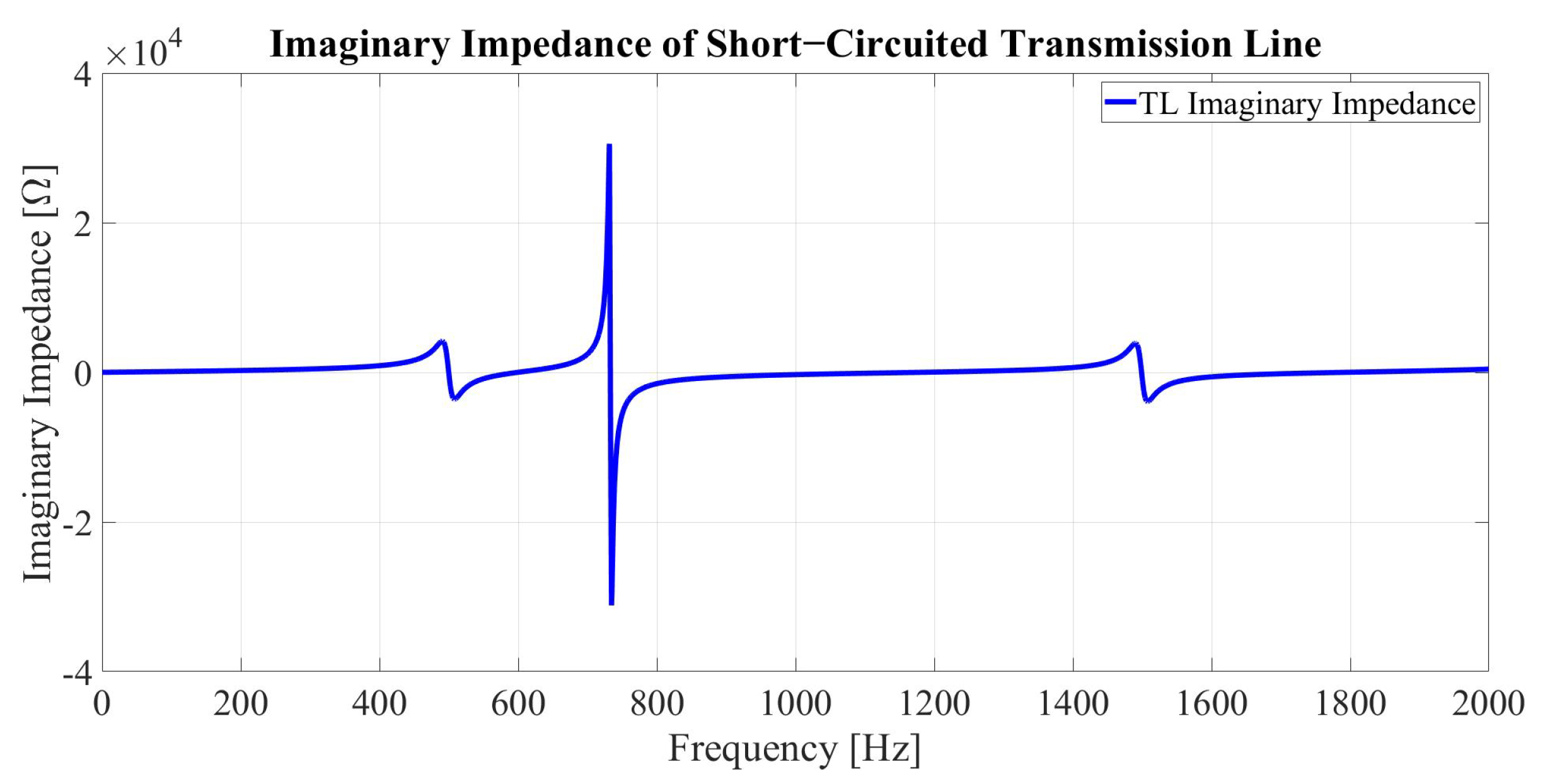
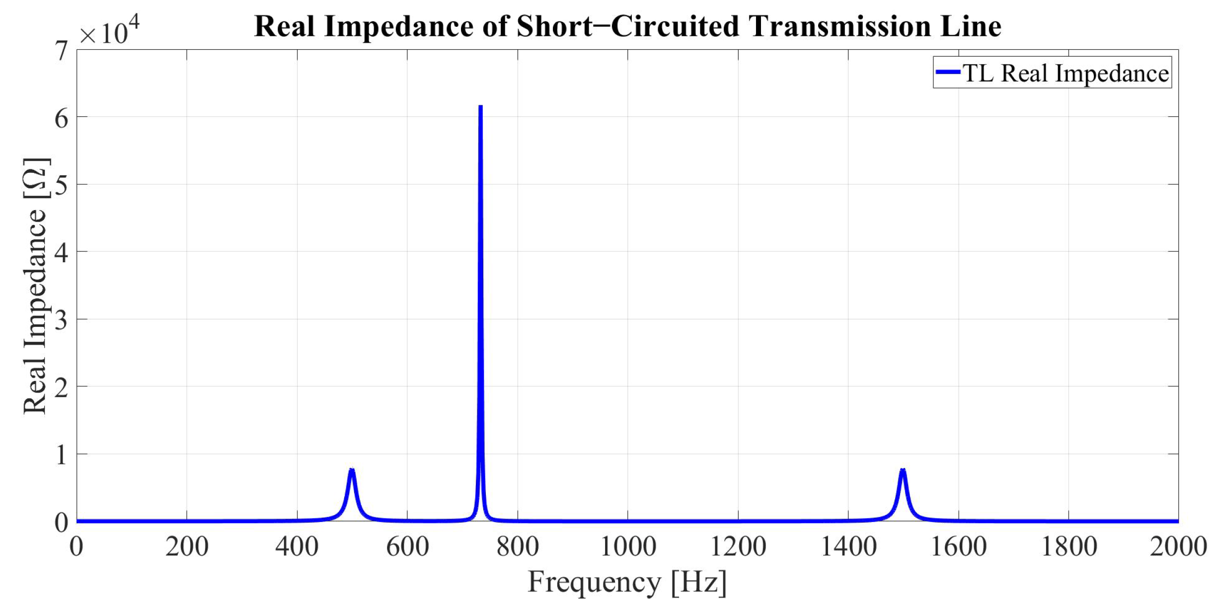
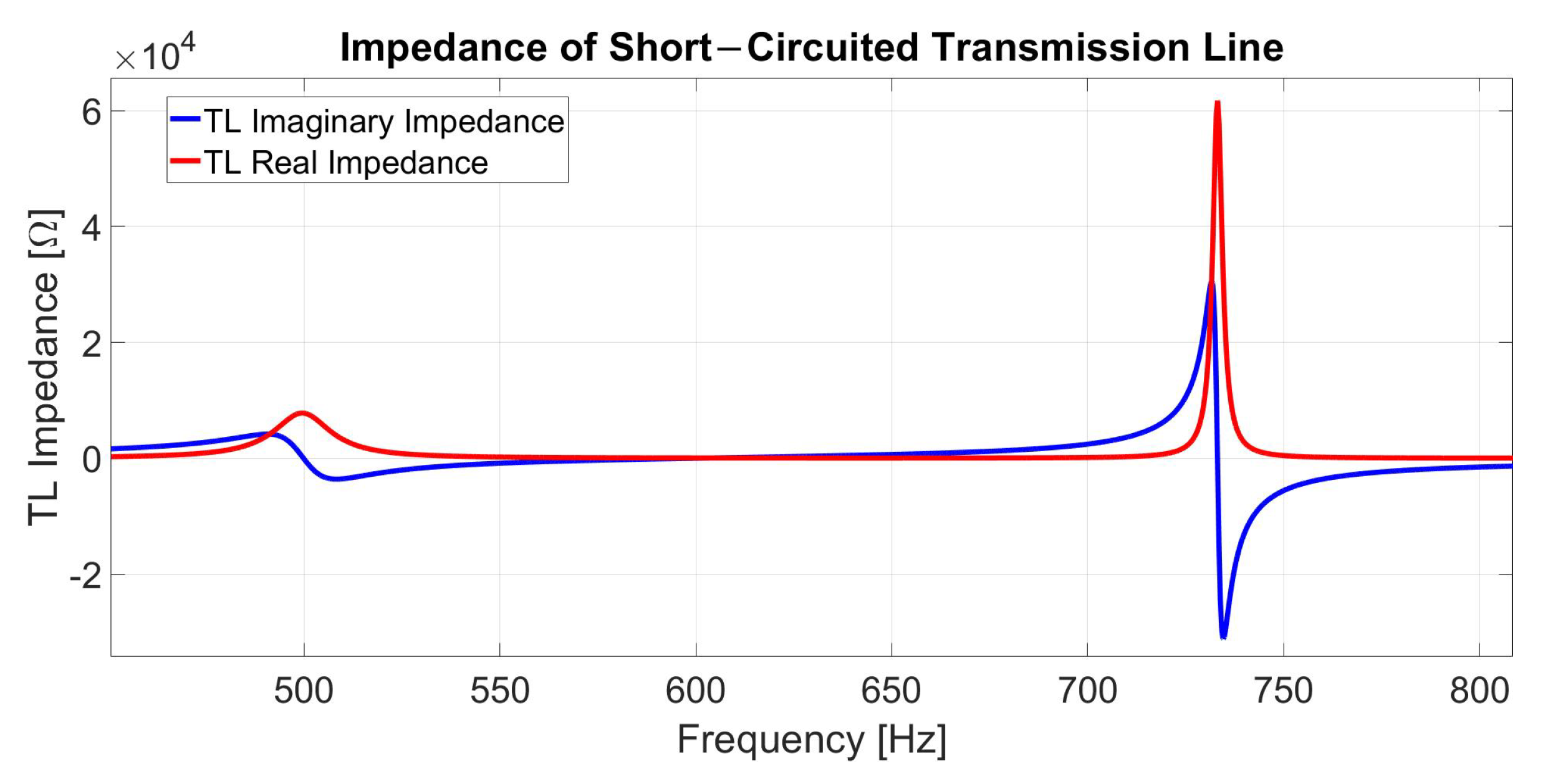
3. The Frequency Response of Transmission Lines Impedance and the Proposed Model of MTL
4. Parameters of MTLs Proposed Impedance Equation
4.1. Derivation of Resonance Equations
4.2. Model Parameters Calculation of
4.3. Model Parameters Calculation of
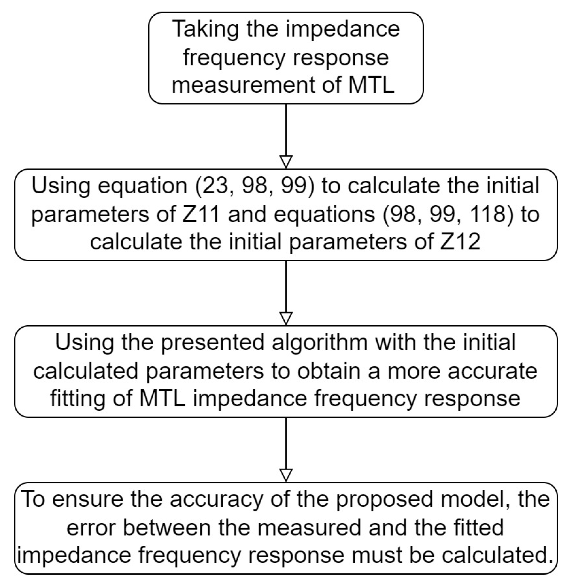
5. Developed Algorithm for an Accurate Fitting
| Algorithm 1: Developed Algorithm for an accurate model. |
|
6. Simulation Results
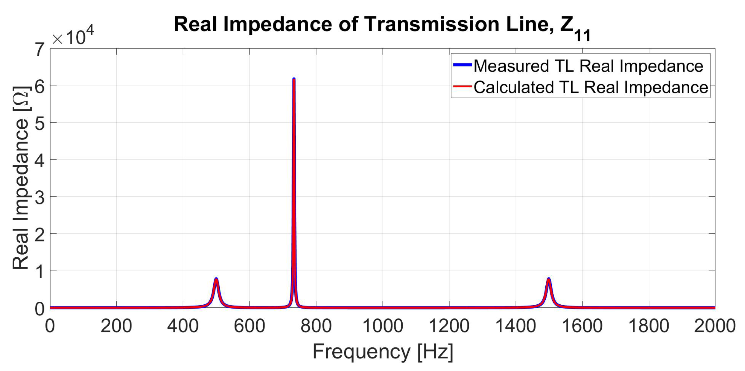
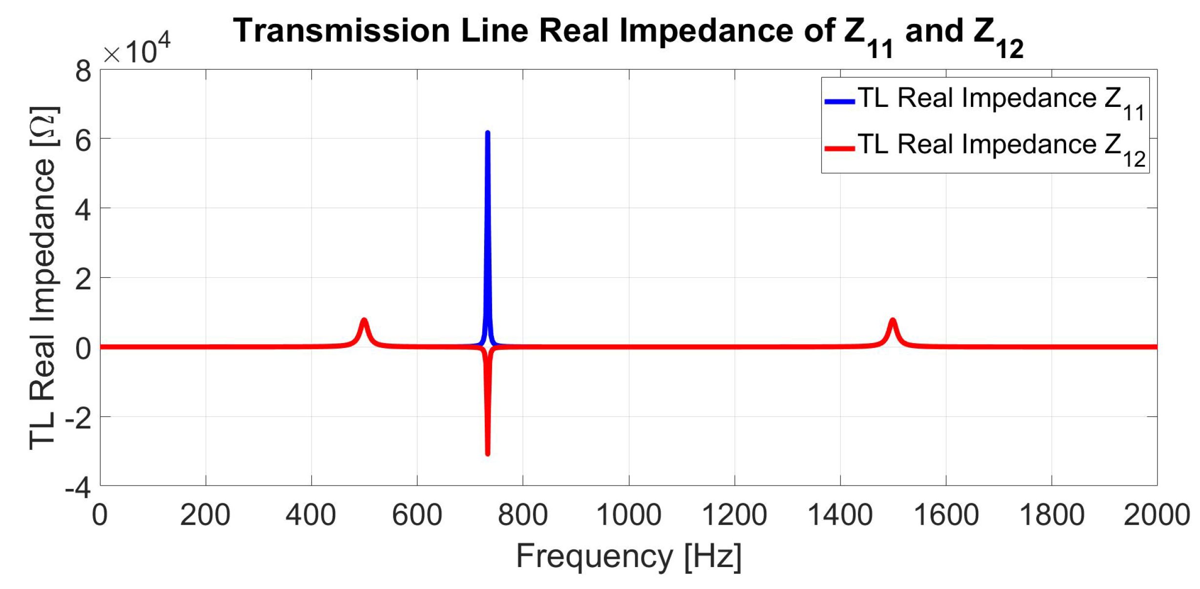
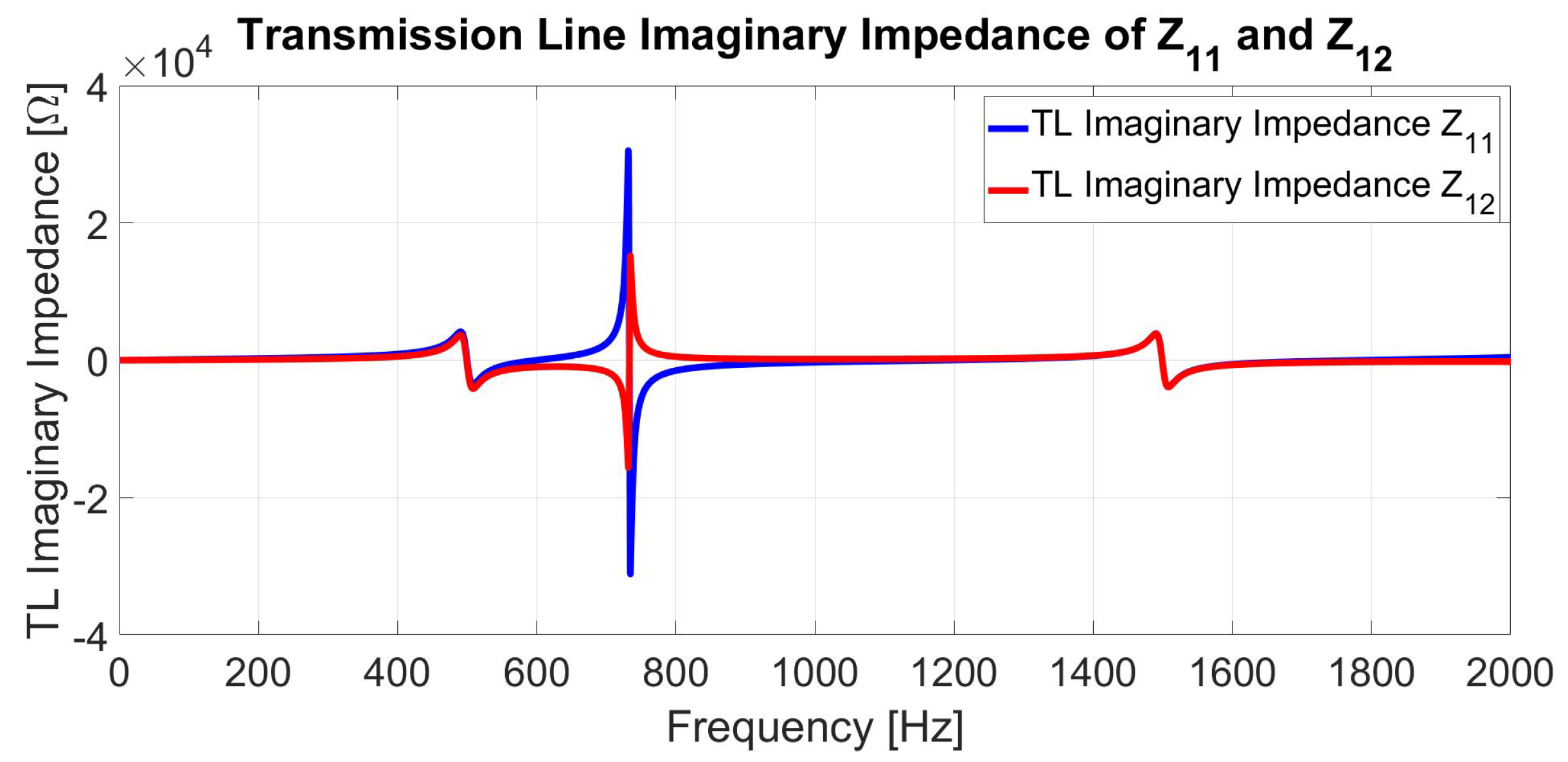
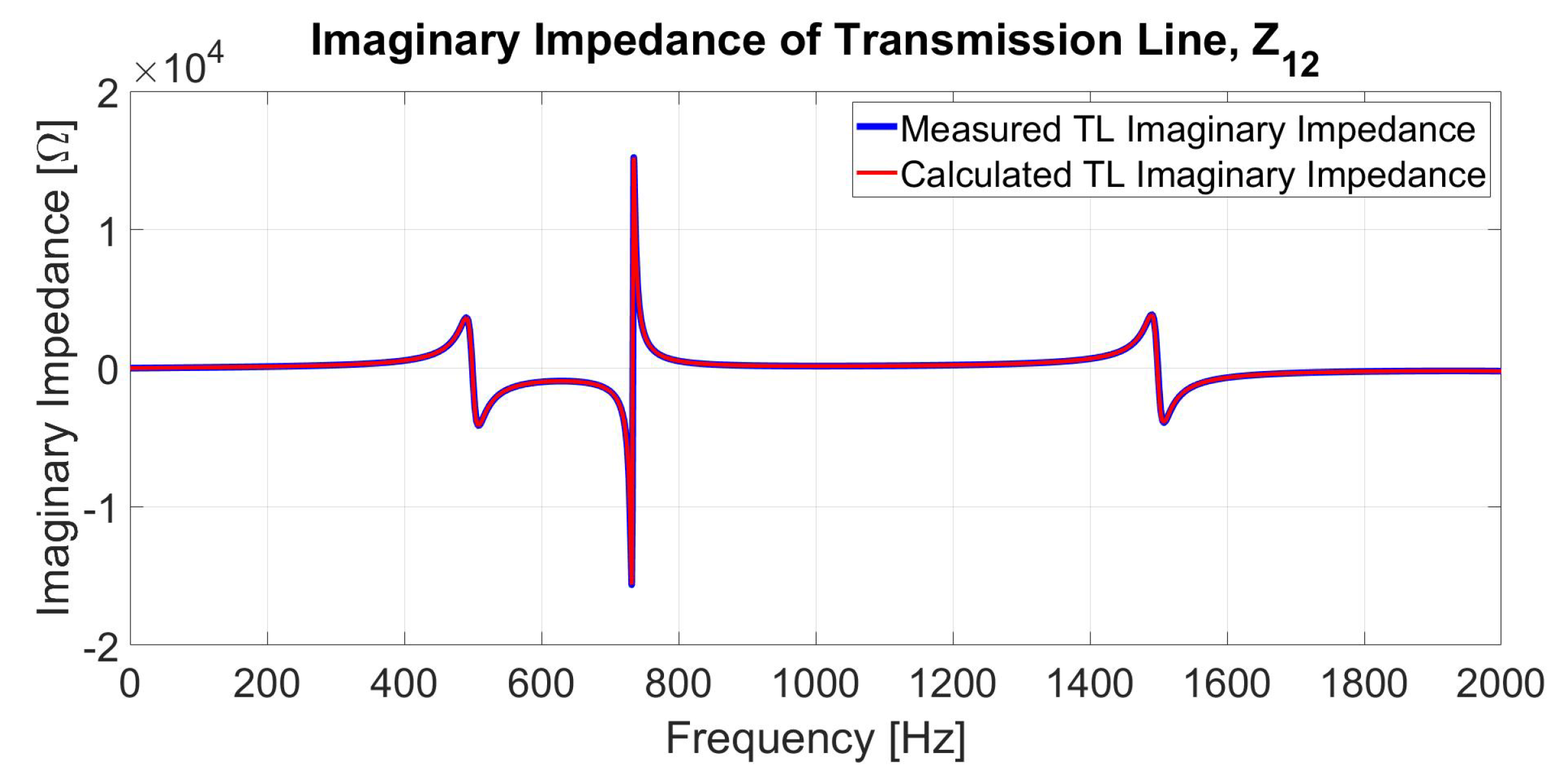
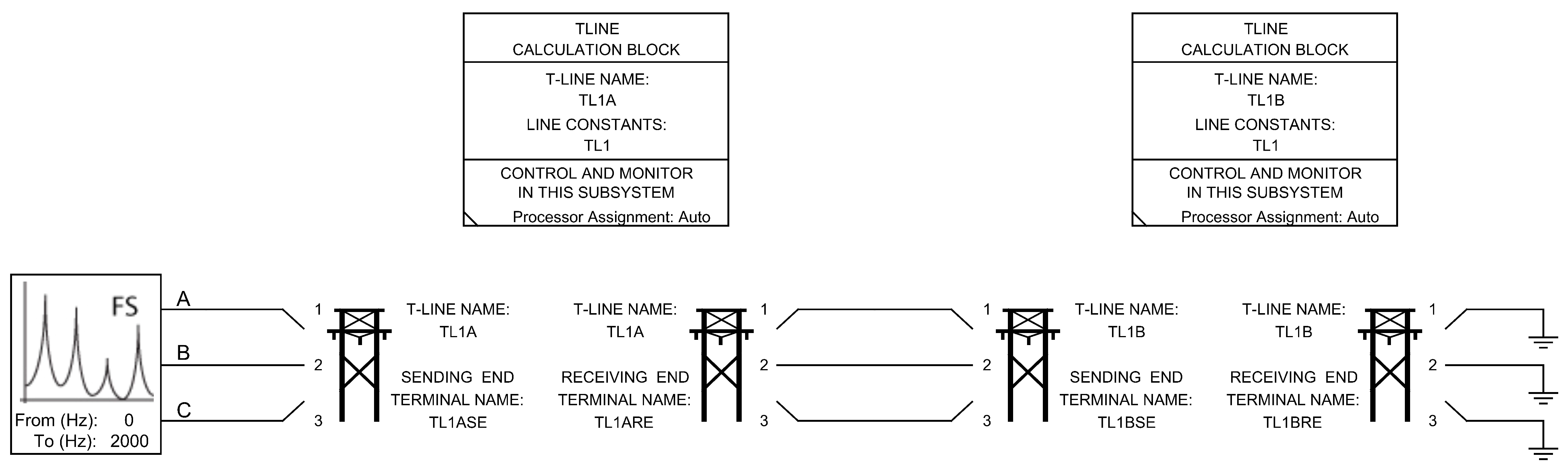
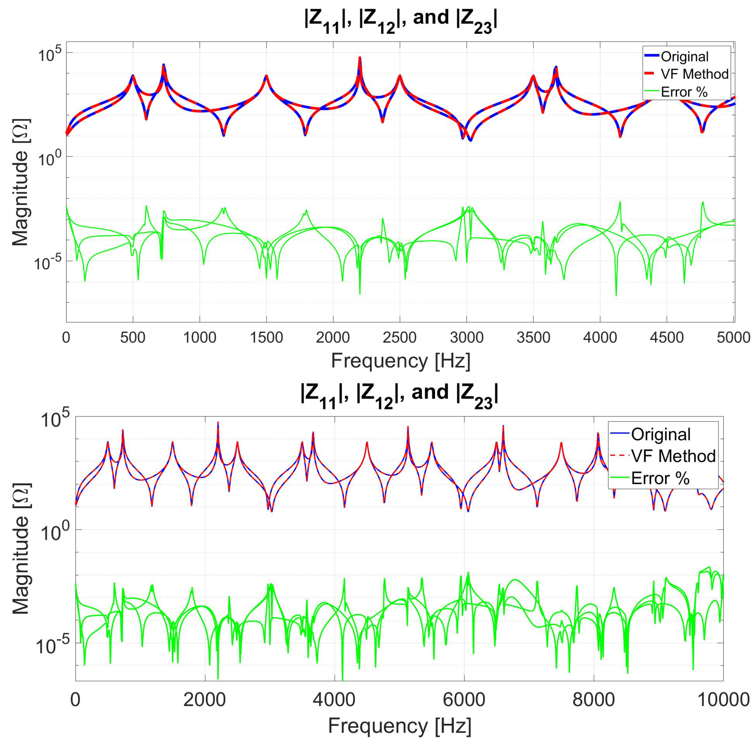
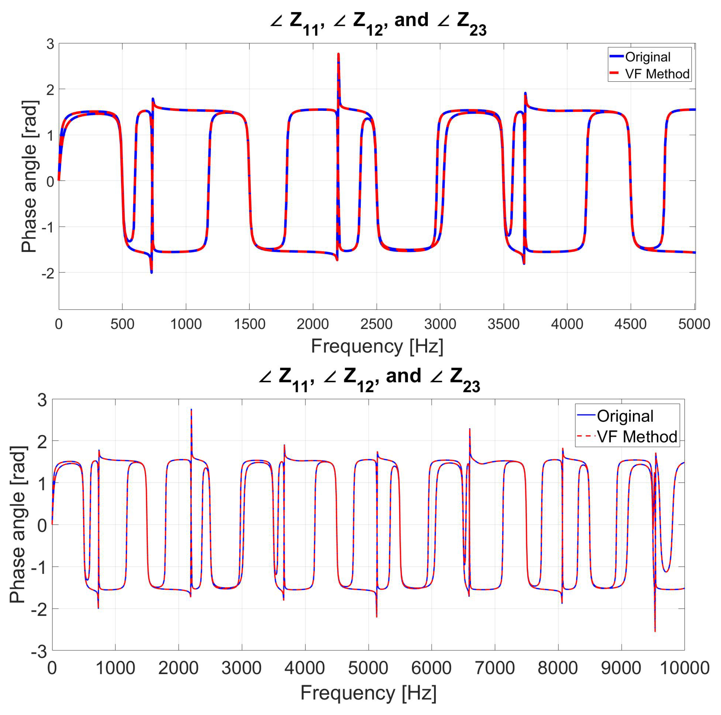
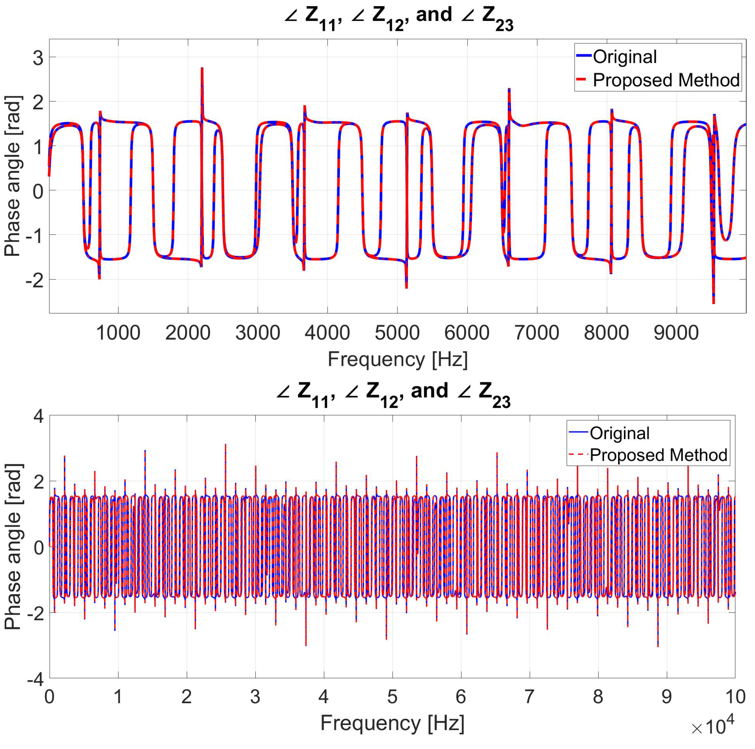
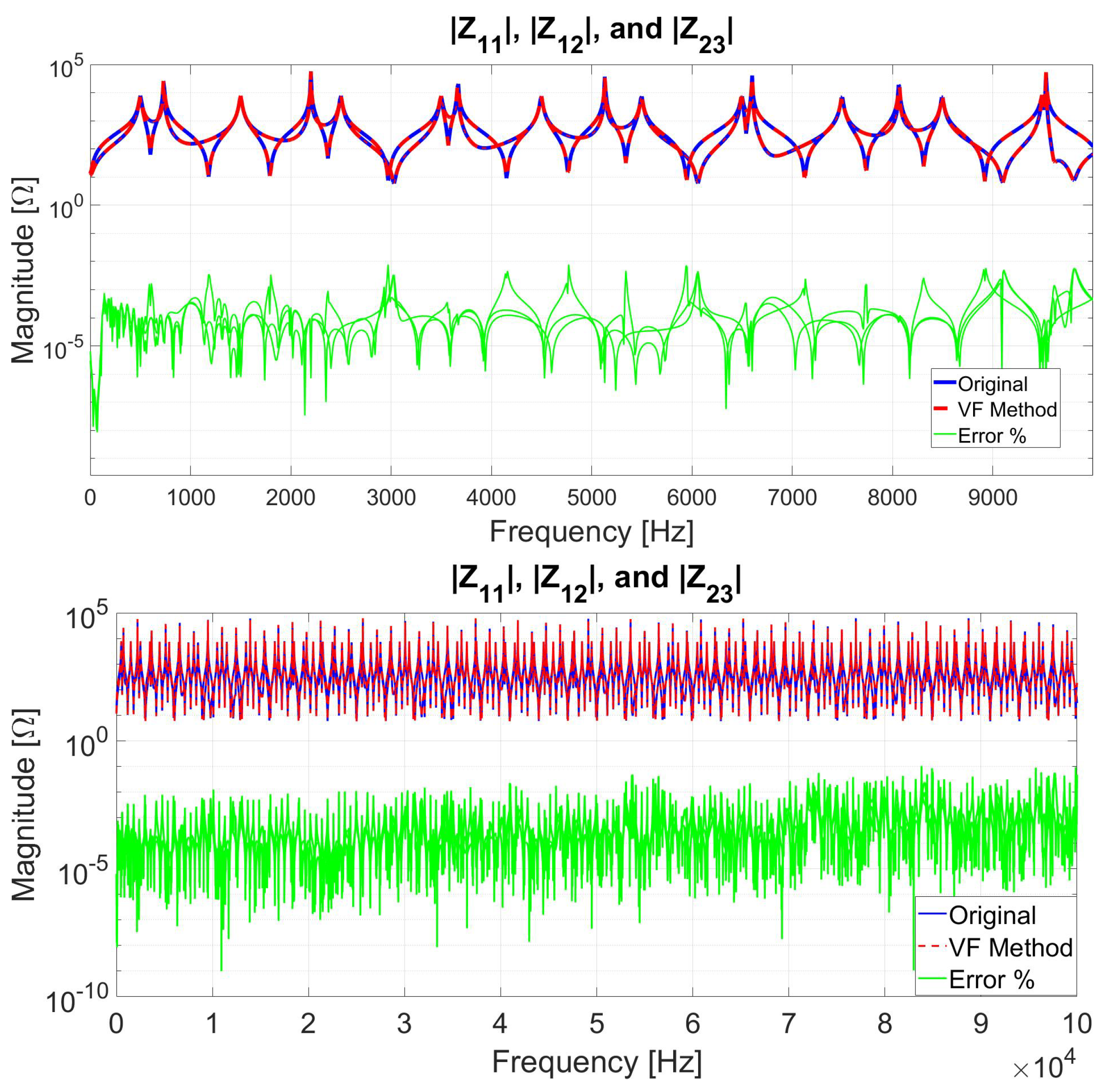
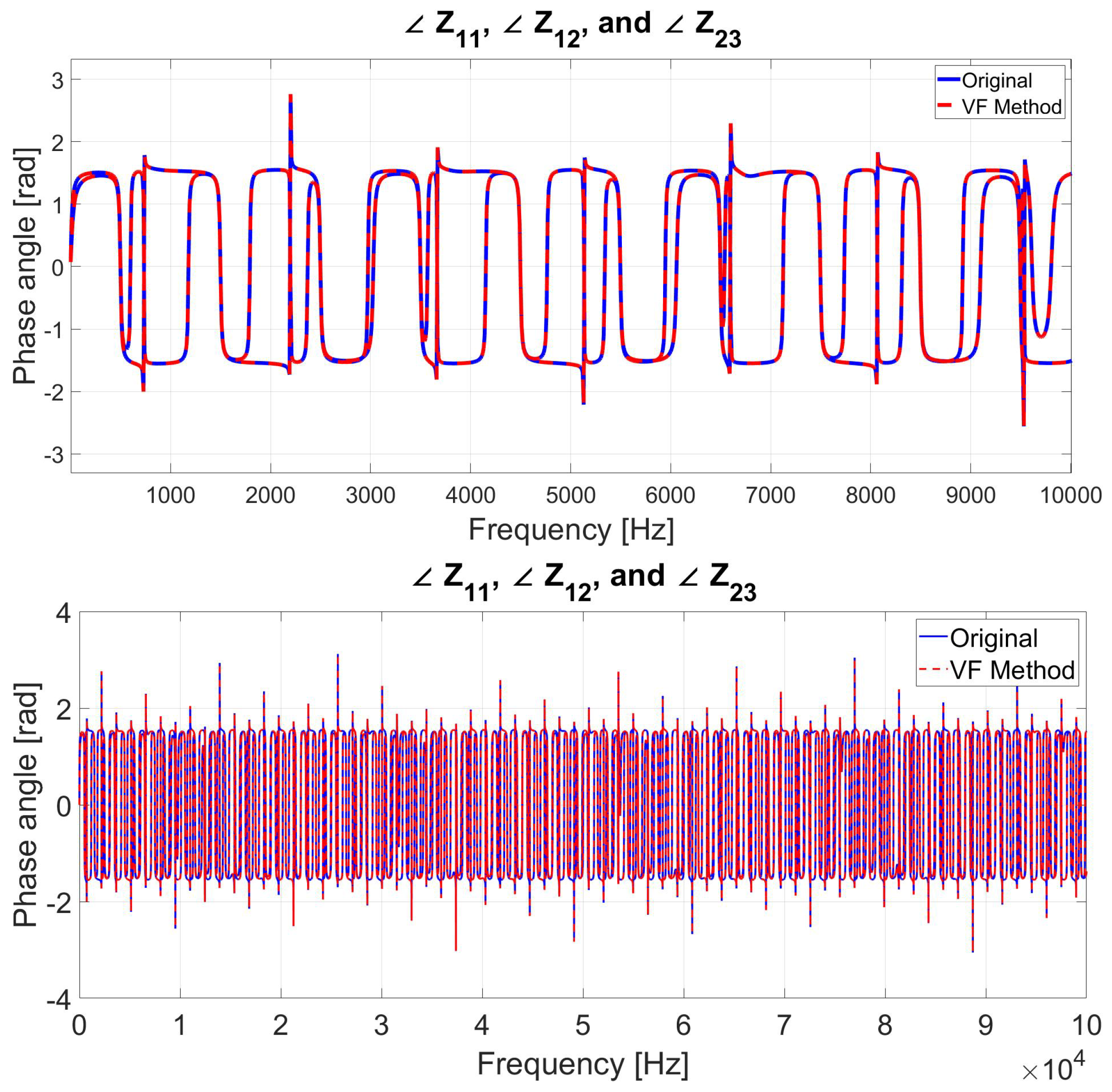
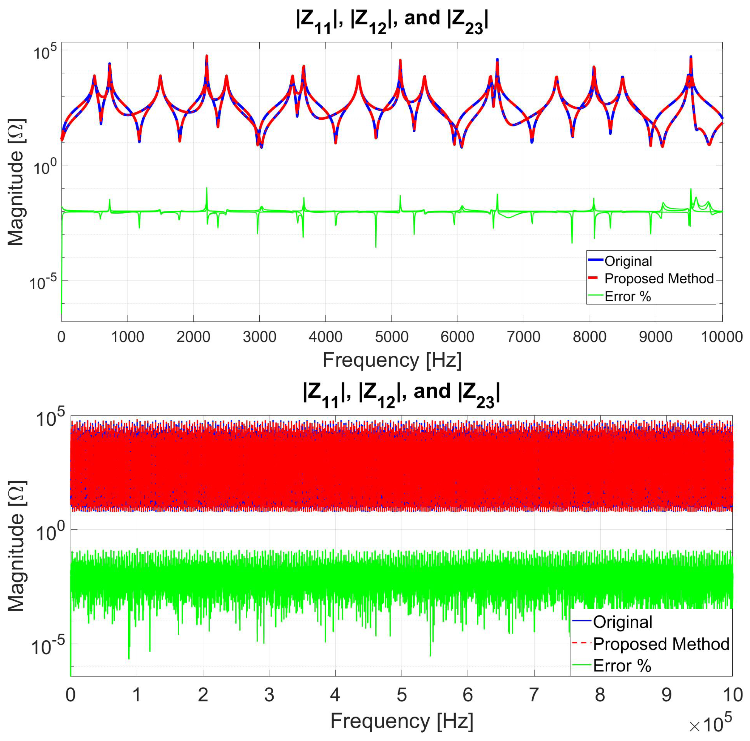
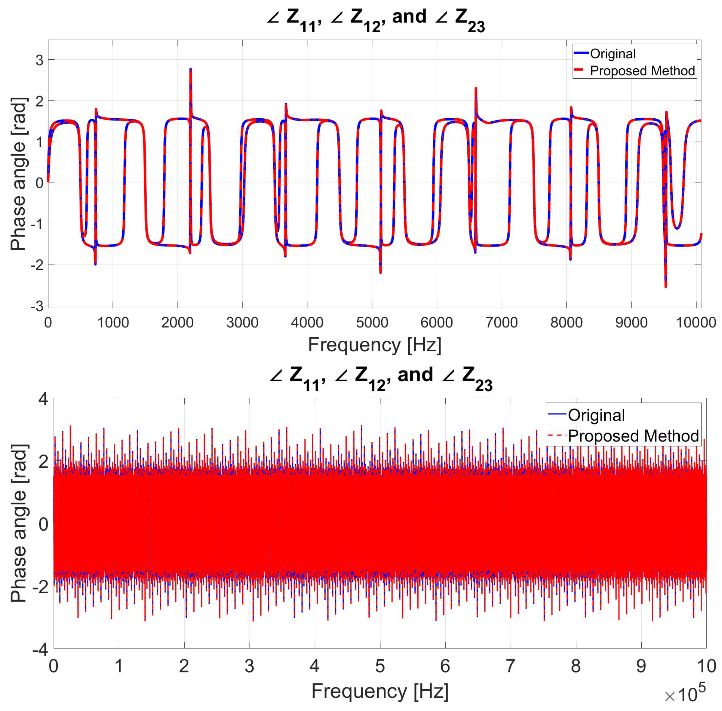
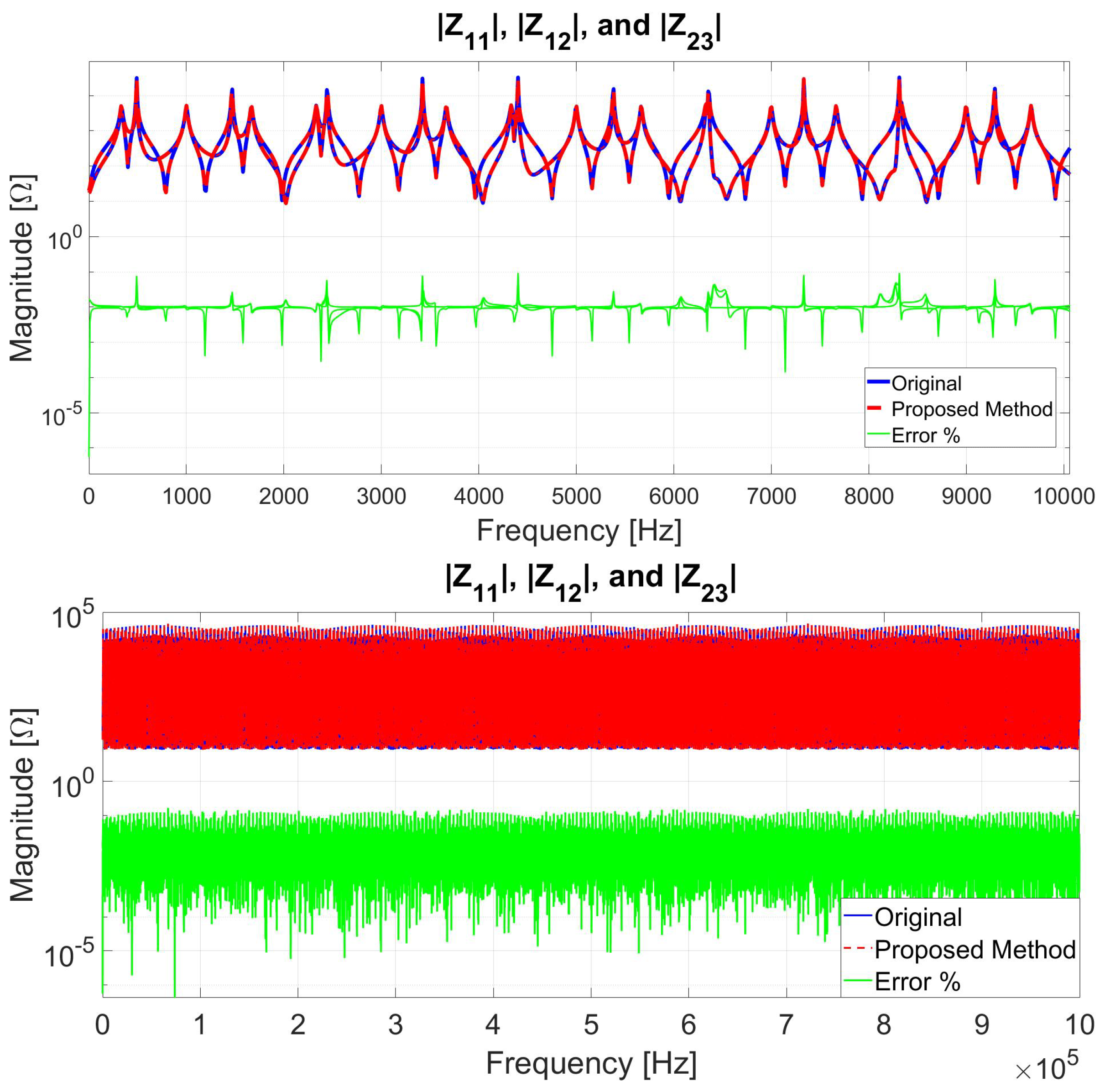
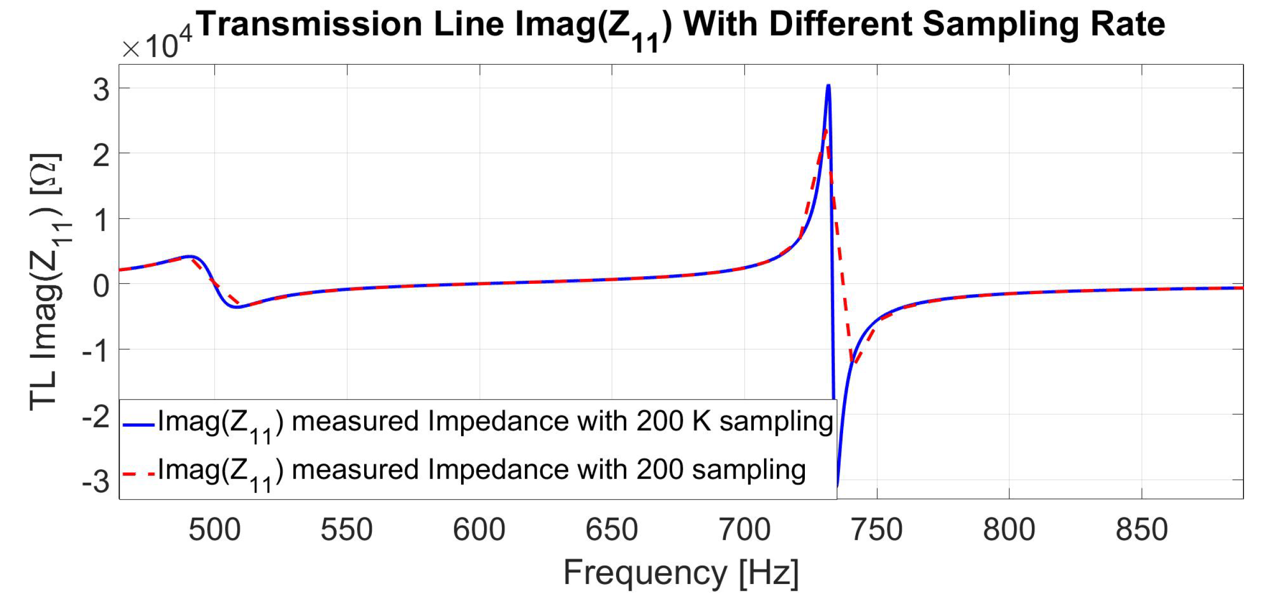
6.1. Case 1: MTL Impedance Fitting for up to 10 kHz Frequency Range
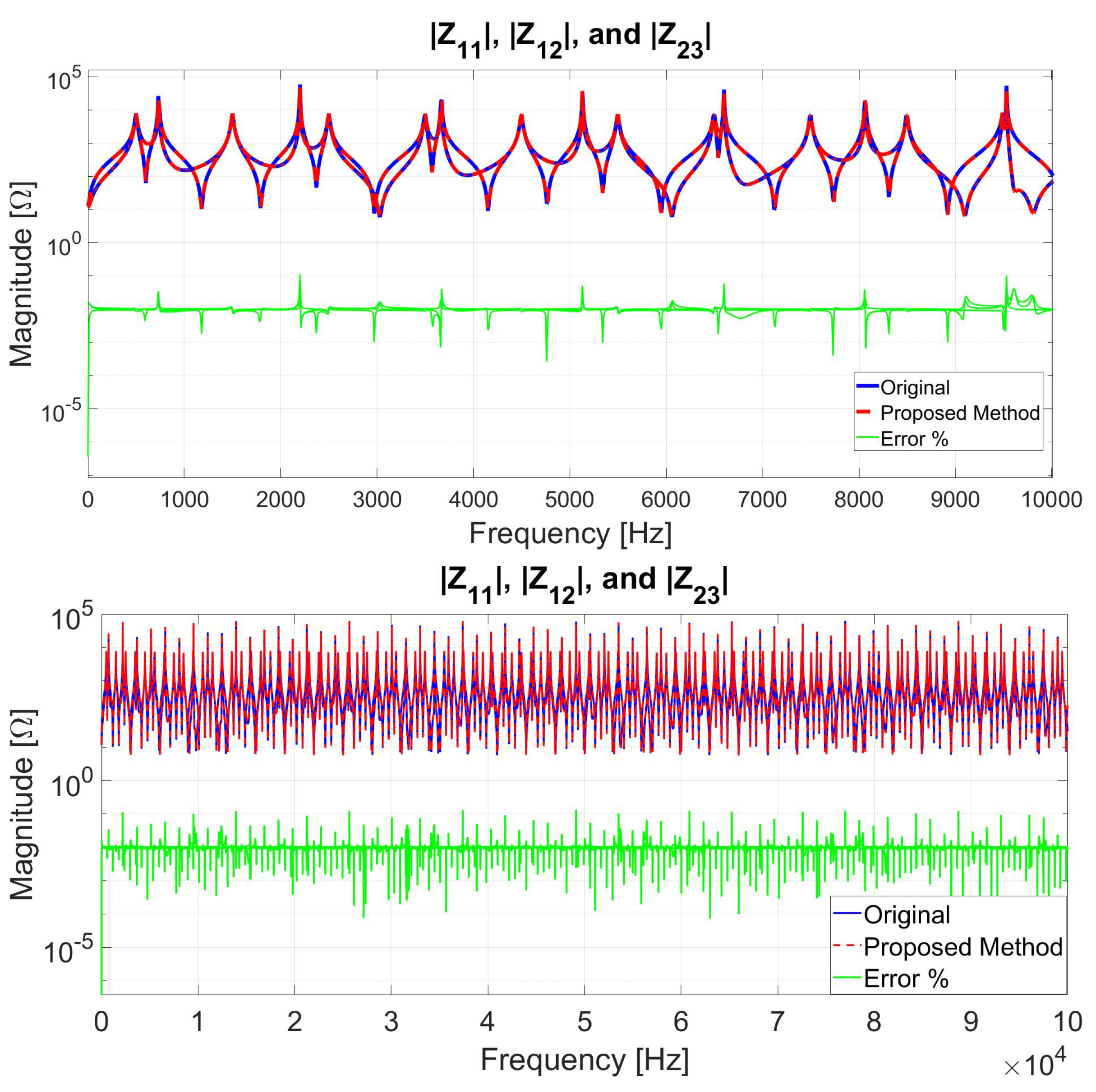
6.2. Case 2: MTL Impedance Fitting for up to 100 kHz Frequency Range
6.3. Case 3: MTL Impedance Fitting for up to 1 MHz Frequency Range
6.4. Case 4: Changing the Transmission Line Length for 1 MHz Frequency Range
6.5. Computational Time Comparison between the Proposed Method and VF
6.6. Comparison between VF and the Proposed Method
7. Features of the Proposed Method
8. Conclusions
Author Contributions
Funding
Institutional Review Board Statement
Informed Consent Statement
Data Availability Statement
Acknowledgments
Conflicts of Interest
References
- Gustavsen, B.; Semlyen, A. Rational approximation of frequency domain responses by vector fitting. IEEE Trans. Power Deliv. 1999, 14, 1052–1061. [Google Scholar] [CrossRef] [Green Version]
- Gustavsen, B.; Semlyen, A. Simulation of transmission line transients using vector fitting and modal decomposition. IEEE Trans. Power Deliv. 1998, 13, 605–614. [Google Scholar] [CrossRef]
- Gustavsen, B.; Semlyen, A. Combined phase and modal domain calculation of transmission line transients based on vector fitting. IEEE Trans. Power Deliv. 1998, 13, 596–604. [Google Scholar] [CrossRef]
- Morched, A.; Gustavsen, B.; Tartibi, M. A universal model for accurate calculation of electromagnetic transients on overhead lines and underground cables. IEEE Trans. Power Deliv. 1999, 14, 1032–1038. [Google Scholar] [CrossRef]
- Gustavsen, B. Frequency-dependent transmission line modeling utilizing transposed conditions. IEEE Trans. Power Deliv. 2002, 17, 834–839. [Google Scholar] [CrossRef]
- Ming, T.; Jianyang, S.; Jianzhao, G.; Hongjie, L.; Wei, Z.; Deliang, L. Time-Domain Modeling and Simulation of Partial Discharge on Medium-Voltage Cables by Vector Fitting Method. IEEE Trans. Magn. 2014, 50, 993–996. [Google Scholar] [CrossRef]
- Gustavsen, B.; Heitz, C. Fast Realization of the Modal Vector Fitting Method for Rational Modeling with Accurate Representation of Small Eigenvalues. IEEE Trans. Power Deliv. 2009, 24, 1396–1405. [Google Scholar] [CrossRef]
- Kocar, I.; Mahseredjian, J. Accurate Frequency Dependent Cable Model for Electromagnetic Transients. IEEE Trans. Power Deliv. 2016, 31, 1281–1288. [Google Scholar] [CrossRef]
- Ramirez, A.; Iravani, R. Enhanced Fitting to Obtain an Accurate DC Response of Transmission Lines in the Analysis of Electromagnetic Transients. IEEE Trans. Power Deliv. 2014, 29, 2614–2621. [Google Scholar] [CrossRef]
- Cervantes, M.; Kocar, I.; Mahseredjian, J.; Ramirez, A. Partitioned Fitting and DC Correction for the Simulation of Electromagnetic Transients in Transmission Lines/Cables. IEEE Trans. Power Deliv. 2018, 33, 3246–3248. [Google Scholar] [CrossRef]
- Gunawardana, M.; Kordi, B. Time-Domain Modeling of Transmission Line Crossing Using Electromagnetic Scattering Theory. IEEE Trans. Power Deliv. 2020, 35, 1020–1027. [Google Scholar] [CrossRef]
- Oh, K.S. Accurate transient simulation of transmission lines with the skin effect. IEEE Trans. Comput.-Aided Des. Integr. Circuits Syst. 2000, 19, 389–396. [Google Scholar] [CrossRef]
- Liu, X.; Cui, X.; Qi, L. Time-Domain Finite-Element Method for the Transient Response of Multiconductor Transmission Lines Excited by an Electromagnetic Field. IEEE Trans. Electromagn. Compat. 2011, 53, 462–474. [Google Scholar] [CrossRef]
- Asghari, B.; Dinavahi, V. Real-Time Nonlinear Transient Simulation Based on Optimized Transmission Line Modeling. IEEE Trans. Power Syst. 2011, 26, 699–709. [Google Scholar] [CrossRef]
- Ramirez, A.; Semlyen, A.; Iravani, R. Modeling nonuniform transmission lines for time domain simulation of electromagnetic transients. IEEE Trans. Power Deliv. 2003, 18, 968–974. [Google Scholar] [CrossRef]
- Du, Z.; Xie, Y.z.; Dong, N.; Canavero, F.G. A Spice-Compatible Macromodel for Field Coupling to Underground Transmission Lines Based on the Analog Behavioral Modeling. IEEE Trans. Electromagn. Compat. 2020, 62, 2045–2054. [Google Scholar] [CrossRef]
- Ghiasi, S.M.S.; Abedi, M.; Hosseinian, S.H. Mutually Coupled Transmission Line Parameter Estimation and Voltage Profile Calculation Using One Terminal Data Sampling and Virtual Black-Box. IEEE Access 2019, 7, 106805–106812. [Google Scholar] [CrossRef]
- Ye, H.; Strunz, K. Multi-Scale and Frequency-Dependent Modeling of Electric Power Transmission Lines. IEEE Trans. Power Deliv. 2018, 33, 32–41. [Google Scholar] [CrossRef]
- Martí, J.R.; Tavighi, A. Frequency-Dependent Multiconductor Transmission Line Model With Collocated Voltage and Current Propagation. IEEE Trans. Power Deliv. 2018, 33, 71–81. [Google Scholar] [CrossRef] [Green Version]
- Cheng, D.K. Field And Wave Electromagnetic; Addison Wesley: Boston, MA, USA, 1983. [Google Scholar]


| Advantages | Disadvantages |
|---|---|
| VF model can be used in time domain and frequency domain. | The rational function approximation is not a function in the transmission line length. |
| VF Capable of fitting the impedance to a high degree of accuracy. | The rational function approximation is a mathematical function that is not correlated to the impedance of the transmission line. Thus, it fits the data as-is. |
| VF enforces passivity to obtain a passive model. | VF required high computation power to obtain the model. |
| VF is a general mathematical model capable of fitting any physical quantity with an amplitude and angle (Vector). | The obtained model changes with the frequency range. |
| l | ||
|---|---|---|
| Inductive | ||
| Capacitive | ||
| 0 | ||
| where |
| Model | Bergeron (RLC Data Entry) |
|---|---|
| Line Length | 100 [Km] |
| Transposition | Ideally Transposed |
| Frequency | 60 [Hz] |
| Ground Resistivity | 100 [- m] |
| Number of Phases | 3 |
| Positive Sequence Series Resistance | 0.018547 [/Km] |
| Positive Sequence Series Ind. Reactance | 0.37661 [/Km] |
| Positive Sequence Shunt Cap. Reactance | 0.22789 [Meaga× Km] |
| Zero Sequence Series Resistance | 0.3618376[/Km] |
| Zero Sequence Series Ind. Reactance | 1.227747 [/Km] |
| Zero Sequence Shunt Cap. Reactance | 0.34513 [Meaga× Km] |
| Model | Bergeron (RLC Data Entry) |
|---|---|
| Line Length | 100 [Km] |
| Frequency | 60 [Hz] |
| Ground Resistivity | 100 [-m] |
| Number of Phases | 1 |
| Positive Sequence Series Resistance | 0.018547 [/Km] |
| Positive Sequence Series Ind. Reactance | 0.37661 [/Km] |
| Positive Sequence Shunt Cap. Reactance | 0.22789 [Meaga × Km] |
| Transmission Line Parameters | Calculation |
|---|---|
| 12.070792 [] | |
| 0.108695 [H] | |
| 2.304245 [F] | |
| 1.226930 [] | |
| 0.066348 [H] | |
| 1.752583 [F] |
| Transmission Line Parameters | Calculation |
|---|---|
| 12.068966 [] | |
| 0.1086480 [H] | |
| 2.3052476 [F] | |
| 0.6259449 [] | |
| 0.0335024 [H] | |
| 3.4709012 [F] |
| TL Parameters | Calculated | Fitted | Error % |
|---|---|---|---|
| 12.070792 [] | 12.06 [] | 0.0895 | |
| 0.108695 [H] | 0.108547 [H] | 0.1371 | |
| 2.304245 [F] | 2.305941 [F] | 0.0735 | |
| 1.226930 [] | 1.237722 [] | 0.8719 | |
| 0.066348 [H] | 0.066593 [H] | 0.3678 | |
| 1.752583 [F] | 1.746129 [F] | 0.3696 |
| TL Parameters | Calculated | Fitted | Error % |
|---|---|---|---|
| 12.068966 [] | 12.06 [] | 0.0743 | |
| 0.1086480 [H] | 0.108546 [H] | 0.0944 | |
| 2.3052476 [F] | 2.305959 [F] | 0.0309 | |
| 0.6259449 [] | 0.618861 [] | 1.1447 | |
| 0.0335024 [H] | 0.033297 [H] | 0.6179 | |
| 3.4709012 [F] | 3.492238 [F] | 0.6110 |
| TL Parameters | Calculated | Fitted | Error % |
|---|---|---|---|
| 12.068966 [] | 12.06 [] | 0.0743 | |
| 0.1086480 [H] | 0.108546 [H] | 0.0944 | |
| 2.3052476 [F] | 2.305959 [F] | 0.0309 | |
| 0.6259449 [] | 0.618861 [] | 1.1447 | |
| 0.0335024 [H] | 0.033296 [H] | 0.6191 | |
| 3.4709012 [F] | 3.492282 [F] | 0.6122 |
| Model | Bergeron (RLC Data Entry) |
|---|---|
| Line Length | 100 [Km] |
| Transposition | Ideally Transposed |
| Frequency | 60 [Hz] |
| Ground Resistivity | 100 [-m] |
| Number of Phases | 3 |
| Positive Sequence Series Resistance | 0.018547 [/Km] |
| Positive Sequence Series Ind. Reactance | 0.37661 [/Km] |
| Positive Sequence Shunt Cap. Reactance | 0.22789 [Meaga × Km] |
| Zero Sequence Series Resistance | 0.3618376[/Km] |
| Zero Sequence Series Ind. Reactance | 1.227747 [/Km] |
| Zero Sequence Shunt Cap. Reactance | 0.34513 [Meaga × Km] |
| Computer | Specs |
|---|---|
| RAM | 32 GB, 3200 MHz |
| CPU | i7-11700F |
| Operating system | Windows 11 |
| Method | Computational Time [S] |
|---|---|
| VF | 24,663.37 |
| Proposed Model | 516.75 |
| Frequency [kHz] | Number of Parameters | Computational Power | ||
|---|---|---|---|---|
| Vector Fitting | Proposed Model | Vector Fitting | Proposed Model | |
| 10 | 50 | 24 | Low | Low |
| 100 | 750 | 24 | Medium | Low |
| 1000 | NA | 24 | High | Low |
Publisher’s Note: MDPI stays neutral with regard to jurisdictional claims in published maps and institutional affiliations. |
© 2022 by the authors. Licensee MDPI, Basel, Switzerland. This article is an open access article distributed under the terms and conditions of the Creative Commons Attribution (CC BY) license (https://creativecommons.org/licenses/by/4.0/).
Share and Cite
Alharbi, H.; Khalid, M.; Abido, M. Transmission Lines Impedance Fitting Using Analytical Impedance Equation and Frequency Response Analysis. Mathematics 2022, 10, 2677. https://doi.org/10.3390/math10152677
Alharbi H, Khalid M, Abido M. Transmission Lines Impedance Fitting Using Analytical Impedance Equation and Frequency Response Analysis. Mathematics. 2022; 10(15):2677. https://doi.org/10.3390/math10152677
Chicago/Turabian StyleAlharbi, Hosam, Muhammad Khalid, and Mohammad Abido. 2022. "Transmission Lines Impedance Fitting Using Analytical Impedance Equation and Frequency Response Analysis" Mathematics 10, no. 15: 2677. https://doi.org/10.3390/math10152677
APA StyleAlharbi, H., Khalid, M., & Abido, M. (2022). Transmission Lines Impedance Fitting Using Analytical Impedance Equation and Frequency Response Analysis. Mathematics, 10(15), 2677. https://doi.org/10.3390/math10152677