Article

Visualizing a Cubic Linkage through the Use of CAS and DGS

1
Departamento de Ingeniería Industrial, Escuela Politécnica Superior, Universidad Antonio de Nebrija, 28015 Madrid, Spain
2
Sociedad Asturiana de Educación Matemática “Agustín de Pedrayes”, Federación Española de Sociedades de Profesores de Matemáticas, 33213 Gijón, Spain
3
Departamento de Matemáticas, Estadística y Computación, Universidad de Cantabria, 39008 Santander, Spain
4
CEAD Profesor Félix Pérez Parrilla, 35005 Las Palmas de Gran Canaria, Spain
*
Author to whom correspondence should be addressed.
These authors contributed equally to this work.
Mathematics 2022, 10(15), 2550; https://doi.org/10.3390/math10152550
Submission received: 22 June 2022 / Revised: 18 July 2022 / Accepted: 20 July 2022 / Published: 22 July 2022
(This article belongs to the Special Issue Symbolic Computation for Mathematical Visualization)

Abstract

:
Our goal is to discuss the different issues that arise when attempting to visualize a joints-and-bars cube through GeoGebra, a widespread program that combines dynamic geometry (DGS) and computer algebra systems (CAS). As is standard in the DGS framework, the performance of the graphic model (i.e., the positions of the other vertices when dragging a given one) must correspond to a mathematically rigorous, symbolic computation-driven output. This requirement poses both computational algebraic geometry and dynamic geometry programming challenges that will be described, together with the corresponding proposed solutions. Among these, we include a complete determination of the dimension of the cubic linkage from an algebraic perspective, and introduce advanced 3D visualizations of this structure by using the GeoGebra software.
MSC:
51-08; 51M15; 14P05; 14Q30; 70-10

1. Introduction

Dynamic geometry software (DGS) programs, such as Cabri, The Geometer’s Sketchpad, Cinderella or GeoGebra, were initially conceived as a tool for teaching geometry in schools, as a digital assistant for the constructions traditionally made by ruler and compass on a notebook or the blackboard.
As is well known, geometric reasoning on ruler and compass constructions requires developing logical arguments beyond their mere visual appearance: it is not admissible to conclude, for example, that some lines on a figure are parallel just because of their appearance. A geometric construction is not just a drawing, but a set of instructions whose output delivers a geometric figure with a definite list of geometric properties. This fact is emphasized when using DGS programs, as dragging figures—one of the five essential features in the DGS paradigm, together with dynamic transformation, measurement, animation and locus computation capabilities (see, for instance, [1,2] or [3])—helps to identify those properties of the constructions that are mathematically intrinsic, and to discard those that are just visually accidental.
In recent times, the development of DG software has incorporated powerful new features, such as embedded computer algebra systems (CAS) that help perform symbolic computations, providing a sound algebraic foundation on which these geometric constructions are built. This represents, at least from a formal point of view, an improvement over previous DGS that only used numerical methods to produce their outputs. As an example, the DGS GeoGebra incorporates in its latest versions a CAS based on the Giac platform [4,5], which can be accessed from the CAS view of the program. Since symbolic computations can be complex and lengthy in certain situations, GeoGebra uses a mixed approach when confronting geometric constructions, taking advantage of both the faster numerical algorithms on the one hand, and the precision offered by a symbolic approach on the other hand (often when requested from the user through the use of specific commands).
The set of tools provided by DGS, always increasing in ease of use, variety and powerfulness, allows us to also successfully confront the task of creating models representing complex geometric objects. The importance of making physical models of geometric objects has been widely emphasized [6], and the current digital revolution is providing new ways of virtualizing these physical models in order to facilitate their study and accessibility (with an extra advantage of reducing costs). As an excellent showcase of virtual geometric models, the reader is referred to Imaginary [7], an open-source project that defines itself as a non-profit organisation for the communication of modern mathematics. Returning to DGS and GeoGebra, with a quick search in its repository of resources, one can find a great variety of geometric models related to diverse fields, such as architecture, biology, physics, engineering, etc. The inclusion of a 3D engine to create spatial models after the release of GeoGebra 5.0 bolstered their production, mostly (but not only) designed with educational purposes in mind.
In this article, we concern ourselves with the modeling of linkages (as defined, for example, in [8] or [9]) through the use of DGS, as well as the study of their geometric and algebraic properties with the assistance of a CAS. Linkages constitute a family of geometric objects of current interest in diverse fields of research, often connected with the design of a variety of structures such as robotic mechanisms, manufacturing processes, architectural frames, molecular arrangements, etc. Here, we will focus our attention on a specific structure: the cubic linkage. By the cubic linkage, we understand a spatial linkage formed by the vertices and rigid edges that constitute the frame of the regular cube (see Figure 5 in Section 2.2.4). To economize the language used throughout the text, we will often refer to any 3-dimensional realization of this linkage simply as a cube. In order to settle some conventions, we will always assume that the cube has edges of 1 unit length. Even though this cubic linkage is quite a natural structure to take into consideration, it is surprising to observe the scarce information that can be found about it. We will see in the sequel the difficulties that arise when trying to fully understand its geometry, even with powerful mathematical software such as Maple. Indeed, two of the authors already approached the study of this elusive structure in a previous work [10], stating some open questions which we partially solve here.
In Section 2, we settle the mathematical model for our treatment of linkages immersed in a Euclidean space, which will have a strong algebraic flavour since we will associate with a linkage an algebraic (non-necessarily irreducible) variety. We establish basic definitions, introduce initial examples, and comment on certain advantages and limitations of our approach. In Section 3, we carefully study the geometric and algebraic properties of the cubic linkage, determining the dimension of its associated variety. Then, in Section 4, after discussing some issues concerning the visualization of linkages in DGS, we proceed to describe some of the visual, dynamic models we have developed in GeoGebra to simulate the cube in a 3D environment. Finally, we conclude by presenting how our approach contributes to answering a number of questions posed in [10]. These questions spurred our interest to delve deeper into this structure, which to us represents a real challenge both to completely understand its underlying algebraic structure as well as to visually modelize it through the use of DGS.

2. A Mathematical Model for Linkages

2.1. Selection of the Model

Traditionally, whenever finding an object with mathematical properties in a given field of knowledge, the need quickly arises to build an appropriate model that grasps its essential mathematical features and allows a deeper understanding of the laws governing its behavior. However, this task of modelizing a given piece of reality is rather a subtle question that can be addressed from many different points of view and with diverse mathematical tools. On the other hand, during the development of new mathematical ideas, scientists also attempt to model these new abstract entities to give them a physical presence and make them more comprehensible. As an example of the latter approach, we can mention [6], where the discovery of new surfaces and curves during the 19th century led to a widespread interest in constructing physical models to visualize and understand their properties.
With the advent of the digital era, the new trends in modeling often moved from the physical world to the virtual space, and computers became a new sandbox to recreate either physical or mathematical objects. We can see this transition from physical models to digital ones across all technical and scientific disciplines, as well as in the educational context (see [11] for an account of the transition from analogue to digital devices in the classroom).
In this paper, our object of interest comes originally from a family of mechanisms which are usually referred to as linkages. A linkage is a mechanical device consisting a a finite set of rigid bars, some of which are connected at their extremes in a free-to-move joint (see Figure 1).
Usually, linkages are considered on the plane or in 3-dimensional space. For the mathematically oriented person, the need quickly arises to give a mathematical definition for this family of devices, so that its properties can be better understood. That is, we are in need of a mathematical model to pursue our investigation.
Before providing a definition, we start by setting up some notation and basic concepts. Given two points, v 1 and v 2 , in Euclidean space, we denote by v 1 v 2 their Euclidean distance—that is, the length of the segment joining them. By a graph we understand a pair G = ( V , E ) consisting of a finite set of elements V = { v 1 , , v r } called vertices and a subset E of the set of 2 combinations of V. Each element of E is called an edge of the graph G, and the 2-combination { v i , v j } is denoted by e i j (through this work, not more than 8 vertices will be considered altogether, so that the corresponding sub-indices will always be one-digit numbers and no confusion will arise with this notation). The following is a common definition for linkages (see for example [9]), although some variations on terminology can be found in the literature.
Definition 1.
Let G = ( V , E ) denote a graph with r vertices. An abstract linkage L for the graph G is a pair ( G , l ) , where l : E R + is a map assigning to each edge e i j E a positive real number l ( e i j ) l i j , which we call its length. A realization in R n of an abstract linkage L = ( G , l ) is a pair ( L , ψ ) , where ψ : V R n satisfies ψ ( v i ) ψ ( v j ) = l i j for each edge e i j E (in this notation we will always assume i < j ).
Some of the fundamental problems that arise when dealing with these mathematical objects concern diverse topological and geometrical questions:
1.
(Existence) For which abstract linkages does there exist a realization in R n ?
2.
(Rigidity) Which abstract linkages admit just one realization in R n up to congruence?
3.
(Configuration space) How is the space of all possible realizations of an abstract linkage? What is its dimension, topology…?
There are diverse mathematical tools to approach these problems that come from diverse fields such as mechanics, differential geometry, combinatorics, topology or algebraic geometry. In particular, the algebraic geometry approach comes from the fact that the conditions ψ ( v i ) ψ ( v j ) = l i j can be expressed by means of quadratic polynomials, so that we can express a realization of an abstract linkage by means of a set of polynomials in the coordinates of ψ ( v i ) , i = 1 , , n . In this work, we will adopt this perspective for dealing with linkages, an approach that involves—because of the great level of development and higher simplicity of algebraic geometry over algebraically closed fields, as mentioned in the quotation below—the parallel consideration, in many instances, of linkage realizations in C n in order to derive properties for the R n context. For the cube linkage we initially have 8 vertices connected by 12 unit-length rods, and so the algebraic model consists of 8 · 3 = 24 variables and 12 quadratic equations defining the distances among them. To see the kind of difficulties that can (and will) arise when dealing with this model for the cube, it is worthwhile to quote here [12]:
Since (squared) distance constraints satisfied by the joint coordinates are given by quadratic polynomials, it is possible to try to analyze the set of all realizations of a given pair ( G , l ) symbolically using computational algebra. However, a Gröbner basis for an ideal generated by quadratic polynomials in k variables can require generators of degree O ( 2 2 k ) so computations with the squared distance constraints may quickly become intractable. Moreover, care must be taken in applying results from algebraic geometry in this setting as we are interested in realizations over the real numbers, and many results in algebraic geometry require an algebraically closed ground field.
To each abstract linkage L we can associate the variety of its realizations in R n . If L has r vertices v 1 , … , v r and, having in mind that each vertex v i has n coordinates ( x i 1 , , x i n ) , this variety lives in ( R n ) r R n r and is determined by a set of s polynomial equations p i ( x 11 , , x r n ) = 0 , p i R [ x 11 , , x r n ] , given by the conditions on the lengths of its edges. With the language of algebraic geometry, if I ( L ) = p 1 , , p s R [ x 11 , , x r n ] denotes the ideal generated by the polynomials p i , then the variety of realizations is V ( I ( L ) ) . As mentioned above, since working with an algebraically closed field facilitates certain computations and simplifies some arguments that will arise in the sequel, we establish the following definitions to define the mathematical model for linkages that we will be using throughout the present work.
Definition 2.
Let L be an abstract linkage with r vertices V = { v 1 , , v r } and s edges E = { e i j } of lengths l i j . Let us associate with each v i the n-tuple of variables ( x i 1 , , x i n ) , and with each edge e i j in E the polynomial
p i j ( x i 1 , , x i n , x j 1 , , x j n ) = k = 1 n ( x j k x i k ) 2 l i j 2 .
The free n-linkage V n ( L ) is the variety in ( C n ) r determined by the ideal in C [ x 11 , , x r n ]
I n ( L ) = p i j R [ x 11 , , x r n ] : e i j E
Now, given a finite collection of polynomials Q = { q 1 , , q s } R [ x 11 , , x r n ] , the semi-free n-linkage V n ( L , Q ) is the variety determined by the ideal I n ( L , Q ) generated by the polynomials p i j , the same ones that generate the free n-linkage, plus the polynomials in Q. These extra polynomials are called the restrictions of the semi-free linkage. Whenever the dimension n of the ambient space R n is clear from the context we will use simply the word linkage to refer to a semi-free n-linkage. A C -realization of an either free or semi-free linkage is a point of the corresponding (complex) variety. A R -realization (or simply realization) of a linkage is a C -realization with real coordinates.
From these definitions, it readily follows that in fact, a semi-free n-linkage for the abstract linkage L is nothing else than a subvariety of the free n-linkage V n ( L ) .
Remark 1.
In order to clarify the relationship between one vertex and the variables representing its coordinates, when working with 2-linkages (3-linkages), we will often name a vertex with a capital letter such as A and its corresponding coordinates by A x , A y ( A z ).
Definition 3.
Two realizations R L = ( t 11 , , t r n ) and R L = ( t 11 , , t r n ) of an n-linkage L with r vertices are congruent if and only if there is an isometry ϕ : R n R n such that ϕ ( t k 1 , , t k n ) = ( t k 1 , , t k n ) for k = 1 , , r . If ϕ is a direct (inverse) isometry, we say that R L and R L are directly (inversely) congruent.
In other words, two realizations of a linkage are congruent if there is an isometry taking one bijectively onto the other, preserving the labeling of the vertices. Therefore, even though two realizations can be isometric under relabelling of their vertices, they will not be considered congruent here (see Figure 2).
Example 1.
Let us consider the abstract linkage L 1 corresponding to a graph with three vertices { A , B , C } and the three edges joining them, see Figure 3. Assume each edge is given length 1. Let us describe the free 2-linkage for this abstract linkage. If we set A = ( A x , A y ) , B = ( B x , B y ) , C = ( C x , C y ) , then
V 2 ( L 1 ) = { ( A x , A y , B x , B y , C x , C y ) C 6 : ( B x A x ) 2 + ( B y A y ) 2 1 = 0 , ( C x B x ) 2 + ( C y B y ) 2 1 = 0 , ( A x C x ) 2 + ( A y C y ) 2 1 = 0 }
The variety V 2 ( L 1 ) is contained in C 6 and is determined by the ideal
I 2 ( L 1 ) = ( B x A x ) 2 + ( B y A y ) 2 1 , ( C x B x ) 2 + ( C y B y ) 2 1 , ( A x C x ) 2 + ( A y C y ) 2 1 ,
which corresponds to the 3 conditions determined by the lengths of its edges. The expected dimension of this variety should be 6 3 = 3 . We proceed to check this with Maple:
>
with(PolynomialIdeals):
>
IL1:=<(Bx − Ax)^2 + (By − Ay)^2 − 1, (Cx − Bx)^2 + (Cy − By)^2 − 1,
(Ax − Cx)^2 + (Ay − Cy)^2 − 1>
>
HilbertDimension(IL1)
3
This result is valid at least over C 6 , since over the complexes there is a correspondence between the dimension of an ideal and the geometric dimension of its zero-set. Yet, it is easy to check that I ( L 1 ) is a real ideal by considering the Jacobian and checking that it has rank 6 3 = 3 . On the other hand, we will later see how this naïve approach to guess dimensions will often lead to unexpected results.
Since the group of Euclidean isometries Iso ( R 2 ) of the plane is also a 3-dimensional variety (see Theorem 1 in [13], where the variety of isometries is studied over the reals, concluding that the standard definition of isometry provides a real ideal, with properties similar to the well-known ones in the complex setting), in order to reduce the number of variables that come into play and focus our attention just on internal changes of configuration of our linkage, we can proceed now to fix two of the vertices of the triangle (let us say A = ( A x , A y ) ( 0 , 0 ) and B = ( B x , B y ) ( 1 , 0 ) ) and study all possible configurations for the semi-free linkage V 2 ( L 1 , Q 1 ) , where Q 1 = { A x , A y , B x 1 , B y } . The corresponding ideal is I 2 ( L 1 , Q 1 ) = I 2 ( L 1 ) + A x , A y , B x 1 , B y and has four restrictions, leaving us in fact with only two variables C x , C y and two equations ( C x 1 ) 2 + ( C y 0 ) 2 1 = 0 , ( 0 C x ) 2 + ( 0 C y ) 2 1 = 0 , so that now the expected dimension should be 0:
>
with(PolynomialIdeals):
>
ILQ1:=<(Bx − Ax)^2 + (By − Ay)^2 − 1, (Cx − Bx)^2 + (Cy − By)^2 − 1,
(Ax − Cx)^2 + (Ay − Cy)^2 − 1, Ax, A_y, B_x − 1, B_y>
>
HilbertDimension(ILQ1)
0
the fact that a variety has dimension zero translates into the fact that there is only a finite number of possible realizations (or none at all). To answer which are these possible realizations, we can ask Maple to find all possible solutions for the corresponding system of equations:
>
solve(Generators(ILQ1), {Cx, Cy})
Cx = 1 2 , Cy = RootOf Z 2 3 2
this output corresponds to the two possible equilateral triangles with vertices ( 0 , 0 ) , ( 1 , 0 ) and 1 2 , ± 3 2 . Notice that these two solutions are congruent; we will later see that this situation corresponds to a globally rigid linkage in R 2 (see Section 2.2.1 below).

2.2. Some Issues concerning the Model

Before providing more examples of linkages and proceeding to a careful study of the cube, it is interesting to make some observations with respect to our chosen mathematical model, including how to deal in this framework with key concepts such as that of rigidity and with some shortcomings derived from our algebraic approach that have to be taken into account.

2.2.1. An Algebraic Definition of Rigidity

One of the most studied topics concerning linkages is that of rigidity (see [12,14,15,16,17])). In our present work, we establish the following definitions for global and finite rigidity:
Definition 4.
We say that an abstract linkage is globally rigid in R n when all its possible realizations in R n are congruent. On the other hand, we say that an abstract linkage is finitely rigid in R n when the set of all its realizations in R n can be partitioned into a finite set of congruent classes. With these definitions, it is clear that a globally rigid linkage is also finitely rigid in the same ambient space.
As already remarked above, it can be concluded from [13] that the group Iso + ( R n ) of direct isometries in R n is an irreducible variety of dimension d n = n ( n + 1 ) 2 . Given an n-linkage L, we say that one of its realizations R L spans R n if the minimum affine subspace H R n containing R L is the whole ambient space R n . When restricting our attention to n-linkages with at least one realization in R n that spans R n , the following statement holds:
Proposition 1.
Let L be an abstract linkage and let V n ( L ) be the corresponding free n-linkage. Then L is finitely rigid if all irreducible components of V n ( L ) have dimension d n and contain at least one realization in R n spanning R n . In particular, if V n ( L ) has two irreducible components (of dimension d n ) and contains a realization which spans R n , then L is globally rigid.
Proof. 
Let us take a realization R i ( R n ) r which spans R n , which corresponds to a point in ( R n ) r . The action of Iso + ( R n ) on this point generates a d n -dimensional irreducible variety Iso + ( R n ) R i , since the stabilizer of R i reduces to the identity and Iso + ( R n ) is itself irreducible. However, on the other hand, we know that any congruent realization in R n of R i belongs to this variety, so that Iso + ( R n ) R i V n ( L ) . If we assume that each irreducible component V i of V n ( L ) has dimension d n and one of its points corresponds to a realization R i spanning R n , then we must have V i = Iso + ( R n ) R i . Therefore, the set of direct congruence classes in V n ( L ) is finite, and L is finitely rigid. If V n ( L ) has two irreducible components and one realization R that spans R n , then by considering an inverse isometry ϕ and the realization R = ϕ ( R ) (which also spans R n ), we have that the two irreducible components in V n ( L ) are precisely Iso + ( R n ) R and Iso + ( R n ) R . Therefore, there is only one congruent class (including direct and inverse isometric copies of R), and L is globally rigid.   □

2.2.2. Complex Versus Real Realizations

When we set up a model to investigate a physical object, it is usually necessary to leave out some of its properties and focus on the ones that are considered essential. Two main reasons lie behind this modeling reduction: on the one hand, there can be characteristics that play no role in the behaviour we are interested in, and so they can be safely ignored; on the other hand, there can be properties that we should take into account, but that render the investigation too complex to be successfully carried out with the available tools. In our case at hand, we confront this latter inconvenience in several fronts. As an example, in our model for linkages, we could take into account collisions among their bars, but this would impose extra conditions that would greatly increase the complexity of the model (see [18]).
A more directly involved issue related to our model has to do with the ground field we settle to work with. Since the bar-and-joint linkages we observe in the real world live in the Euclidean 3-dimensional space, our models for linkages should live in R n , with computations performed with polynomials with real coefficients. However, it is well known that real algebraic geometry algorithms are often computationally unfeasible when working with a high number of variables and polynomials (see [19] and the references indicated therein). Because of this reason, in the sequel, we will treat our mathematical model and the computations performed with the polynomials describing it as living in a polynomial ring with complex coefficients, even though the visual models we will be using throughout this work live in R n —in other words, our visual models will restrict our attention to the R -realizations of our mathematical model.
Example 2.
As an example of how this complex/real duality in our modelization can introduce some seemingly conflicting results when performing computations, let us consider a linkage L 2 in R 3 with three vertices { v 1 , v 2 , v 3 } and three edges of lengths l 12 = 1 , l 23 = 1 , l 13 = 2 (see Figure 4). We consider now the semi-free linkage V 3 ( L 2 , Q 2 ) that results from setting v 1 A = ( 0 , 0 , 0 ) and v 3 C = ( 2 , 0 , 0 ) , leaving v 2 B = ( B x , B y , B z ) unfixed, so that Q 2 = { A x , A y , A z , C x 2 , C y , C z } . Because of the length restrictions, in R 3 we must have B = ( 1 , 0 , 0 ) , and the real dimension of all possible realizations satisfying these conditions should be zero.
However, introducing these data into Maple we obtain a different output:
>
with(PolynomialIdeals):
>
IL2:=<(Bx − Ax)^2 + (By − Ay)^2 + (Bz − Az)^2 − 1,
(Cx − Bx)^2 + (Cy − By)^2 + (Cz − Bz)^2 − 1,
(Cx − Ax)^2 + (Cy − Ay)^2 + (Cz − Az)^2 − 4,
Ax, Ay, Az, Cx − 2, Cy, Cz>
>
HilbertDimension(IL2)
1
Instead of zero, we obtain 1 for the dimension of the variety of all realizations of this semi-free linkage. This is due to the fact that the dimension computed by Maple is considering the complex model instead of the real one, and it is not hard to see that in this wider setting, where complex values of the variables are allowed, all possible realizations are of the form A = ( 0 , 0 , 0 ) , C = ( 2 , 0 , 0 ) and B = 1 , t , ± i t , which constitutes a 1-dimensional variety in C 3 .

2.2.3. Faithfulness of the Model

As we have previously seen, given an abstract linkage L, we have associated the algebraic variety V n ( L ) ( C n ) r of C -realizations in C n . Now, given a realization R L of L, any isometry ϕ Iso ( R n ) takes R L to another congruent realization ϕ ( R L ) V n ( L ) . Therefore, there are many realizations congruent to R L in V n ( L ) . We say that a semi-free linkage V n ( L , Q ) is (almost) faithful to L if there is a (one-to-finite) bijective correspondence between the direct congruence classes of all the possible realizations of L and the realizations in V n ( L , Q ) . Example 1 above shows a very simple case of a semi-free 2-linkage V 2 ( L 1 , Q 1 ) which is faithful to L 1 . As another example, let us consider the quadrilateral linkage L with four vertices { v 1 , v 2 , v 3 , v 4 } and four edges { e 12 , e 23 , e 34 , a n d e 41 } of unit length. We can consider the semi-free 3-linkage by fixing some coordinates as follows: v 1 A = ( 0 , 0 , 0 ) , v 2 B = ( 1 , 0 , 0 ) , v 3 C = ( C x , C y , 0 ) and v 4 D = ( D x , D y , D z ) . This corresponds to the ideal
I 3 ( L , Q ) = ( B x A x ) 2 + ( B y A y ) 2 + ( B z A z ) 2 1 , ( C x B x ) 2 + ( C y B y ) 2 + ( C z B z ) 2 1 , ( D x C x ) 2 + ( D y C y ) 2 + ( D z C z ) 2 1 , ( A x D x ) 2 + ( A y D y ) 2 + ( A z D z ) 2 1 , A x , A y , A z , B x 1 , B y , B z , C z ,
which defines a variety V 3 ( L , Q ) of dimension 2. These two degrees of freedom can be seen as a 1-dimensional movement of vertex C along a unit circle centered at the origin in the z = 0 plane, together with another 1-dimensional movement for the vertex D along the circumference where the spheres of unit radius with centers C and A meet. This algebraic model for L would be faithful if each direct congruence class of all the possible realizations of the abstract linkage L biunivocally corresponds to one point in the variety V ( L , Q ) . However, this is not the case here. To see this, consider for example the realizations with vertices A t = ( 0 , 0 , 0 ) , B t = ( 1 , 0 , 0 ) , C t = ( 0 , cos t , sin t ) , D t = ( 1 , 0 , 0 ) ( 0 t 2 π ), which form a 1-parameter family of congruent realizations of L . The interest of faithful models is due to the fact that they avoid redundance of instances for congruent realizations, better describing the set of distinct internal configurations that a free linkage has. We consider the study of these particular models an interesting topic to be further explored.
Problem 1.
Given an abstract linkage L, find (almost) faithful semi-free linkages for it.

2.2.4. Complexity of the Model

As already mentioned above, an algebraic geometry approach to the study of linkages is bound to encounter computational difficulties when many vertices and edges come into play. Even choosing C as the ground field to improve performance in our computations, we will see that our model for the cubic linkage C exhausts the power of a modern CAS to determine, for example, the dimension of the variety V 3 ( C ) .
Indeed, let us consider the abstract linkage C with vertices V = { v 1 , , v 8 } , edges E = { e 12 , e 23 , e 34 , e 14 , e 56 , e 67 , e 78 , e 5 , 8 , e 15 , e 26 , e 37 , a n d e 48 } and with all lengths l i j = 1 (see a possible realization in Figure 5).
If we associate with the vertices { v 1 , , v 8 } the capital letters { O , E , F , U , A , D , J , B } respectively, we can proceed to introduce into Maple our model for this free 3-linkage as follows and try to compute the dimension of the ideal V 3 ( C ) .
>
with(PolynomialIdeals):
>
IC:=<(Ex − Ox)^2 + (Ey − Oy)^2 + (Ez − Oz)^2 − 1,
(Fx − Ex)^2 + (Fy − Ey)^2 + (Fz − Ez)^2 − 1,
(Ux − Fx)^2 + (Uy − Fy)^2 + (Uz − Fz)^2 − 1,
(Ox − Ux)^2 + (Oy − Uy)^2 + (Oz − Uz)^2 − 1,
(Dx − Ax)^2 + (Dy − Ay)^2 + (Dz − Az)^2 − 1,
(Jx − Dx)^2 + (Jy − Dy)^2 + (Jz − Dz)^2 − 1,
(Bx − Jx)^2 + (By − Jy)^2 + (Bz − Jz)^2 − 1,
(Ax − Bx)^2 + (Ay − By)^2 + (Az − Bz)^2 − 1,
(Ax − Ox)^2 + (Ay − Oy)^2 + (Az − Oz)^2 − 1,
(Dx − Ex)^2 + (Dy − Ey)^2 + (Dz − Ez)^2 − 1,
(Jx − Fx)^2 + (Jy − Fy)^2 + (Jz − Fz)^2 − 1,
(Bx − Ux)^2 + (By − Uy)^2 + (Bz − Uz)^2 − 1>
>
HilbertDimension(IC)
No output
The fact that we have a set of 24 variables and 12 polynomials would lead us to think that the dimension of the linkage is 24 − 12 = 12, but after trying to check this in several computer systems with diverse technical specifications, we found that powerful computer algebra systems such as Maple are not capable of determining the dimension of a V 3 ( C ) . We will address this issue and related ones in Section 3.

2.3. Introductory Examples

To become better acquainted with the techniques, tools and terminology introduced to deal with linkages in this article, it is good to show a couple of simple examples before proceeding to the more challenging target that we will confront later.
Example 3.
Let us consider the abstract linkage L 3 in R 3 with 6 vertices { v 1 , v 2 , v 3 , v 4 , v 5 , v 6 } and 8 unit-length edges { e 13 , e 14 , e 15 , e 16 , e 23 , e 24 , e 25 , e 26 } . We consider now the semi-free 3-linkage V 3 ( L 3 , Q 3 ) , in which we fix v 1 to the origin A = ( 0 , 0 , 0 ) and attach v 2 to a point B = ( 0 , 0 , B z ) moving freely on the Z-axis, so that Q 3 = { A x , A y , A z , B x , B y } . The other vertices are identified with points C = ( C x , C y , C z ) , D = ( D x , D y , D z ) , E = ( E x , E y , E z ) , F = ( F x , F y , F z ) , and must lie in the plane bisector of segment A B (see Figure 6). The ideal I 3 ( L 3 , Q 3 ) associated to V 3 ( L 3 , Q 3 ) can be simplified to
I 3 ( L 3 , Q 3 ) C x 2 + C y 2 + C z 2 1 , D x 2 + D y 2 + D z 2 1 , E x 2 + E y 2 + E z 2 1 , F x 2 + F y 2 + F z 2 1 , C x 2 + C y 2 + ( C z B z ) 2 1 , D x 2 + D y 2 + ( D z B z ) 2 1 , E x 2 + E y 2 + ( E z B z ) 2 1 , F x 2 + F y 2 + ( F z B z ) 2 1
A first approach to determine the dimension of the corresponding variety in C 13 would lead us to believe that it is 5, since point B has just one degree of freedom and, once it is fixed, the other four points C, D, E, F have one degree of freedom each, making a total of 5 degrees of freedom. However, when asking a CAS about the dimension of this linkage, we obtain 8 as the dimension, quite higher than expected. The reason comes from the fact that under certain degenerate situations the degrees of freedom of the construction can change (either increasing or decreasing). In this case, when B and A coincide, it is easy to realize that each of the points C, D, E, F gains one degree of freedom, making a total of 8 degrees of freedom whenever B = A . The reader can experiment with this linkage at [20]. This warns us about trusting intuition, especially when confronting more complex structures such as the cubic linkage we are about to see.
Example 4.
Now, let us consider an abstract 2-linkage L 4 with four vertices { v 1 , v 2 , v 3 , v 4 } and edges { e 12 , e 23 , e 34 , e 41 , e 13 } , all of length 1 except e 13 , which is of length 2 . A realization is shown in Figure 7.
Assigning variable coordinates A = ( A x , A y ) , B = ( B x , B y ) , C = ( C x , C y ) and D = ( D x , D y ) , we can describe the free linkage V 2 ( L 4 ) by means of the following ideal:
I 2 ( L 4 ) = ( B x A x ) 2 + ( B y A y ) 2 1 , ( D x B x ) 2 + ( D y B y ) 2 1 , ( C x D x ) 2 + ( C y D y ) 2 1 , ( A x C x ) 2 + ( A y C y ) 2 1 , ( D x A x ) 2 + ( D y A y ) 2 2 ,
The dimension of the corresponding variety V 2 ( L 4 ) is 3, and we would like to obtain all its irreducible components. We use Mapleto deal with these questions.
>
with(PolynomialIdeals):
>
IL4:=<(Ax − Bx)^2 + (Ay − By)^2 − 1,(Ax − Cx)^2 + (Ay − Cy)^2 − 1,
Dx − Bx)^2 + (Dy − By)^2 − 1, (Dx − Cx)^2 + (Dy − Cy)^2 − 1,
((Dx − Ax)^2 + (Dy − Ay)^2 − 2>
>
HilbertDimension(IL4)
>
IsRadical(IL4);PD:={PrimeDecomposition(IL4)};
>
for i from 1 to 4 do HilbertDimension(PD[i]) od;
3 true
PD : = { Ax Ay + 2 By + Dx Dy , Ax Ay + 2 Cy + Dx Dy , 2 Bx Dy Ax + Ay Dx , 2 Cx Dy Ax + Ay Dx , Ax 2 2 Dx Ax + Ay 2 2 Dy Ay + Dx 2 + Dy 2 2 , Ax Ay + 2 By + Dx Dy , Ax Ay + 2 Cy Dx Dy , 2 Bx Dy Ax + Ay Dx , 2 Cx + Dy Ax Ay Dx , Ax 2 2 Dx Ax + Ay 2 2 Dy Ay + Dx 2 + Dy 2 2 , Ax Ay + 2 Cy + Dx Dy , Ax Ay + 2 By Dx Dy , 2 Bx + Dy Ax Ay Dx , 2 Cx Dy Ax + Ay Dx , Ax 2 2 Dx Ax + Ay 2 2 Dy Ay + Dx 2 + Dy 2 2 , Ax Ay + 2 By Dx Dy , Ax Ay + 2 Cy Dx Dy , 2 Bx + Dy Ax Ay Dx , 2 Cx + Dy Ax Ay Dx , Ax 2 2 Dx Ax + Ay 2 2 Dy Ay + Dx 2 + Dy 2 2 }
3 3 3 3
These computations show that the ideal I 2 ( L 4 ) is radical, and its prime decomposition (in Q [ A x , , D y ] , since Maple performs computations with the rationals as ground field) has four 3-dimensional ideals P D ( i ) for i = 1 , 2 , 3 , 4 . Thus, we have V 2 ( L 4 ) = i = 1 4 V ( P D ( i ) ) . In fact, it can be checked that the realizations
R 1 : A x = 0 , A y = 0 , B x = 1 , B y = 0 , C x = 1 , C y = 0 , D x = 1 , D y = 1 R 2 : A x = 0 , A y = 0 , B x = 1 , B y = 0 , C x = 0 , C y = 1 , D x = 1 , D y = 1 R 3 : A x = 1 , A y = 1 , B x = 1 , B y = 0 , C x = 0 , C y = 1 , D x = 0 , D y = 0 R 4 : A x = 1 , A y = 1 , B x = 1 , B y = 0 , C x = 1 , C y = 0 , D x = 0 , D y = 0
satisfy R i P D ( k ) if i = k for i , k { 1 , 2 , 3 , 4 } . Therefore, the varieties V 2 ( P D ( i ) ) are distinct, and by studying their Jacobians, it is easy to see that all are (real as well as complex) non-singular varieties of dimension 3. Besides, V ( P D ( i ) ) is precisely the orbit of the action of Iso + ( R 2 ) on the realization R i . To see this, we recall first that, given a point ( x , y ) R 2 , an isometry ϕ : R 2 R 2 can be expressed as
ϕ : x y a b c d x y + t x t y ,
where the square matrix is orthogonal and so satisfies a 2 + b 2 = 1 , c 2 + d 2 = 1 , a c + b d = 0 , adding a d b c = 1 when ϕ is a direct isometry. Now, given a realization R = ( A , B , C , D ) = ( a x , a y , b x , b y , c x , c y , d x , d y ) , the realization
ϕ ( R ) = ( ϕ ( A ) , ϕ ( B ) , ϕ ( C ) , ϕ ( D ) ) = ( A x , A y , B x , B y , C x , C y , D x , D y )
is directly congruent to R. For instance, for R 1 = ( 0 , 0 , 1 , 0 , 1 , 0 , 1 , 1 ) , we obtain ϕ ( R ) = ( t x , t y , a + t x , c + t y , a + t x , c + t y , a x + b y + t x , c x + d y + t y ) . Now, if we consider the variety K given by the equations
A x = t x A y = t y B x = a + t x B y = c + t y C x = a + t x C y = c + t y D x = a x + b y + t x D y = c x + d y + t y
and eliminate the variables { a , b , c , d , t x , t y } , we obtain the Zariski closure π ( K ) ¯ , where π : R 14 R 8 is the projection on the variables ( A x , , D y ) . Notice that in fact π ( K ) = Iso + ( R 2 ) R 1 . In Maple, we can obtain this elimination ideal as follows:
>
K:=<Ax − tx, Ay − ty, Bx − a − tx, By − c − ty, Cx − a − tx,
Cy − c − ty, Dx − a − b − tx, Dy − c − d − ty,0, 0, 0, 0, 0,
a^2 + c^2 − 1, b^2 + d^2 − 1, a*b + c*d, a*d − b*c − 1>;
>
H:=EliminationIdeal(K,{Ax,Ay,Bx,By,Cx,Cy,Dx,Dy});
>
PrimeDecomposition(H);
A x A y + 2 B y + D x D y , A x A y + 2 C y + D x D y , 2 B x D y A x + A y D x , 2 C x D y A x + A y D x , A x 2 2 A x D x + A y 2 2 A y D y + D x 2 + D y 2 2 .
That is, π ( K ) ¯ = V 2 ( P D ( i ) ) . However, it is not hard to see that π projects onto V 2 ( P D ( i ) ) , and so V 2 ( P D ( i ) ) = π ( K ) = Iso + ( R 2 ) R 1 . The same argument applies to the other components P D ( i ) for i = 2 , 3 , 4 .
In Figure 8, we can see realizations for each of the components V ( P D ( i ) ) . This is a good example of a finitely rigid linkage in R 2 .

3. The Cubic Linkage

In (Section 2.2.4), we already introduced the cubic free linkage C, and there, we found our first challenge to deal with, which is to determine the dimension of the variety V 3 ( C ) . In order to simplify the model, as we did in Example 1, we can start by reducing the number of variables by fixing some of them, so that we are left only with the possible different internal configurations of the linkage. Following the same notation for the cube as in (Section 2.2.4), we set O = ( 0 , 0 , 0 ) , U = ( 0 , 1 , 0 ) , E z = 0 , obtaining the semi-free 3-linkage with ideal in C [ O x , O y , O z , , A x , A y , A z ] given by
I 3 ( C , I C ) = ( E x O x ) 2 + ( E y O y ) 2 + ( E z O z ) 2 1 , ( F x E x ) 2 + ( F y E y ) 2 + ( F z E z ) 2 1 , ( U x F x ) 2 + ( U y F y ) 2 + ( U z F z ) 2 1 , ( O x U x ) 2 + ( O y U y ) 2 + ( O z U z ) 2 1 , ( D x A x ) 2 + ( D y A y ) 2 + ( D z A z ) 2 1 , ( J x D x ) 2 + ( J y D y ) 2 + ( J z D z ) 2 1 , ( B x J x ) 2 + ( B y J y ) 2 + ( B z J z ) 2 1 , ( A x B x ) 2 + ( A y B y ) 2 + ( A z B z ) 2 1 , ( A x O x ) 2 + ( A y O y ) 2 + ( A z O z ) 2 1 , ( D x E x ) 2 + ( D y E y ) 2 + ( D z E z ) 2 1 , ( J x F x ) 2 + ( J y F y ) 2 + ( J z F z ) 2 1 , ( B x U x ) 2 + ( B y U y ) 2 + ( B z U z ) 2 1 , O x , O y , O z , U x , U y 1 , U z , E z .
the semi-free linkage V 3 ( C , Q C ) with Q C = { O x , O y , O z , U x , U y 1 , U z , E z } can be expressed in a more simplified way by getting rid of the fixed variables, so that we are left with a simplified version C * of the cube with an associated ideal generated by 11 polynomials in 17 variables:
I 3 ( C * ) = ( E x ) 2 + ( E y ) 2 + ( E z ) 2 1 , ( F x E x ) 2 + ( F y E y ) 2 + F z 2 1 , F x 2 + ( 1 F y ) 2 + F z 2 1 , ( D x A x ) 2 + ( D y A y ) 2 + ( D z A z ) 2 1 , ( J x D x ) 2 + ( J y D y ) 2 + ( J z D z ) 2 1 , ( B x J x ) 2 + ( B y J y ) 2 + ( B z J z ) 2 1 , ( A x B x ) 2 + ( A y B y ) 2 + ( A z B z ) 2 1 , A x 2 + A y 2 + A z 2 1 , ( D x E x ) 2 + ( D y E y ) 2 + E z 2 1 , ( J x F x ) 2 + ( J y F y ) 2 + ( J z F z ) 2 1 , B x 2 + ( B y 1 ) 2 + B z 2 1 .
From now on we will stick to this representation—and we will denote by V ( C * ) and by I ( C * ) its corresponding variety and ideal to simplify notation—to perform calculations for the cubic linkage. Unfortunately, our expectations of getting in this narrower setting the dimension of V ( C * ) by using the Maple CAS does not last long, for once again we get stuck and no output is produced. Therefore, we have to resort to a different approach in order to solve the dimension problem for this challenging linkage. Before proceeding to address this issue, we start by studying algebraically the available degrees of freedom for each vertex in the semifree linkage C * .

3.1. Degrees of Freedom for the Vertices

In order to determine the degrees of freedom for a vertex P in our linkage V ( C * ) , it is natural to consider the elimination ideal I P * of I ( C * ) for the variables that correspond to the vertex. The variety V ( I P * ) describes the valid positions of the point P, and its dimension corresponds to the degrees of freedom of P. As an example, if we want to compute the degrees of freedom for the vertex F (which after some familiarity with the cubic linkage, it is expected to be 2), we would consider the ideal I F * = I ( C * ) C [ F x , F y , F z ] , and the dimension of this ideal would give us the degrees of freedom we are looking for. Unfortunately, a direct computation also produces no output when using a CAS, and we have to simplify the input by adding restrictions (polynomials) to our ideal that will make the geometry of the new linkage simpler without reducing the degrees of freedom of the vertex under study and enabling successful computations. The idea lying behind this technique is simple. Let us assume that we have a chain of ideals
I 0 I ( C * ) I 1
and we know that the elimination ideals I 0 * = I 0 C [ F x , F y , F z ] and I 1 * = I 1 C [ F x , F y , F z ] can be computed, and their dimensions coincide. From this we obtain that the dimension of I F * does coincide with that of I 0 * and I 1 * . To see how this works with the chosen vertex F, let us first notice that for any valid position of the vertices F and E and setting Z = ( 0 , 0 , 1 ) , the vertices O, U, E, F, O + Z , U + Z , E + Z and F + Z do form a realization of the linkage V ( C * ) (the reader is advised to have Figure 5 in mind to more easily follow the argument). Therefore, adding the restrictions A = O + Z , B = U + Z , D = E + Z and J = F + Z to the cubic linkage, we obtain a new semi-free linkage that does not restrict the movement of the vertex F. Now, consider the ideals.
I 0 = F x 2 + ( 1 F y ) 2 + F z 2 1 , I 1 = I ( C * ) + A x , A y , A z 1 , B x , B y 1 , B z 1 , J x F x , J y F y , J z F z 1 , D x E x , D y E y , D z 1 .
It is clear that I 0 I ( C * ) I 1 . However, asking Maple about the elimination ideal of I 1 with respect the variables { F x , F y , F z } produces a quick answer:
>
with(PolynomialIdeals):
>
(Fx − Ex)^2 + (Fy − Ey)^2 + Fz^2 − 1, Ax^2 + Ay^2 + Az^2 − 1,
Bx^2 + (By − 1)^2 + Bz^2 − 1, (Fx −   Jx)^2 + (Fy − Jy)^2
+ (Fz − Jz)^2 − 1, (Ex − Dx)^2 + (Ey − Dy)^2 + Dz^2 − 1,
(Bx − Ax)^2 + (By − Ay)^2 + (Bz − Az)^2 − 1, (Bx − Jx)^2
+ (By − Jy)^2 +    (Bz − Jz)^2 − 1, (Dx − Ax)^2 + (Dy − Ay)^2
+ (Dz − Az)^2 − 1, (Dx − Jx)^2 + (Dy − Jy)^2 + (Dz − Jz)^2 − 1,
Ax, Ay, Az − 1, Bx, By − 1, Bz − 1, Jx − Fx, Jy − Fy,
Jz − Fz − 1, Dx − Ex, Dy − Ey, Dz − 1>
>
IF:= EliminationIdeal(I_1,{Fx, Fy, Fz})
>
HilbertDimension(IF)
Fx 2 + Fy 2 + Fz 2 2 Fy 2
Notice that, in fact, we have I 0 * = I 1 * , and so we deduce that dim ( I F * ) = dim ( I 0 * ) = 2 , as expected.
A similar technique can be applied to other vertices of the cube, and the final table of degrees of freedom for the linkage V ( C * ) are shown in Table 1.

3.2. Dimension of the Cube

Now we will focus our attention on the elusive problem of determining the dimension of the ideal I ( C * ) . It is worthwhile mentioning here that the authors requested help from several symbolic computation experts in order to directly compute this dimension through the use of CAS such as Maple, CoCoA or Singular, but none of them was able to provide us with an straightforward computational result. Therefore, we had to resort to more involved arguments, which are partially supported by a CAS but at the same time require the intervention of some human guidance in the process. We will first show
Theorem 1.
The ideal I ( C * ) is not prime.
Proof. 
Let
C = E x 2 + E y 2 1 , ( F x E x ) 2 + ( F y + E y ) 2 + F z 2 1 , F x 2 + ( 1 F y ) 2 + F z 2 1
C is not a prime ideal. Its primary decomposition consists of the prime ideals:
C 1 = E x , E y 1 , F x 2 + ( 1 F y ) 2 + F z 2 1 ,
C 2 = E x 2 + E y 2 1 , F x 2 + ( 1 F y ) 2 + F z 2 , F y E x F x E y F x , F x E x + F y E y F y
Now, let m 1 = A z 1 , A y , A x , E y 1 , E x , D z 1 , D y 1 , D x , B z 1 , B y 1 , B x , F z , F y 1 . F x 1 , J z 1 , J y 1 , J x 1 ) , m 2 = A z 1 , A y , A x , E y 1 , E x , D z 1 , D y 1 , D x , B z 1 , B y 1 , B x , F z , F y 1 , F x 1 , J z 1 , J y 1 , J x 1 . These are maximal ideals such that I ( C * ) + C 1 m 1 , I ( C * ) + C 2 m 2 , C 2 m 1 , C 1 m 2 and I ( C * ) have at least two associated primes.   □
Consider the configuration of the cube without the vertex A. Let I A be the ideal in 14 variables that contains all the generators of I ( C * ) without variables A x , A y , A z .
The dimension of I A can be computed with Maple, and it is the expected dimension dim ( I A ) = 6 :
>
with(PolynomialIdeals):
>
IA:=<Ex^2 + Ey^2 − 1, Fx^2 + (Fy − 1)^2 + Fz^2 − 1,
(Fx − Ex)^2 + (Fy − Ey)^2 + Fz^2 − 1,
Bx^2 + (By − 1)^2 + Bz^2 − 1, (Fx − Jx)^2 + (Fy − Jy)^2 + (Fz − Jz)^2 − 1,
(Ex − Dx)^2 + (Ey − Dy)^2 + (Dz)^2 − 1,
(Bx − Jx)^2 + (By − Jy)^2 + (Bz − Jz)^2 − 1,
(Dx − Jx)^2 + (Dy − Jy)^2 + (Dz − Jz)^2 − 1 >;
>
HilbertDimension(IA)
6
now, let P be a prime ideal containing I ( C * ) and H the elimination ideal of P that eliminates A x , A y , A z . Then, I A H , so dim ( H ) 6 . If R P is any realization of P, then R A = π ( R P ) , which eliminates the coordinates corresponding to point A is a realization of H, and the fiber π 1 ( R A ) verifies:
dim ( π 1 ( R A ) ) dim ( V ( P ) ) dim ( V ( H ) )
Thus, if the fiber π 1 ( R A ) , is finite dim ( P ) = dim ( H ) 6 .
Thus, we only have to study ideals H that are contained in the set of points of π ( V ( I ( C * ) ) ) whose fiber is not finite. In any case, π 1 ( R A ) can be identified with an algebraic subset of A x 2 + A y 2 + A z 2 = 1 so dim ( H ) dim ( P ) dim ( H ) + 2 .
The real case: Geometrically, if the fiber of a (real) realization R A is not finite, the spheres of center O , D , B intersect in an infinitely number of points, and the centers O, D, B must be collinear. Moreover, since the radius is one, two of the three points coincide.
Algebraically, this result can be stated as follows.
Theorem 2.
Let P be a real radical prime ideal, I ( C * ) P . Assume that, for generic R P V ( P ) , π 1 ( π ( R P ) ) is infinite. Then, B x , B y , B z P or D x , D y , D z P or D x B x , D y B y , D z B z P .
Proof. 
Let I A be the ideal representing edges A B , A D and A O in 9 variables. If we eliminate two of the variables A x , A y , A z , we obtain a principal ideal generated by a polynomial of the form:
p ( B , D ) A x 2 + q 1 ( B , D ) A x + q 0 ( B , D )
p ( B , D ) A y 2 + r 1 ( B , D ) A y + r 0 ( B , D )
p ( B , D ) A z 2 + s 1 ( B , D ) A z + s 0 ( B , D )
the leading polynomial p ( B , D ) does not depend on which variable is kept. This polynomial has the following meaning. Consider the matrix
1 0 0 0 1 B x B y B z 1 D x D y D z .
The three minors m 1 , m 2 , m 3 of the matrix containing the first column vanish if and only if points O, B, and D are collinear. Then, by computation, it can be checked that
p ( B , D ) = m 1 2 + m 2 2 + m 3 2 .
Since P is a real radical, m 1 , m 2 , m 3 P .
With these conditions:
( D x 2 + D y 2 + D z 2 ) ( B x 2 + B y 2 + B z 2 ) ( ( D x B x ) 2 + ( D y B y ) 2 + ( D z B z ) 2 ) I A + m 1 , m 2 , m 3
that is, denoting by | | P | | 2 the sum P x 2 + P y 2 + P z 2 for a point P of coordinates ( P x , P y , P z ) ,
| | D | | 2 · | | B | | 2 · | | ( D B ) | | 2 I A + m 1 , m 2 , m 3
Hence, either D x , D y , D z P or B x , B y , B z P or D x B x , D y B y , D z B z P .   □
The complex case: In this context, the proof is more involved. If P is a prime ideal containing I ( C * ) where the fiber is not finite, then at least one of the three polynomials of degree 2 in the proof of the previous theorem must be identically zero, so either I x = p , q 1 , q 0 P or I y = p , r 1 , r 0 P or I z = p , s 1 , s 0 P .
Theorem 3.
Let P be a prime ideal, I ( C * ) P ; then dim ( P ) 6 .
Proof. 
Let H be the elimination ideal eliminating variables A x , A y , A z from P. If the fiber of π ( c ) is finite, then dim ( P ) = dim ( H ) 6 .
Assume then that the fiber over π ( c ) is infinite. Then I x H or I y H or I z H .
The ideals I x , I y , I z are neither prime nor radical and are quite complicated. However, we can compute the minimal associated primes over Q . To accomplish this, let
v = D z ( B z D z ) B z ( B z D y B y D z ) ( B x 2 + B y 2 + B z 2 ) ( B x 2 + B y 2 + B z 2 4 )
Then, v 2 I x , so, if F is the set of irreducible factors of v,
I x = f F ( I x + ( f ) )
We can compute the radical and primary decomposition of the ideals on the right. Taking the minimal primes, we obtain the list of ideals
T 1 , T 2 , T 3 , T 4 , T 5 , T 6 , T 7 , W x ,
where
T 1 = D x , D y , D z , T 2 = B x , B y , B z , T 3 = B x D x , B y D y , B z D z , T 4 = B x 2 + B y 2 + B z 2 , D x 2 + D y 2 + D z 2 , D x B x + D y B y + D z B z , B z D y B y D z , B z D x B x D z , B y D x B x D y , T 5 = B x 2 + B y 2 + B z 2 , D x 2 + D y 2 + D z 2 4 , D x B x + D y B y + D z B z , T 6 = B x 2 + B y 2 + B z 2 4 , D x 2 + D y 2 + D z 2 , D x B x + D y B y + D z B z , T 7 = B x 2 + B y 2 + B z 2 4 , D x 2 + D y 2 + D z 2 4 , D x B x + D y B y + D z B z 4 , W x = D y 2 + D z 2 , B y 2 + B z 2 , B z D y B y D z , B y D y + B z D z .
T 1 , T 2 , and T 3 are the ideals that appear in the discussion of the real case. T 4 is not real radical and is prime over Q ( i ) . T 5 , T 6 , a n d T 7 are not prime over Q ( i ) . These seven ideals are invariant under permutations of coordinates x , y , z , so they are also minimal prime ideals of I y and I z .
W x is not a minimal prime of I y or I z . However, we can check that the conditions of the ideal I A + W x fail to impose that the fiber is infinite. If we repeat the same process with I A + W x , we obtain ideals contained in the set of ideals T i . By symmetry, the same happens with the analogous ideals W y and W z that appear in the decomposition of I y and I z .
Now, we obtain the ideal P must contain one of the ideals
C i + T j + I ( C * ) , 1 i 2 , 1 j 7 .
where the ideals C i are the ones described in Theorem 1. Still, we are not able to compute the dimension of all these ideals directly. Instead, we can find, for each ideal C i + T j , a subset of generators S i j of I ( C * ) such that
dim ( C i + T j + S i j ) = 6 ,
so
dim ( P ) dim ( C i + T j + I * Q ) dim ( C i + T j + S i j ) = 6
   □
Corollary 1.
If I ( C * ) P is a minimal prime ideal, then dim ( P ) = 6 . In particular, dim ( I ( C * ) ) = 6 .
Proof. 
By Krull’s height theorem, since I ( C * ) is generated by 11 polynomials in 17 variables, h e i g h t ( P ) 11 . It follows that dim ( P ) 6 . By Theorem 3, dim ( P ) 6 , so dim ( P ) = 6 .   □

3.3. Rigidification of the Cube

We have already seen that the cube is not rigid at all, and have computed its internal degrees of freedom, which add up to 6. It is therefore reasonable to believe that by adding six extra bars to this linkage, starting from an initial realization such as that of the regular cube, we can achieve a rigidification of the cube in the sense that it will become at least a finitely rigid linkage. Of course, many ways of choosing these extra bars can be considered, but a quite natural possibility is shown in Figure 9. We can actually ask Maple about the dimension of the associated ideal of this linkage C R with the added conditions
E x 2 + ( E y 1 ) 2 = 2 , A x 2 + ( A y 1 ) 2 + A z 2 = 2 , ( A x E x ) 2 + ( A y E y ) 2 + A z 2 = 2 , ( J x E x ) 2 + ( J y E y ) 2 + J z 2 = 2 , J x 2 + ( J y 1 ) 2 + J z = 2 , ( J x A x ) 2 + ( J y A y ) 2 + ( J z A z ) 2 = 2 ,
and we can also try its primary decomposition in the rationals:
>
with(PolynomialIdeals):
>
RC:=<Ex^2 + Ey^2 − 1,Fx^2 + (Fy − 1)^2 + Fz^2 − 1,
  (Fx − Ex)^2 + (Fy − Ey)^2 + Fz^2 − 1, Ax^2 + Ay^2 + Az^2 − 1,
Bx^2 + (By − 1)^2 + Bz^2 − 1, (Fx − Jx)^2 + (Fy − Jy)^2 + (Fz − Jz)^2 − 1,
(Ex − Dx)^2 + (Ey − Dy)^2 + (Dz)^2 − 1, (Bx − Ax)^2 + (By − Ay)^2
+(Bz − Az)^2 − 1, (Bx − Jx)^2 + (By − Jy)^2 + (Bz − Jz)^2 − 1,
(Dx − Ax)^2 + (Dy − Ay)^2 + (Dz − Az)^2 − 1, (Dx − Jx)^2 + (Dy − Jy)^2
+(Dz − Jz)^2 − 1, Ex^2 + (Ey − 1)^2 − 2, Ax^2 + (Ay − 1)^2 + Az^2 − 2,
Jx^2 + (Jy − 1)^2 + Jz^2 − 2, (Jx − Ex)^2 + (Jy − Ey)^2 + Jz^2 − 2,
(Ax − Ex)^2 + (Ay − Ey)^2 + Az^2 − 2,   (Ax − Jx)^2 + (Ay − Jy)^2
+(Az − Jz)^2 − 2>
>
HilbertDimension(%)
0
>
PP := {PrimaryDecomposition(CR)}:nops(%)
64
By adding the commands
>
PRP:=PrimeDecomposition(CR)
>
for i from 1 to 64 do IdealContainment(PP[i],PRP[i],PP[i]) od,
  • we can also check that the primary ideals in the primary decomposition of I ( C R ) are actually prime. Each of these 0-dimensional 64 prime ideals corresponds to a realization of the rigidified cube. They can be explicitly obtained in Maple with
>
for i from 1 to 64 do H[i]:=Basis(PP[i],tdeg) od:
for i from 1 to 64 do S[i]:=solve(H[i],{Ex,Ey,Ax,Ay,Az,
Jx, Jy, Jz, Fx, Fy, Fz, Bx, By, Bz, Dx, Dy, Dz}) od;
for i from 1 to 64 do subs(S[i], CR) od:
Each of these 64 realizations fall into one of 16 different congruent classes. In [21], all of them have been parametrized and visualized in a GeoGebra construction. Table 2 shows the positions of the vertices for a representative of each congruence class.
As mentioned earlier, our choice of bars in this rigidification process is not unique. The interested reader is invited to explore other possibilities, such as, for example, the one showed in Figure 10, of a similar nature but with quite a different outcome.

4. A Visual Modelization of the Cube in Geogebra

4.1. Problems Arising in Dynamic Geometry Models

Before introducing some visual models of the cube developed in the DGS GeoGebra, it is interesting to highlight some aspects when dealing with this kind of software that impose certain limitations in geometry constructions. These limitations play an important role when trying to build realistic, virtual models for linkages.

4.1.1. The Hierarchy of Dg Constructions

When trying to model linkages in DGS such as GeoGebra, some difficulties arise when trying to imitate the behaviour that these mechanisms show in physical constructions. One of these difficulties has to do with the order in which the steps in a geometric construction are performed (see also [10] for a similar discussion). As an example, let us consider the construction of a square linkage O U F E on the plane (see Figure 11) using GeoGebra.
We can fix vertices O and U at points ( 0 , 0 ) and ( 1 , 0 ) , respectively. Then, we place the vertex E on the circumference c with center O and radius 1, which can move freely along c (so E has 1 degree of freedom). In order to obtain F, we find the intersection of circumferences with centers U and E and radius 1. However, because of the very same process of the construction, F becomes determined by the positions of E and U, and it has no degrees of freedom at all (i.e., F cannot be dragged). Of course, following a different set of instructions, we could have provided F with one degree of freedom, and then E would be determined by O and F. However, if one thinks of a physical version of this linkage made with bars and joints, after fixing the positions of O and U, one still would be able to change the linkage configuration by dragging either E or F, so that the other vertex would follow the trail preserving the structure of the linkage. This physical behavior, in which the degrees of freedom of the vertices in a linkage are automatically redistributed depending on the vertex on which the force is applied, is not present in DGS constructions.

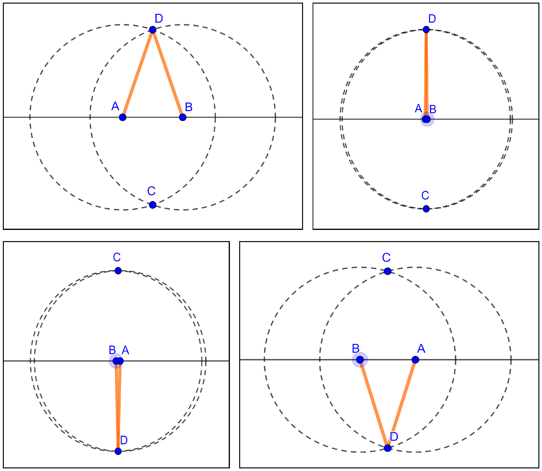
4.1.2. The Problem of Continuity

Another well-known problem arising in the context of DGS is related to the continuity of geometric constructions and the choice of branches in algebraic curves. For a very simple example, let us consider in GeoGebra a linkage with two bars and three vertices A, B and D as shown in Figure 12. The vertex A is fixed at the origin, and the vertex B can move along the horizontal axis y = 0 . The bars have length 1. If the construction is made by the most natural construction (setting D as an intersection point of unit circles centered at A and B), and we slide B along the X-axis, a funny thing happens when B crosses point A from its left side to its right side. The vertex D jumps from the upper half-plane to the lower one, and continuity fails (apart from the fact that D is not defined when A = B ). In a real world bar-and-joint linkage, we would not expect this kind of behavior.
Other example of an unwanted behaviour in DGS linkages is observed in a typical Watt’s linkage construction (see Figure 13), where only one of the two branches that compose the algebraic curve that the point T could describe in a physical model is actually swept in the virtual GeoGebra modelization.
For a comprehensive discussion of the reasons behind these technical issues concerning the continuity of constructions when using a DGS, see [1,22].

4.2. Description of Our Visual Models

We describe here our proposal for a visual model constructed with the DGS GeoGebra. The choice of this software relies not only on the fact that its 3D view allows for a better modelization of 3-dimensional structures, but also because nowadays, GeoGebra stands as one of the most-used DGS in a diverse range of educational and academic environments. As an initial proposal for setting up an appropriate model for the cube, we established the following list of properties that it should have:
1.
Our model can be positioned in any admissible realization, including degenerate ones, after fixing the position of the observer by determining the vertices O, U and E as described in Section 3.
2.
The model is continuous, and joints and bars behave as expected in a real linkage model.
3.
When selecting a vertex to drag it, it has the maximum geometrically possible degree of freedom, as shown in Table 1.
4.
It is reasonably easy to obtain some distinguished configurations, including degenerate ones such as those described in [23].
Unfortunately, the problems described in previous sections about the intrinsic limitations when working with DGS constructions in a straightforward way are a source of difficulties for obtaining a visual model satisfying, simultaneously, all properties initially aimed at. On the other hand, with the software GeoGebra, some of these obstacles can be overcome by means of the use of scripts (sequences of programming commands that are activated and executed when a point is dragged, significantly altering the behavior assigned by default in the DGS) attached to the objects in geometric constructions. These scripts can modify the behavior of elements under certain circumstances (like degenerate realizations) or even impact the whole construction under specific conditions. This will give us some extra flexibility for designing visual equivalents to the mathematical linkages we discussed in previous sections.
In Section 4.1.1, we pointed out the fact that DGS constructions assign fixed degrees of freedom to their vertices. For the cube C * we are working with, with dimension 6 and whose vertices have been labeled O, U, E, F, A, B, J, D, there is a variety of ways of building it in the GeoGebra 3D view with its available tools (see [24] for an introduction to the 3D graphics view in GeoGebra), and depending on the instructions used and the order in which the vertices are determined, the distribution of these 6 degrees of freedom on the vertices do change (we assume degrees 0, 0 for the vertices with given initial conditions O, U respectively). Henceforth, we will describe a distribution of degrees of freedom on the vertices of the cube by means of the corresponding sequence of degrees O d O U d U E d E F d F A d A B d B J d J D d D , where d P is the degree of freedom assigned to vertex P.
Construction 1. In [25], a cubic linkage is shown with our usual initial conditions for its positioning in R 3 : vertices O, U fixed and vertex E lying on plane z = 0 . In this construction point, A moves freely on the 2-dimensional unit sphere with center O, and J has 3 degrees of freedom. Since E is constrained to move along the horizontal unit circle with center O, it has one degree of freedom. Therefore, the distribution of degrees of freedom corresponds to the sequence O0-U0-E1-F0-A2-B0-J3-D0, and all the positions of the cube (except those that imply the coincidence of two or more vertices) are thus determined by the positions of E, A and J. Indeed, a vertex such as B is built as the intersection of the unit spheres with centers A, U and J. Since this intersection in general contains two points, there are two possibilities for choosing B, and this leads to two isomer realizations with respect to B. The same happens with vertices D and F. This explains the isomer options available in the construction. See Figure 14.
Notice also that some restrictions do apply to the movement of these vertices, due to the fact that the unit length of the edges must be preserved. For instance, since the triplet of points { A , E , J } are adjacent to D, they must lie in the unit sphere with center D, and therefore the circumference that they determine must have a radius not greater than 1. Something similar happens with the triplets { U , E , J } , { U , A , J } and { E , A , J } . The use of scripts in GeoGebra facilitates the implementation of these restrictions on the vertices, so that the resulting models do preserve the properties of the linkage when dragging them on the 3D view.
Construction 2. In [26], a more sophisticated model has been designed, starting from a distribution of degrees of freedom O0-U0-E1-F1-A2-B1-J0-D1 for general positions and allowing degenerate constructions when some vertices coincide. Next, we proceed to describe this model in more detail. See Figure 15.
Again, following our usual initial restrictions we have fixed the points O and U. Additionally, the point E describes its path in the z = 0 plane. As in the previous model, point A can move freely on a unit sphere centered at O independently of point E. Thus, the positions of E and A determine the circular paths along which we can attach the vertices F, B and D by means of the GeoGebra command Point(<object>). On the other hand, vertices F, B and D determine only two possible positions for the vertex J, giving rise to two isomer realizations (with respect to J) that can be chosen by marking a checkbox.
One can also make some vertices coincide. These degenerate realizations do change the distribution of degrees of freedom thanks to the use of GeoGebra scripting; in order to easily detect the degrees of freedom that vertices acquire in these particular configurations we have used the following color code:
  • Black: Fixed vertices.
  • Grey: Vertices with 0 degrees of freedom.
  • Blue: Vertices with 1 degree of freedom.
  • Green: Vertices with 2 degrees of freedom.
For instance, by activating the F = O and B = O checkboxes, point J acquires 1 degree of freedom and changes its color to blue. If we also activate the checkbox D = O , vertex D loses its freedom, but point J acquires another degree of freedom, changing its color to green. It is interesting to see here that, whichever configuration is chosen, we can see that the cube never exceeds the 6 internal degrees of freedom that correspond to our algebraically proved fact that the dimension of the linkage V 3 ( C * ) is 6.
Finally, the checkbox J = O activates the particular case in which two opposite vertices of the cube coincide. Note that since, in addition to O, vertex U is also fixed, the vertex E can be no farther than 3 from U. The same happens to vertex A with respect to vertices U and E. These excluded zones for E and A are represented in the construction in the form of shaded spherical caps.

4.3. Related Constructions in Geogebra

During the development of this work, a variety of constructions made in GeoGebra were designed to address different aspects concerning the visualization of linkages in a DGS environment. These constructions have been included in the GeoGebra book [27], and some of them have already been referenced along this work. This broad collection of applets, which constitutes a showcase of different techniques to build linkages in GeoGebra, has been divided into the following sections:
Planar linkages: 
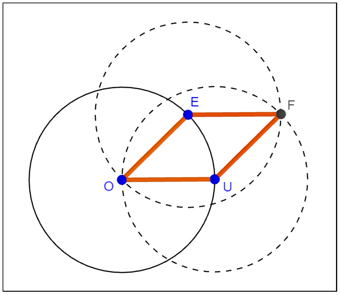
This section describes the fundamentals of planar linkages construction, especially the rhombus (4-bar linkage), as it is the simplest closed and flexible planar configuration available. The intrinsic problems that appear with the use of DGS and are commented on in Section 4.1 are also introduced. Finally, examples of the use of scripts are shown to try to solve them, such as the one that enables the transmission of movement between vertices—what we call the dragging effect—in contrast with traditional geometric constructions in DGS.
Other planar linkages: 
Although the main objective of this GeoGebra book is the study of the structure of the cubic linkage, which corresponds to a graph without one-degree vertices, we considered also chains with either free or fixed extremes (partly because of their interest in connection with applications such as simulations of robotic arms), improving their modeling thanks to the dragging effect mentioned above. In this section, we can see some simple planar examples.
3D linkages: 
This section serves as an introduction to the study of the articulated cube. It shows, in simpler structures, some examples of the problems that will appear in the construction of the cube, such as visualizing certain linkages to decide on their rigidity (as in [28]) or the sudden changes in degrees of freedom mentioned in Example 3.
Articulated cube: 
This is the main section of the GeoGebra book. In addition to constructions 1 and 2 in Section 4.2, we can observe the cube with 6 added bars as described in Section 3.3, with all its 64 possible realizations obtained by means of six parametrized variables. In the opposite direction, a cube is also shown in which no constraints are imposed on its vertices apart from those determined by the fixed length of the bars ([29]). Thanks to the dragging effect already mentioned, which goes beyond the algebraic treatment of linkages developed here, this construction behaves in a very realistic way, offering even an apparent physical behaviour connected to the inner workings of the GeoGebra software.
The interested reader is invited to experiment with this set of constructions and to explore their inner workings by inspecting the GeoGebra scripts attached to some of their constituting elements. Each construction is also accompanied by an explanation of its main characteristics.

4.4. Conclusions and Future Work

Throughout this work, we have addressed some open questions that (at least to our knowledge) first appeared in the last section of [10] and which will help us to summarize our contributions by quoting them and updating their current status:
(i)
“Yet, we have to report that some jumps occur between isomer positions, near singular placements. For instance, when a = 270 , the parallelogram A O B U collapses. In view of the large bibliography on the continuity problem for dynamic geometry, it seems a non-trivial task to model a cube avoiding, if possible at all, such behavior.”
Even though we did not completely solve the continuity problem for linkages, which constitutes an intrinsic difficulty in DGS geometric constructions, through the use of GeoGebra scripts, we have been able to simulate continuity in some of them (see, for example, [29]), although in the process we have lost some of the cleanliness of more formal, purely geometric constructions.
(ii)
“We remark that the cube we have modeled has six internal degrees of freedom, one for each free parameter we have introduced. But its distribution has not been homogeneous. For instance, the final vertex has been constructed without any degrees of freedom, by imposing some constraints: being simultaneously in a sphere and in two planes perpendicular to some diagonals. This difficulty to make a model where all semi-free vertices behave homogeneously is apparently similar to the planar parallelogram case, but now we cannot conclude that it is impossible to make such a construction, since, after fixing O and U we still have six vertices and six degrees of freedom. It is probably a consequence of our approach and not an intrinsic characteristic.”
With respect to the dimension of the cube and the possible degrees of freedom for its vertices, we have completely solved the associated algebraic problem in Section 3, and with respect to distributing homogeneusly the six available degrees of freedom among six vertices of the cube, we have found a construction (see [30]) that achieves this, although without keeping fixed the adjacent vertices O and U.
(iii)
“Could you fix (say, by pasting some rigid plates) one, two,…facets in the cube and still have some flexibility on the cube? How many internal degrees of freedom will remain?"
Some examples of adding bars to limit the flexibility of the cube and the corresponding algebraic discussion have been shown in Section 3.3.
(iv)
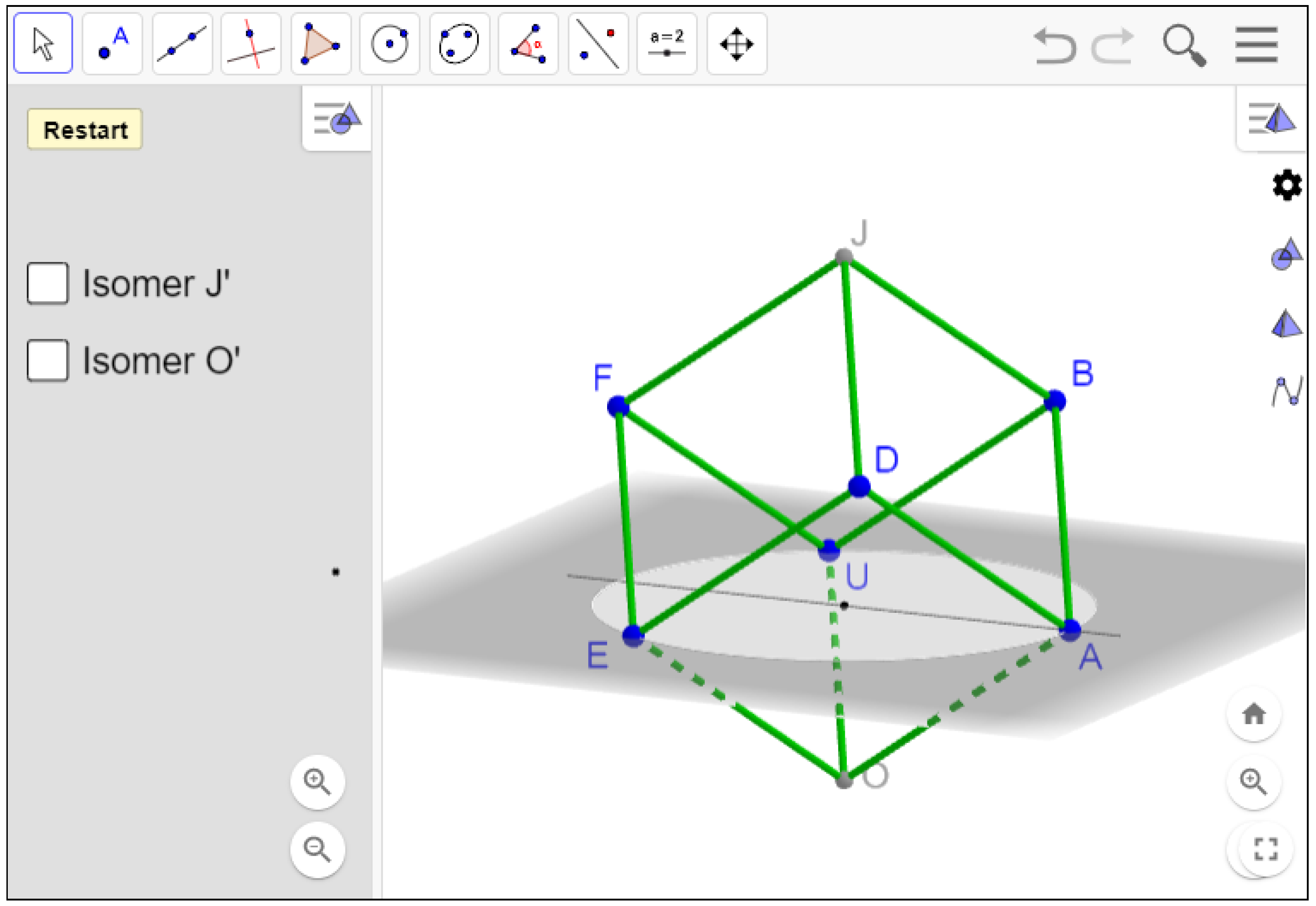
“For a planar parallelogram, one can feel the one-degree of freedom by checking that once you fix one semi-free vertex, the whole parallelogram gets fixed. The same applies for the spatial parallelogram. You have to fix, one after another, the two semi-free vertices. For the cube, how can you feel its six degrees of freedom? Can you fix five semi-free vertices and still move the cube?"
Construction [30] (see also Figure 16) shows an example of a semi-free linkage for the cube where the six degrees of freedom of its internal configurations have been evenly distributed among six of its vertices (U, A, E, B, D and F), leaving two of them (O and J) with 0 degrees of freedom. Notice that, in non-degenerate configurations, dragging any of the vertices B, D or F will leave fixed all the other five vertices with one degree of freedom. This answers (at least partially) in the affirmative the question above.
In comparison to the simplicity of the outcome of that previous approach, we consider that in the current work, we have made contributions in order to gain a better understanding of the cubic linkage, obtaining this time the realization of more sophisticated 3D visualizations in GeoGebra that represent, in our opinion, a step forward to achieve realistic—but symbolic geometry-driven—models of complex linkages in DGS software. Even though we still face pending issues regarding the construction of continuous models that behave, in some sense, closer to linkages in a real world setting, we consider that we have gained a deeper, mathematically well-founded insight concerning diverse aspects such as the algebraic dimension of the cube, the possible distributions of degrees of freedom among its vertices, and the translation of this information into reliable 3D visualizations.
In the near future, we plan to design better DGS applets for this family of dynamic structures, which will look and behave even more like some physical models that can be built with materials as simple as just a few straws and strings (see, for instance, the ingenious devices in [23,31], conceived for their use in a school environment).

Author Contributions

Writing—original draft, T.R., R.L.-L., L.F.T. and C.U.; Writing—review & editing, T.R., R.L.-L., L.F.T. and C.U. All authors have read and agreed to the published version of the manuscript.

Funding

The first and third authors were partially supported by a grant PID2020-113192GB-I00 (Mathematical Visualization: Foundations, Algorithms and Applications) from the Spanish MICINN.

Institutional Review Board Statement

Not applicable.

Informed Consent Statement

Not applicable.

Data Availability Statement

Not applicable.

Acknowledgments

The authors thank Anna M. Bigatti, Robert Corless and Gert-Martin Greuel for their help trying to determine the dimension of the cubic linkage through the use of diverse computer algebra systems.

Conflicts of Interest

The authors declare no conflict of interest.

Abbreviations

The following abbreviations are used in this manuscript:
DGSDynamic geometry software
CASComputer algebra system

References

  1. Kortenkamp, U. Foundations of Dynamic Geometry. Ph.D. Thesis, Swiss Federal Institute of Technology Zurich, Zurich, Switzerland, 1999. [Google Scholar]
  2. Gao, X.S. Automated Geometry Diagram Construction and Engineering Geometry. In Lecture Notes in Artificial Intelligence; Gao, X.S., Wang, D., Yang, L., Eds.; Springer: Berlin/Heidelberg, Germany, 1999; Volume 1669, pp. 232–257. [Google Scholar]
  3. Abanades, M.; Botana, F.; Montes, A. and Recio, T. An algebraic taxonomy for locus computation in dynamic geometry. Comput. Aided Des. 2014, 56, 22–33. [Google Scholar] [CrossRef]
  4. De Graeve, R.; Parisse, B. Giac/Xcas (v. 1.7.0, 2021). Available online: https://www-fourier.ujf-grenoble.fr/~parisse/giac.html (accessed on 29 July 2021).
  5. Kovács, Z.; Parisse, B. Giac and GeoGebra—Improved Gröbner Basis Computations. In Computer Algebra and Polynomials; Gutiérrez, J., Schicho, J., Weimann, M., Eds.; Lecture Notes in Computer Science; Springer: Berlin/Heidelberg, Germany, 2015; pp. 126–138. [Google Scholar]
  6. Polo-Blanco, I. Theory and History of Geometric Models. Ph.D. Thesis, University of Groningen, Groningen, The Netherlands, 2007. [Google Scholar]
  7. Imaginary. Available online: https://www.imaginary.org/ (accessed on 26 February 2022).
  8. Connelly, R.; Demaine, E.D. Geometry and Topology of Polygonal Linkages. In Handbook of Discrete and Computational Geometry, 3rd ed.; Goodman, J.E., O’Rourke, J., Tóth, C.D., Eds.; Chapman and Hall/CRC: New York, NY, USA, 2017. [Google Scholar]
  9. Jordan, D.; Steiner, M. Configuration Spaces of Mechanical Linkages. Discret. Comput. Geom. 1999, 22, 297–315. [Google Scholar] [CrossRef] [Green Version]
  10. Arranz, J.M.; Losada, R.; Mora, J.A.; Recio, T.; Sada, M. Modeling the cube using GeoGebra. In Model-Centered Learning: Pathways to Mathematical Understanding Using GeoGebra; Bu, L., Schoen, R., Eds.; Sense Publishers: Rotterdam, The Netherlands, 2011; pp. 119–131. [Google Scholar]
  11. Bartolini Bussi, M.G.; Taimina, D.; Isoda, M. Concrete models and dynamic instruments as early technology tools in classrooms at the dawn of ICMI: From Felix Klein to present applications in mathematics classrooms in different parts of the world. ZDM Math. Educ. 2009, 42, 19–31. [Google Scholar] [CrossRef]
  12. Sidman, J.; St. John, A. The rigidity of frameworks: Theory and applications. Not. Ams 2017, 67, 973–979. [Google Scholar] [CrossRef]
  13. Recio, T.J.; González-López, M.J. Formal Determination of Polynomial Consequences of Real Orthogonal Matrices. In Recent Advances in Real Algebraic Geometry and Quadratic Forms: Proceedings of the RAGSQUAD Year, Berkeley, 1990–1991; Jacob, W.B., Lam, T.W., Robson, R.O., Eds.; AMS: Providence, RI, USA, 1994. [Google Scholar]
  14. Roth, B. Rigid and flexible frameworks. Amer. Math. Monthly 1981, 88, 6–21. [Google Scholar] [CrossRef]
  15. Connelly, R. Rigidity. In Handbook of Convex Geometry, Vol. A.; Gruber, P.M., Wills, J.M., Eds.; Elsevier: Amsterdam, The Netherlands, 1993. [Google Scholar]
  16. Asimow, L.; Roth, B. The rigidity of graphs. Trans. Amer. Math. Soc. 1978, 245, 279–289. [Google Scholar] [CrossRef]
  17. Asimow, L.; Roth, B. The rigidity of graphs, II. J. Math. Anal. Appl. 1979, 68, 171–190. [Google Scholar] [CrossRef]
  18. Blanc, D.; Shvalb, N. Configuration spaces of spatial linkages: Taking collisions into account. Bull. Korean Math. Soc. 2017, 54, 2183–2210. [Google Scholar] [CrossRef]
  19. Brown, C.W.; Kovács, Z.; Recio, T.; Vajda, R.; Vélez, M.P. Is computer algebra ready for conjecturing and proving geometric inequalities in the classroom? In Proceedings of the 26th Conference on Applications of Computer Algebra, Book of Abstracts, Virtual. 23–27 July 2021. [Google Scholar]
  20. Intersection of Two Spheres. Available online: https://www.geogebra.org/m/h3gbmymu#material/jcyqnmpb (accessed on 5 May 2022).
  21. Parametrized Rigid Cube. Available online: https://www.geogebra.org/m/h3gbmymu#material/ycc5txth (accessed on 10 May 2022).
  22. Kortenkamp, U.H.; Richter-Gebert, J. Complexity issues in Dynamic Geometry. In Foundations of Computational Mathematics. Proceedings of SMALEFEST 2000, Hong Kong, China, 13–17 July 2000; Cucker, F., Rojas, J.M., Eds.; LNAI, 2061; World Scientific: Singapore, 2002; pp. 355–404. [Google Scholar]
  23. Teixidor Cadena, E. Pajifiguri: Un material manipulativo y cuento interactivo. Números Revista de Didáctica de las Matemáticas 2010, 74, 75–92. [Google Scholar]
  24. 3D Graphics View. Available online: https://wiki.geogebra.org/en/3D_Graphics_View (accessed on 1 May 2022).
  25. Articulated Cube (I). Available online: https://www.geogebra.org/m/h3gbmymu#material/txqqrqst (accessed on 8 May 2022).
  26. Articulated Cube (II). Available online: https://www.geogebra.org/m/h3gbmymu#material/tcsy4jut (accessed on 8 May 2022).
  27. Linkages. Available online: https://www.geogebra.org/m/h3gbmymu (accessed on 10 May 2022).
  28. Articulated Prism. Available online: https://www.geogebra.org/m/h3gbmymu#material/qqhj2raa (accessed on 10 May 2022).
  29. Free Articulated Cube. Available online: https://www.geogebra.org/m/h3gbmymu#material/zeagkrck (accessed on 8 May 2022).
  30. Distributing Degrees of Freedom. Available online: https://www.geogebra.org/m/h3gbmymu#material/sff2cs29 (accessed on 10 May 2022).
  31. Teixidor Cadenas, E. 3D, 2D, 1D. Números Revista de Didáctica de las Matemáticas 2016, 92, 93–103. [Google Scholar]
Figure 1. A linkage with 5 bars and 5 joints.
Mathematics 10 02550 g001
Figure 2. Two non-congruent realizations of a linkage with 5 vertices and 5 unit-length edges.
Mathematics 10 02550 g002
Figure 3. A triangular free linkage in the plane.
Mathematics 10 02550 g003
Figure 4. A linkage with different real/complex behaviours.
Mathematics 10 02550 g004
Figure 5. The cubic linkage C.
Mathematics 10 02550 g005
Figure 6. A linkage whose dimension grows in degenerate cases.
Mathematics 10 02550 g006
Figure 7. A finitely rigid plane linkage.
Mathematics 10 02550 g007
Figure 8. Realizations for V 2 ( P D ( i ) ) for i = 1 , 2 , 3 , 4 .
Mathematics 10 02550 g008
Figure 9. Adding bars to the cube to make it rigid.
Mathematics 10 02550 g009
Figure 10. Is this a rigid cube?
Mathematics 10 02550 g010
Figure 11. A square linkage.
Mathematics 10 02550 g011
Figure 12. Continuity problems in DGS linkages.
Mathematics 10 02550 g012
Figure 13. The Watt’s linkage, showing in green the swept branch of the geometric locus.
Mathematics 10 02550 g013
Figure 14. A GeoGebra cube with degrees of freedom O0-U0-E1-F0-A2-B0-J3-D0.
Mathematics 10 02550 g014
Figure 15. A GeoGebra cube with degrees of freedom O0-U0-E1-F1-A2-B1-J0-D1 with degenerate cases.
Mathematics 10 02550 g015
Figure 16. A uniform distribution of six degrees of freedom among six vertices.
Mathematics 10 02550 g016
Table 1. Degrees of freedom of the vertices of the cube.
VertexVariablesRestrictionsDegrees of Freedom
O 0
U 0
A { A x , A y , A z } B = A + U 2
F = E + U
J = D + U
B { B x , B y , B z } B = A + U 2
F = E + U
J = D + U
D { D x , D y , D z } B = A + U 3
F = E + U
J = D + U
E { E x , E y } A = O + Z 1
B = U + Z
J = F + Z
D = E + Z
F { F x , F y , F z } A = O + Z 2
B = U + Z
J = F + Z
D = E + Z
J { J x , J y , J z } B = A + U 3
F = E + U
J = D + U
Table 2. Representatives of non-congruent realizations of the rigid cube C R .
( A x , A y , A z ) ( B x , B y , B z ) ( D x , D y , D z ) ( E x , E y , E z ) ( F x , F y , F z ) ( J x , J y , J z )
( 0 , 0 , 1 ) ( 0 , 1 , 1 ) ( 1 , 0 , 1 ) ( 1 , 0 , 0 ) ( 1 , 1 , 0 ) ( 1 , 1 , 1 )
( 0 , 0 , 1 ) ( 2 3 , 1 3 , 1 3 ) ( 1 , 0 , 1 ) ( 1 , 0 , 0 ) ( 1 , 1 , 0 ) ( 1 , 1 , 1 )
( 0 , 0 , 1 ) ( 0 , 1 , 1 ) ( 1 3 , 2 3 , 1 3 ) ( 1 , 0 , 0 ) ( 1 , 1 , 0 ) ( 1 , 1 , 1 )
( 0 , 0 , 1 ) ( 0 , 1 , 1 ) ( 1 , 0 , 1 ) ( 1 , 0 , 0 ) ( 1 3 , 1 3 , 2 3 ) ( 1 , 1 , 1 )
( 0 , 0 , 1 ) ( 2 3 , 1 3 , 1 3 ) ( 1 3 , 2 3 , 1 3 ) ( 1 , 0 , 0 ) ( 1 , 1 , 0 ) ( 1 , 1 , 1 )
( 0 , 0 , 1 ) ( 0 , 1 , 1 ) ( 1 3 , 2 3 , 1 3 ) ( 1 , 0 , 0 ) ( 1 3 , 1 3 , 2 3 ) ( 1 , 1 , 1 )
( 0 , 0 , 1 ) ( 2 3 , 1 3 , 1 3 ) ( 1 , 0 , 1 ) ( 1 , 0 , 0 ) ( 1 3 , 1 3 , 2 3 ) ( 1 , 1 , 1 )
( 0 , 0 , 1 ) ( 2 3 , 1 3 , 1 3 ) ( 1 3 , 2 3 , 1 3 ) ( 1 , 0 , 0 ) ( 1 3 , 1 3 , 2 3 ) ( 1 , 1 , 1 )
( 0 , 0 , 1 ) ( 2 3 , 1 3 , 1 3 ) ( 1 3 , 2 3 , 1 3 ) ( 1 , 0 , 0 ) ( 1 3 , 1 3 , 2 3 ) ( 1 3 , 1 3 , 1 3 )
( 0 , 0 , 1 ) ( 4 9 , 1 9 , 1 9 ) ( 1 3 , 2 3 , 1 3 ) ( 1 , 0 , 0 ) ( 1 3 , 1 3 , 2 3 ) ( 1 3 , 1 3 , 1 3 )
( 0 , 0 , 1 ) ( 2 3 , 1 3 , 1 3 ) ( 1 9 , 4 9 , 1 9 ) ( 1 , 0 , 0 ) ( 1 3 , 1 3 , 2 3 ) ( 1 3 , 1 3 , 1 3 )
( 0 , 0 , 1 ) ( 2 3 , 1 3 , 1 3 ) ( 1 3 , 2 3 , 1 3 ) ( 1 , 0 , 0 ) ( 1 9 , 1 9 , 4 9 ) ( 1 3 , 1 3 , 1 3 )
( 0 , 0 , 1 ) ( 4 9 , 1 9 , 1 9 ) ( 1 3 , 2 3 , 1 3 ) ( 1 , 0 , 0 ) ( 1 9 , 1 9 , 4 9 ) ( 1 3 , 1 3 , 1 3 )
( 0 , 0 , 1 ) ( 4 9 , 1 9 , 1 9 ) ( 1 9 , 4 9 , 1 9 ) ( 1 , 0 , 0 ) ( 1 3 , 1 3 , 2 3 ) ( 1 3 , 1 3 , 1 3 )
( 0 , 0 , 1 ) ( 2 3 , 1 3 , 1 3 ) ( 1 9 , 4 9 , 1 9 ) ( 1 , 0 , 0 ) ( 1 9 , 1 9 , 4 9 ) ( 1 3 , 1 3 , 1 3 )
( 0 , 0 , 1 ) ( 4 9 , 1 9 , 1 9 ) ( 1 9 , 4 9 , 1 9 ) ( 1 , 0 , 0 ) ( 1 9 , 1 9 , 4 9 ) ( 1 3 , 1 3 , 1 3 )
Publisher’s Note: MDPI stays neutral with regard to jurisdictional claims in published maps and institutional affiliations.

