Abstract
Mine extraction planning has a far-reaching impact on the production management and overall economic efficiency of the mining enterprise. The traditional method of preparing underground mine production planning is complicated and tedious, and reaching the optimum calculation results is difficult. Firstly, the theory and method of multi-objective optimization are used to establish a multi-objective planning model with the objective of the best economic efficiency, grade, and ore quantity, taking into account the constraints of ore grade fluctuation, ore output from the mine, production capacity of mining enterprises, and mineral resources utilization. Second, an improved particle swarm algorithm is applied to solve the model, a nonlinear dynamic decreasing weight strategy is proposed for the inertia weights, the variation probability of each generation of particles is dynamically adjusted by the aggregation degree, and this variation probability is used to perform a mixed Gaussian and Cauchy mutation for the global optimal position and an adaptive wavelet variation for the worst individual optimal position. This improved strategy can greatly increase the diversity of the population, improve the global convergence speed of the algorithm, and avoid the premature convergence of the solution. Finally, taking a large polymetallic underground mine in China as a case, the example calculation proves that the algorithm solution result is 10.98% higher than the mine plan index in terms of ore volume and 41.88% higher in terms of economic efficiency, the algorithm solution speed is 29.25% higher, and the model and optimization algorithm meet the requirements of a mining industry extraction production plan, which can effectively optimize the mine’s extraction plan and provide a basis for mine operation decisions.
MSC:
90C29
1. Introduction
The preparation of the extraction plan, as a basic link in the production operation of a mining enterprise, is one of the most critical tasks in the production decision of a mine, and the rationality of the plan preparation directly affects the efficiency of the subsequent production links and the overall economic efficiency of the mining enterprise [1,2,3]. The traditional manual preparation method is not only time-consuming and intensive but also has poor accuracy and is difficult to modify. The reason for this is mainly the complex underground mine conditions during the preparation of the plan, which requires comprehensive consideration of the spatial and temporal constraints between the production processes and the mines and their continuity. Therefore, how to develop the underground mine production plan quickly and accurately has been an urgent problem to be solved.
With the continuous advancement of computer technology and operations research theory, many researchers have started to try to use the powerful simulation computing power of computers to simulate the mine production process, so as to continuously optimize the mine extraction plan [4,5]. Several researchers recognize that integer programming can solve discrete production scheduling decision problems in the mining industry [6,7]. Many studies on mine production planning related to integer programming theory were subsequently carried out [3,8,9,10,11,12]. Dimitrakopoulos and Ramazan [13] developed an optimization framework for stochastic mine production scheduling considering mine uncertainties based on an ore body model and an integer planning approach. Weintraub et al. [14] developed a large, aggregated integer planning model (MIP) based on cluster analysis for mine planning at CODELCO, a national copper mine in Chile, through which data information of all CODELCO mines can be obtained to optimize the mine extraction planning. Newman et al. [15] developed a mixed integer planning model for underground mining operations in Kiruna mine, Sweden. This optimization model identifies an operationally feasible recovery sequence that minimizes deviations from the planned production quantities. Terblanche and Bley [16] used a mixed integer planning approach to construct a theoretical model applicable to the optimization of extraction production plans for open pit and underground mines but did not verify the feasibility of the model. Nehring et al. [17] proposed an improved modified model formulation for the classical model of long-term mine planning, assigning different human resources and equipment to each mining area. In the classical model, only one binary variable is assigned to each activity in each mining area, whereas the improved model assigns one binary variable to all activities under a more stringent assumption.
Although there are more existing studies on mathematical planning methods, most of these models achieve the solution of mine production planning with a single economic indicator; however, since mine extraction production planning is a complex system of engineering, it is difficult to highlight the production plan preparation and optimization effect by considering only a single economic indicator [18]. In order to overcome these difficulties, researchers have used a variety of computational intelligence methods to solve multi-objective prediction and optimization problems, and heuristic algorithms are effective methods to improve the solution speed and avoid involving local optimal solutions, while having unique advantages for multi-objective optimization problems (MOP). Little and Topal [19] investigated the methodology of whole life of mine (LOM) production planning generated using a simulated annealing technique and stochastic simulation representation of the ore body with the objective of maximizing the net present value (NPV) of the mine. Hou et al. [20] addressed the production planning for the next three years of the mine using an artificial bee colony optimization algorithm. Otto and Bonnaire [21] developed a “Greedy randomized adaptive search” program to help solve models for copper mining development and improve the speed of solution. O’Sullivan and Newman [22] proposed an optimization heuristic algorithm to set a complex set of constraints based on an optimization algorithm in a mining operation model for an underground lead–zinc mine in Ireland. Wang et al. [23] proposed a multi-objective optimization model formulation by taking the grade of mined and processed ore as the main constraint, maximizing mining returns and efficient use of natural resources as the objective function, and used a genetic algorithm to find the optimal solution to the multi-objective optimization problem. Nesbitt et al. [24] considered the uncertainty faced in the economic value of minerals faced by mines with long operating cycles. For a hard rock mine, the method of creating a stochastic integer program helps the mine to customize a mining schedule with a high degree of feasibility.
However, the use of traditional heuristic algorithms in the preparation of mining industry extraction production plans leads to slow solution speed and reduced global convergence performance, which brings many difficulties to the preparation and optimization effect of the actual production operation plan in real time and has a profound impact on the production management and economic efficiency of the enterprise. Therefore, in order to solve these problems, which are due to the complexity of multi-metal mine production planning, and since it is difficult to achieve the optimal results by traditional methods, this paper takes the best economic efficiency, grade, and ore volume as the goal and integrates constraints such as ore grade fluctuation, ore output of mining sites, mine production capacity, and mineral resource utilization. A production planning model is established, and the model is optimally solved by an improved particle swarm optimization (PSO) algorithm with nonlinear inertia weights and adaptive mutation probability (NAMPSO) in the context of an engineering example to improve the model’s solving speed and increase the global convergence performance of the algorithm, thereby verifying the feasibility of the model solution method.
2. Balanced Mining Plan Model
2.1. Model Analysis
There are many factors that need to be considered comprehensively in the preparation of an underground mine extraction plan, and by analyzing the current situation faced by underground mining and the existing mining technology conditions [25,26,27,28,29,30], the main factors that need to be considered in the process of extraction plan preparation are shown in Figure 1.
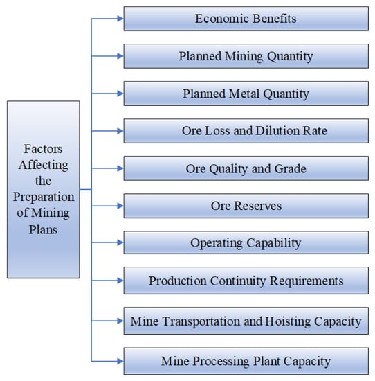
Figure 1.
Factors affecting the preparation of the mining plan.
- (1)
- Economic efficiency: when mining in the market economy, the first factor to consider is the economic factors, that is, to ensure that the mining enterprise can obtain a better economic benefit.
- (2)
- The planned quantity of mining: for mining enterprises to carry out normal operations, mining plans must be able to ensure the mine’s subsequent production of ore demand.
- (3)
- Planned metal quantity: for mines with metal quantity as the production target, the quantity of ore mined should be guaranteed to meet the requirements of metal quantity for production and processing.
- (4)
- Ore loss and dilution ratios: in the process of balanced mining in underground metal mines, ore loss and dilution ratios must be controlled in order to ensure the maximization of the comprehensive benefits of the enterprise and the maximization of resource recovery and utilization.
- (5)
- Ore quality and grade: due to the variability of mineral resources endowment, there are differences in quality and grade of ore per mining site; therefore, the development of the extraction plan needs to take full account of such differences and achieve the requirements of the extracted ore in terms of quality and grade through reasonable planning.
- (6)
- Ore reserves: to achieve balanced mining, the development of the extraction plan must take into account the limits of the ore reserve of each mineral deposit and mine excavation.
- (7)
- Operating capability: mining enterprises need to have a full understanding of the existing production technology conditions of the mine, production equipment, and the ability and quality of operators when formulating the extraction plan.
- (8)
- Production continuity requirements: once the mine is established, it must ensure that production activities can be carried out continuously and steadily; therefore, the mine’s mining plan must consider the ore reserves of the mineral deposit, cutting, retrieval, and preparation for mining to ensure that the mine production activities can be carried out continuously and steadily.
- (9)
- Mine transportation and hoisting capacity: Most of the waste rock and all the ore produced by underground metal mines rely on haulage and hoisting equipment to transport and hoist. The production capacity of the mine must be matched with the transport and hoisting capacity of the mine.
- (10)
- Mine processing plant capacity: in order to avoid the long-term backlog of mined ore, resulting in increased mining production costs or affecting underground mining operations, the total output of ore during the planning period is generally required to be on par with the processing capacity of the plant.
In principle, each underground metal mine plan should consider all the factors in Figure 1, but in practice some factors can be combined and simplified according to the actual situation of the specific mine. For example, only one of the planned mining quantities and planned metal quantity are required, and only the smaller of the mine transport and hoisting capacity and mine processing plant capacity should be considered. At the same time, it is possible to add other influencing factors.
The process of preparing an extraction plan based on balanced mining is essentially a process of seeking an extraction solution that meets the requirements of various stakeholders in the process of comprehensive coordination of various constraints. Therefore, with the help of the objective optimization method in operations research theory, the complex extraction planning can be transformed into an MOP problem model by converting various restrictions into constraints and the final objective into an objective function, thus turning the complex programming process into a mathematical optimization problem.
2.2. Model Building
2.2.1. Model Assumptions
This modeling is carried out based on the following three basic assumptions:
- (1)
- The mining method assumed for the model is room-and-pillar mining. The mine development system has been completed before the preparation of the mining plan, and the mining plan constructed in this paper mainly includes the output of each mineral deposit and the mining cut of each block during the planning period.
- (2)
- The ore reserves, the grade of each metallic element in the ore, and the content of contaminants in each mineral deposit (including the mined room, the mined pillar, the mined and cut room, the mined and cut pillar, and the complete block that has not yet been mined) have all been proven.
- (3)
- The planned mineral deposits should be capable of simultaneous mining operations.
2.2.2. Model Parameters Definition
This model parameters are defined at the end of the paper.
2.2.3. Objective Functions
Equation (1) indicates the maximization of corporate revenue: from the perspective of corporate profitability, one of the purposes of mining enterprises conducting extractive operations is to obtain economic benefits, so the maximization of corporate revenue is one of the main objectives of the preparation of the extraction plan.
Equation (2) indicates the grade optimization: from the perspective of mineral processing, due to the variability of mineral resource endowment, the development of the extraction plan needs to take full account of such differences to achieve the minimum fluctuations in the average grade of the extracted ore.
Equation (3) indicates the ore production maximization: the more ore extracted during the planning period, the higher the production efficiency and the better the mining operation.
2.2.4. Constraints
After establishing the target of the extraction plan, it is necessary to transform each restriction into the constraint of the target function. Combined with the actual underground mining, the constraints are mainly the following six kinds.
Equation (4) indicates the metal quantity constraint: the actual quantity of metal produced cannot be lower than the minimum amount of metal required during the planning period.
Equation (5) indicates the ore reserve constraint: the ore reserves of each mine room and pillar, as well as the ore reserves of the mining preparation works, are limited and cannot be exceeded.
Equation (6) indicates the production capacity constraints: the development of extraction plans needs to consider the existing technical conditions of the mine’s production and production equipment, etc., and cannot exceed the maximum production capacity.
Equation (7) indicates the production continuity constraints: once the mine is fully operational, it must ensure that production activities can be carried out continuously and steadily; therefore, the mine’s mining plan must be prepared to consider mining preparation blocks. Back mining blocks in the ore reserves can be articulated reasonably as the general requirements of the planned period for mining preparation blocks, and the ore reserves are not less than the planned period for back mining of ore to ensure that the mine production activities can be carried out continuously and steadily.
Equation (8) indicates the mine hoisting capacity constraint: the mining capacity cannot exceed the maximum hoisting capacity of equipment during the planning period.
Equation (9) represents the variable non-negative constraint: recovery of ore quantity in all mine rooms and pillar and mining preparation block quantity are non-negative quantities that are greater than or equal to zero.
2.3. Optimized Solution
The optimal solution to the objective is the optimal operation plan for the planning period. However, due to the large number of decision variables, it is difficult to find the optimal solution by manual calculation. In order to solve the above MOP problem, this paper does not use the traditional single-objective processing methods, such as weight coefficient summation or objective constraint, but finds a set of feasible solutions based on the Pareto optimal solution set in order to provide more decision options for the decision maker. Therefore, it is necessary to find an appropriate algorithm and then solve the problem with the powerful computing facilities. In this paper, an improved particle swarm algorithm is adopted to solve the above MOP problem [31].
3. Materials and Methods
3.1. Basic Particle Swarm Optimization Algorithm
The particle swarm algorithm was proposed by Kennedy, an American psychologist, and Dr. Eberhart, an electrical engineer, in 1995 [32]. This algorithm is used to guide the updating of the velocity and position of the next generation of particles by the individual optimal position and the global optimal position of the particles in the population, so that the particles always move toward the individual optimal position and the global optimal position and finally converge to the global optimal position [33,34].
In the M-dimensional search space, there exists a population consisting of N particles, where , ; the velocity and position components of the i particle at the t iteration in the j dimension are and , respectively; denotes the optimal position component of the particle; denotes the optimal position component of the population; w is the inertia weight coefficient; is the learning factor; is a random number obeying uniform distribution within (0, 1) [35].
The velocity and position update of the basic particle swarm algorithm are as indicated by Equations (10) and (11) [36].
3.2. Optimization Strategies
3.2.1. Nonlinear Dynamic Decreasing Inertia Weighting Strategy
The inertia weight w is one of the important parameters affecting the performance of PSO algorithm. The larger the inertia weight is, the faster the particle swarm moves, the ability to search the local space is reduced, and the ability to detect the global space is enhanced; the smaller the inertia weight is, the lower the speed of the particle moves, the ability to search the local space is enhanced, and the ability to detect the global space is reduced. Therefore, appropriate improvement of inertia weights can improve the performance of the PSO algorithm. For this reason, Shi [37] proposed a linear decreasing particle swarm optimization (LDPSO) algorithm, with the following linear decreasing inertia weight strategy:
where denotes the maximum number of iterations; denotes the current number of iterations; and denote the set maximum inertia weights and minimum inertia weights, respectively. Through several experimental analyses, the authors found that as the number of iterations increases, when , the search performance of the algorithm is greatly improved [38,39].
In this paper, based on the LDPSO algorithm and inspired by the ideas in the literature [39,40,41,42], we propose a nonlinear dynamic decreasing weight strategy particle swarm optimization (NDIWPSO) algorithm in which the inertia weights are set as nonlinear exponential functions, as shown in Equation (13):
where k is the control factor. Compared with LDPSO, when w is close to , the value of w increases, and NDIWPSO is dominated by the first term of Equation (10) during most of the iterations. Then, the ability of the particle to expand the search space is enhanced, and it is more advantageous in searching the global space, while the contraction ability of the particle to the location of the optimal value decreases, and the ability to search the local space is then weakened; when is close to , the value of w decreases and NDIWPSO is dominated by the last two terms of Equation (10) during most of the iterations, and then the particle is more advantageous in searching for the optimal value in the local interval, and the ability to search the global space is weakened. So, the nonlinear exponential function, Equation (13), can coordinate the algorithm to achieve better between the ability of local search and global search.
3.2.2. Dynamic Learning Factor Strategy
In addition to the inertia weights , the learning factors , also need to be improved to make them more suitable for system optimization search.
Equations (14) and (15) are the improvement of the learning factor [42]; as the iterative process proceeds, decreases while increases, and in the early iterative process, the particles are mainly influenced by the individual information, which is beneficial to increase the population diversity. In the later iterative process, the particles are mainly influenced by the population information, which is beneficial to the particles to rapidly approach the global extremes and obtain the optimal solution.
3.2.3. Adaptive Variation Probability and Global Optimal Hybrid Mutation Strategy
In order to increase the diversity of the population, a variation strategy is applied to it based on the previous optimization, which leads the particles to jump out of the local optimal value points and search in a more global space. The specific implementation is as follows.
If , , represent the mean, maximum and minimum values of particle fitness in the generation, respectively, then Equation (16) for the aggregation degree of particles in the generation is as follows.
When the deviation of the fitness of individual particles from the overall average fitness is larger, the diversity of particles is better, and vice versa, the diversity of particles is worse. Therefore, when is larger, the diversity of particles is better, and when is smaller, the diversity of particles is worse. Therefore, the aggregation degree can be used to dynamically adjust the probability of variation of particles in each generation, and let the probability of variation in the generation be , as shown in Equation (17). α is used to regulate how fast the variance probability changes and is a constant that takes values in the range [2,4].
In this paper, a mutation on the optimal position of the particle is used, and if , a mixture of Gaussian (Equation (18)) and Cauchy (Equation (19)) distributions is used to vary the optimal position of the particle. denotes a random one of the global optimal and global suboptimal positions; denotes the global optimal position; is a random number of Gaussian distribution; is a random number of Cauchy distribution.
The pseudo-code for the global optimal hybrid mutation strategy is Mut1 (Algorithm 1).
| Algorithm 1: Mut1. |
| begin |
| if rand < 0.5 |
| else |
| end |
| ); |
| end |
| − 0.5)); |
| ); |
| end |
| end |
3.2.4. Worst Personal-Best Position Adaptive Wavelet Mutation Strategy
In the above hybrid variation strategy, the global optimal and suboptimal extremes are utilized for variation, while the worse individual extremes are not utilized. In fact, in the population, the worse individual extremes have limited guiding effect on the particles; thus, variation on the worse individual extremes is beneficial to accelerate the convergence of the population.
The worst individual optimal adaptive wavelet variation strategy [43] (Mut2):
The worst individual extreme value particle is selected, and the search boundary of the selected particle in the dimension is . is varied according to Equation (21), and in this paper, adaptive wavelet variation is used to improve the worst individual extreme value to speed up the evolution of the population. is the wavelet function value, is the wavelet function, and Morlet wavelet is chosen as the wavelet base in Equations (22)–(24). a is the scale parameter, and more than 99% of the energy of the wavelet function is contained in (−2.5, 2.5), so the range of values of in the formula is the pseudo-random number of (−2.5a, 2.5a) [44]. The wavelet amplitude decreases continuously with the increase of parameter . In order to adjust the wavelet amplitude adaptively, the adaptive parameter a is proposed in this paper, and its expression is Equation (25). k and a0 are positive constants, and this paper sets .
3.3. Algorithm Steps
- Step 1.
- (Initialization): set the current number of iterations , the maximum number of iterations , the population size N, the dimensionality of the search space M, and the initial position and velocity of each particle generated randomly.
- Step 2.
- (Optimal update): the velocity and current position of each particle are updated according to Equations (10), (11) and (13)–(15), and the value of the fitness function is calculated for each particle.
- Step 3.
- (Individual Optimal Update): for each particle , if the current fitness function value is better than the individual historical optimal position , update the individual optimal .
- Step 4.
- (Global Optimal Update): for each particle , if the current fitness function value is better than the global optimal position , the global optimal is updated.
- Step 5.
- Calculate the aggregation degree and the variation probability of the particle population according to Equation (16); if , mutate according to the mutation strategies Mut1 and Mut2 in Section 3.2.3 and Section 3.2.4.
- Step 6.
- Calculate the particle fitness and update and .
- Step 7.
- and return to step 2 until t reaches the set maximum number of iterations and stop.
- Step 8.
- The optimal result is output, and the algorithm is finished.
3.4. Construction of the Fitness Evaluation Function
For the MOP problem model of the extraction plan, this paper uses the evaluation function method to construct the fitness function. Specifically, we set an arbitrary best value and for the objective functions and respectively, and construct the fitness evaluation function of the extraction plan by calculating the difference between each objective function and it and pursuing the minimum of the sum. Equation (26). is the planned quantity of ore to be produced, is the planned economic efficiency of the enterprise during the plan period.
4. Engineering Applications and Results Analysis
4.1. Mine Engineering Overview and Basic Data
In order to verify the effectiveness of the NAMPSO algorithm for industrial mining planning of multi-metal mines, the actual mining production data of a large underground metal mine rich in gold (Au), antimony (Sb), and tungsten (WO3) in Hunan Province, China, are taken as an example, and the numerical model of the mine is shown in Figure 2. In this paper, the annual production task index of this mine and the actual situation of the mine are combined, and the balanced mining extraction plan model established in Section 2 and the NAMPSO algorithm for solving multi-objective optimization problems proposed in Section 3 are applied to optimize the extraction plan of this mine for each quarter and obtain the annual optimal mining plan.
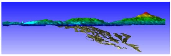
Figure 2.
Digital model of underground multi-metal mine.
The production target of the mining company for this mine in the current year is shown in Table 1.

Table 1.
Production task indicators.
Among them, after the completion of the mining tasks of the previous year, the ore reserves of the mine’s preparation rooms (13) and preparation pillars (8), as well as the part of the works of the excavated blocks (9) that need to be completed in this year, are shown in Table 2.
Table 2.
Parameters of the mine rooms, mine pillars, and excavated blocks.
4.2. Balanced Mining Model Parameters
According to the balanced mining extraction plan model constructed in Section 2.2 of this paper, the parameters involved in the mathematical model of the extraction plan are organized as follows, considering the actual situation of the mine and referring to the production experience of the mine in previous years:
- (1)
- Excavated blocks = 9, Mine pillars = 8, Mine rooms = 13.
- (2)
- Production ore quantity factor for block mining preparation works = 4.2 t/m, Quantity of ore contained in 1 m of mining preparation = 166.7 t/m.
- (3)
- Quantity factor of prepared mining blocks/ during the plan period = 1.
- (4)
- Maximum mining capacity: = 25,000 t, = 25,000 t, = 180 m.
- (5)
- Metal types = 3, Average quarterly ore output = 20,000 t, Maximum underground hoisting capacity quarterly = 35,000 t.
- (6)
- Gold concentrate contains gold price (metal price) = 235,000 Yuan/kg, antimony concentrate contains antimony price (metal price) = 29,700 Yuan/t (antimony concentrate valuation coefficient is 0.6), tungsten concentrate contains tungsten price = 150,000 Yuan/t. The quarterly revenue required by the enterprise can be calculated according to the quarterly metal quantity task as = 22,488,750.
4.3. Algorithm Parameter Setting
For the above engineering example data and the constructed model, the algorithm is applied on the MATLAB platform to solve the plan model optimally. There are 30 parameters of decision variables in this metal mine mining planning model, so the dimension of each particle in the algorithm = 30; the population size of particles = 150, the number of iterations = = 3000; the learning factor varies with the number of iterations ; the ore loss rate of the mining site is considered to be 5%.
4.4. Engineering Example Simulation
Based on the equilibrium mining model and the data in Table 1 and Table 2, the PSO algorithm and the NAMPSO algorithm were applied to find the optimal extraction plan for each quarter of a year, and the iterative convergence process of the model solution was calculated to obtain four quarters, as shown in Figure 3. From the fitness function curves, we can see that the fitness function values of the two algorithms are close to the improved algorithm slightly better, but the convergence speed of the improved PSO algorithm is significantly faster in the first two quarters (PSO converges around the 1550th, 450th, 1400th, and 120th generations, and NAMPSO converges around the 1100th, 250th, 1200th, and 80th generations), the convergence speed is improved by about 29.25%, and the specific results of the balanced extraction plan are shown in Table 3, Table 4 and Table 5.
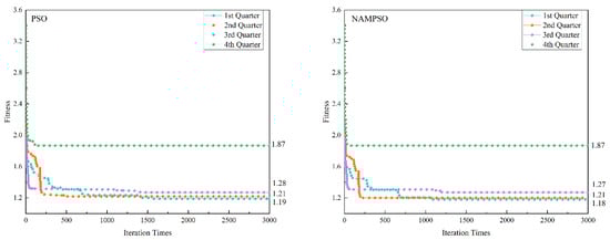
Figure 3.
Convergence curve of the optimal adaptation degree of the mining plan.
Table 3.
Quarterly and annual mining plan.
Table 4.
Quarterly and annual excavation plan.
Table 5.
Extraction plan optimization results by quarter and year.
From the convergence curve in Figure 3, it can be seen that when the NAMPSO algorithm is used to solve the extraction plan, the value of the objective function fluctuates between 3.2 and 1.2 when the number of iterations is between 0 and 500, indicating that the algorithm converges to the global optimal solution slowly at the early stage of iterative computation when the number of particles within the population is high under a certain initial population size and at the late stage of iterative computation, i.e., after 500 iterations, the algorithm starts to converge smoothly and rapidly to the global optimal solution of the objective function. It can also be seen that the NAMPSO algorithm, when solving the production planning model with complex constraints, performs nonlinear dynamic optimization of the inertia weights of the algorithm and introduces an adaptive variational probability strategy to make the particles outside the feasible domain enter the feasible domain quickly, which leads to a slow convergence computation at the early stage of the algorithm search, while the computation speed of the algorithm is faster at the later stage, and it is easy to jump out of the local optimal solution problem.
4.5. Analysis of Results
Combined with the enterprise’s target requirements for the mine’s extraction production, a comparative analysis of the extraction plans given in this paper for each quarter shows that:
- (1)
- As shown in Figure 4, in terms of mining quantity, the actual mining quantity of each quarter and year in the balanced mining plan is slightly higher than the planned mining quantity, which can meet the annual mining quantity target specified by the enterprise. At the same time, the proportion of mining quantity in each quarter is 26%, 25%, 24%, and 25%, respectively, which meets the requirement of balanced mining.
 Figure 4. Convergence curve of the optimal adaptation degree of the mining plan.
 - (2)
- As shown in Figure 5, in terms of the production of gold, antimony, and tungsten, the actual production for each quarter and year in the extraction plan given in this paper is slightly higher or equal to the planned production, which fully meets the annual metal production target set by the enterprise. The percentages of gold production in each quarter are 24%, 23%, 24%, and 29%, respectively; the percentages of antimony production in each quarter are 26%, 24%, 23%, and 27%, respectively; and the percentages of tungsten production in each quarter are 25%, 25%, 25%, and 25%, respectively. From the absolute uniform distribution of tungsten production in each quarter, it can be seen that the algorithm takes the achievement of tungsten production as one of the key conditions when searching for the optimal mining plan, which fully meets the metal content constraint requirement of the model, and because the grade of tungsten is relatively the lowest among the three metals in the ore of each mining site, the value of tungsten is relatively the lowest among the three metals, and the recovery rate of tungsten beneficiation is also the lowest.
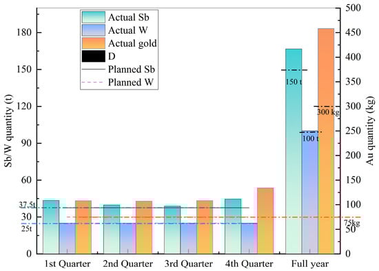 Figure 5. Comparison of actual and planned production of metal quantities.
 - (3)
- As shown in Figure 6, the average grade of gold and tungsten is higher than the planned ore grade, the average grade of gold and tungsten in the ore mined in each quarter is basically balanced, and the average grade of antimony in the ore mined in each quarter is basically the same as the planned grade. Therefore, the mining plan searched by the method of this paper achieves the balance of the ore grade, and the ore grade fluctuation is small.
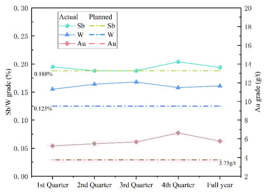 Figure 6. Comparison of actual grade and planned grade of ore mined.
 - (4)
- As shown in Figure 7, in terms of economic benefits, the annual economic benefits of the extraction plan given in this paper increased by 41.88% compared to the planned economic benefits. The actual production of each quarter and year is slightly higher than the planned production, and the production of each metal also meets the requirements, so the economic benefits of each quarter and year are necessarily higher than the planned economic benefits, and the actual benefits of each quarter account for 24%, 23%, 24%, and 29%, respectively, and in general, the economic benefits of each quarter are balanced and stable, which can well fulfill the benefit targets given by the company.
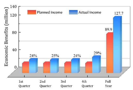 Figure 7. Comparison of actual and planned economic benefits.
 - (5)
- As shown in Figure 8, in terms of mining balance, in order to seek the quarterly quantity of ore production that satisfies each constraint, the quantity of ore mined from each mineral deposit (including the mine room and pillar) varies each quarter, which reflects the equilibrium process of ore matching. Through four quarters of mining, the ore reserves of each mining field are basically depleted, and in actual production the ore reserves of the mining field can be considered as the end of mining when they are below a certain value. After one year of mining, most of the 21 recovery mining fields involved in the plan can be considered as completed. In order to ensure that mine production can be carried out continuously, it is necessary to adhere to the principle of balanced mining and excavation with excavation first. In this paper, the mining plan is formulated mainly through the balance between the recovery quantity and mining preparation quantity to ensure the continuity of production, as shown in Figure 9. This paper contains nine mining preparation fields, each of which has a different footage of excavation in each quarter, and the reason for this is that the quantity of ore production from each mining preparation project also must meet the production constraints. After four quarters of mining preparation work, the nine mining preparation fields are basically finished and can be used as back mining fields for the next year, which can ensure the continuous progress of production work in the next year.
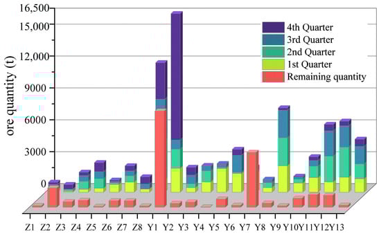 Figure 8. Distribution of ore production and remaining ore in each mining field by quarter.
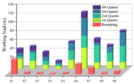 Figure 9. Distribution of excavation works and remaining works in each mining field by quarter.
5. Conclusions
Aiming at the multi-objective optimization problem faced by underground multi-metal mine extraction plans, this paper proposes an improved particle swarm optimization algorithm, which makes the global relative optimal solution converge smoothly and quickly by nonlinear dynamic optimization of inertia weights of a particle swarm algorithm, while introducing an adaptive mutation probability strategy, mixed mutation strategy for relatively optimal individuals, and adaptive wavelet mutation strategy for the poorer optimal individuals to achieve the solution of the balanced mining plan. The optimal extraction plan searched was compared and analyzed with the production target proposed by the enterprise in five aspects: economic efficiency, ore production, metal quantity, ore grade, and extraction balance. The results prove that the balanced mining plan model constructed by using this paper and the quarterly and annual mining plans obtained by using the NAMPSO algorithm not only fully meet the production task requirements, but also the algorithm solution results are 10.98% higher than the mine plan index in terms of ore quantity, 41.88% higher in terms of economic efficiency, and 29.25% higher in terms of algorithm solution speed, which can well achieve the balanced production of the mine. Thus, the practicality and feasibility of the model and algorithm are highlighted.
The optimization of the engineering examples in this paper focuses on optimization with deterministic information and has limitations that can provide a reference for decision makers. Future research will focus on optimization under uncertainty, seeking quantitative methods for the uncertain information in the complex system of a mine. At the same time, the optimization algorithm solution can be adapted in the future not only in the mine quarry but in the whole mine system, as it is included in the optimization model, while updating the optimization algorithm to achieve the optimization of the mine system from a single link to the whole, thus helping the mining enterprises to obtain greater economic benefits and improve the efficient use of limited mineral resources.
Author Contributions
Conceptualization, methodology, formal analysis, and writing—review and editing, Y.Z.; software, investigation, and visualization, Y.C.; writing—original draft preparation and validation, Y.Z. and Y.C.; resources and data curation, S.Y.; supervision, project administration, and funding acquisition, J.C. All authors have read and agreed to the published version of the manuscript.
Funding
This research was funded by the National Natural Science Foundation Project of China, grant no. 72088101, no. 5140430, and no. 551374242, and the Graduated Students’ Research and Innovation Fund Project of Central South University, grant no. 2021zzts0283.
Data Availability Statement
Not applicable.
Acknowledgments
The authors would like to express thanks to the National Natural Science Foundation and Innovation Fund Project of Central South University.
Conflicts of Interest
The authors declare no conflict of interest.
Abbreviations
| Model parameters definition | |
| Indices | Definition |
| number of mining preparation blocks within the orebody model | |
| number of mining rooms within the orebody model | |
| number of mine pillar rooms within the orebody model | |
| number of metal types | |
| Parameters | |
| Mining preparation work for block b, meter | |
| Ore reserves in the mine room r, ton | |
| Ore reserves in the mine pillar k, ton | |
| Maximum block mining preparation capacity, meter/a plan period | |
| Maximum mine room recovery capacity, ton/a plan period | |
| Maximum mine pillar recovery capacity, ton/a plan period | |
| Quantity factor of prepared mining blocks during the plan period,1~2 | |
| Ore production during the plan period, ton | |
| Maximum hoisting capacity of underground hoisting equipment, ton | |
| Enterprise revenue during the plan period, yuan | |
| The price of the h ore produced during the plan period, yuan/ton | |
| Quantity of ore contained in 1 meter of mining preparation, ton/meter | |
| Production ore quantity factor for block mining preparation works, ton/meter | |
| mineral processing recovery rate of h metal, % | |
| Minimum requirements for h metal production during the plan period, ton | |
| The average grade of h metal in the production ore | |
| The grade required by the enterprise for h metal in the ore | |
| The average grade of h metal in the mining preparation blocks b, mine room r mine pillar k, % | |
| Variables | |
| Mining preparation work for block b in the mining plan, meter/a period | |
| Recovery of ore quantity in mine room r of the mining plan, ton/a period | |
| Recovery of ore quantity in mine pillar k of the mining plan, ton/a period | |
References
- Zhu, M.; Sun, J.; Liu, W.; Zhang, A.; Zhou, H.; Ai, L.; Peng, J.; Jia, Y.; Wang, L. Mining Plan Optimization Based on Linear Programming in Shirengou Iron Mine. In Proceedings of the Manufacturing Systems Engineering; Yang, G., Ed.; Trans Tech Publications Ltd.: Durnten-Zurich, Switzerland, 2012; Volume 429, p. 206. [Google Scholar]
- Musingwini, C. Presidential Address: Optimization in Underground Mine Planning-Developments and Opportunities. J. S. Afr. Inst. Min. Metall. 2016, 116, 809–820. [Google Scholar] [CrossRef] [Green Version]
- Kumral, M.; Sari, Y.A. Underground Mine Planning for Stope-Based Methods. In Proceedings of the 2nd International Conference on Earth Science, Mineral, and Energy; Prasetya, J.D., Cahyadi, T.A., Muangthai, I., Widodo, L.E., Ardian, A., Syafrizal, S., Rahim, R., Eds.; American Institute of Physics: Melville, NY, USA, 2020; Volume 2245, p. 030014. [Google Scholar]
- Sundar, D.K.; Acharya, D. Blast Schedule Planning and Shiftwise Production Scheduling of an Opencast Iron Ore Mine. Comput. Ind. Eng. 1995, 28, 927–935. [Google Scholar] [CrossRef]
- Chanda, E. An Application of Integer Programming and Simulation to Production Planning for a Stratiform Ore Body. Min. Sci. Technol. 1990, 11, 165–172. [Google Scholar] [CrossRef]
- Carlyle, W.M.; Eaves, B.C. Underground Planning at Stillwater Mining Company. Interfaces 2001, 31, 50–60. [Google Scholar] [CrossRef]
- Dagdelen, K.; Topal, E.; Kuchta, M. Linear Programming Model Applied to Scheduling of Iron Ore Production at the Kiruna Mine, Sweden; Mine Planning and Equipment Selection 2000; Routledge: London, UK, 2018. [Google Scholar]
- Nehring, M.; Topal, E.; Knights, P. Dynamic Short Term Production Scheduling and Machine Allocation in Underground Mining Using Mathematical Programming. Min. Technol. 2010, 119, 212–220. [Google Scholar] [CrossRef]
- Leite, A.; Dimitrakopoulos, R. Stochastic Optimisation Model for Open Pit Mine Planning: Application and Risk Analysis at Copper Deposit. Min. Technol. 2013, 116, 109–118. [Google Scholar] [CrossRef]
- Nehring, M.; Topal, E. Production Schedule Optimisation in Underground Hard Rock Mining Using Mixed Integer Programming. Australas. Inst. Min. Metall. 2007, 7, 169–175. [Google Scholar] [CrossRef]
- Guo, Q.; Zhang, Z.; Li, Z.; Liu, K.; Liu, H. Mining Method Optimization Based on Fuzzy Comprehensive Evaluation. In Proceedings of the Sustainable Development of Natural Resources; Pts 1–3; Trans Tech Publications Ltd.: Stafa-Zurich, Switzerland, 2013; Volume 616–618, pp. 365–369. [Google Scholar]
- Huang, S.; Li, G.; Ben-Awuah, E.; Afum, B.O.; Hu, N. A Robust Mixed Integer Linear Programming Framework for Underground Cut-and-Fill Mining Production Scheduling. Int. J. Min. Reclam. Environ. 2020, 34, 397–414. [Google Scholar] [CrossRef]
- Dimitrakopoulos, R.; Ramazan, S. Stochastic Integer Programming for Optimising Long Term Production Schedules of Open Pit Mines: Methods, Application and Value of Stochastic Solutions. Min. Technol. 2013, 117, 155–160. [Google Scholar] [CrossRef]
- Weintraub, A.; Pereira, M.; Schultz, X. A Priori and A Posteriori Aggregation Procedures to Reduce Model Size in MIP Mine Planning Models. Electron. Notes Discret. Math. 2009, 30, 297–302. [Google Scholar] [CrossRef]
- Newman, A.M.; Kuchta, M. Using Aggregation to Optimize Long-Term Production Planning at an Underground Mine. Eur. J. Oper. Res. 2007, 176, 1205–1218. [Google Scholar] [CrossRef]
- Terblanche, S.E.; Bley, A. An Improved Formulation of the Underground Mine Scheduling Optimisation Problem When Considering Selective Mining. ORiON 2015, 31, 1–16. [Google Scholar] [CrossRef]
- Nehring, M.; Topal, E.; Little, J. A New Mathematical Programming Model for Production Schedule Optimization in Underground Mining Operations. J. S. Afr. Inst. Min. Metall. 2010, 110, 437–446. [Google Scholar] [CrossRef]
- Chowdu, A.; Nesbitt, P.; Brickey, A.; Newman, A.M. Operations Research in Underground Mine Planning: A Review. INFORMS J. Appl. Anal. 2022, 52, 109–132. [Google Scholar] [CrossRef]
- Little, J.; Topal, E. Strategies to Assist in Obtaining an Optimal Solution for an Underground Mine Planning Problem Using Mixed Integer Programming. Int. J. Min. Miner. Eng. 2011, 3, 152–172. [Google Scholar] [CrossRef]
- Hou, J.; Li, G.; Wang, H.; Hu, N. Genetic Algorithm to Simultaneously Optimise Stope Sequencing and Equipment Dispatching in Underground Short-Term Mine Planning under Time Uncertainty. Int. J. Min. Reclam. Environ. 2019, 34, 307–325. [Google Scholar] [CrossRef]
- Otto, E.; Bonnaire, X. A New Strategy Based on GRASP to Solve a Macro Mine Planning. In Proceedings of the International Symposium on Foundations of Intelligent Systems, Prague, Czech Republic, 14–17 September 2009. [Google Scholar]
- O’Sullivan, D.; Newman, A. Extraction and Backfill Scheduling in a Complex Underground Mine. Oper. Res. 2015, 5722, 483–492. [Google Scholar] [CrossRef] [Green Version]
- Wang, X.; Gu, X.; Liu, Z.; Wang, Q.; Xu, X.; Zheng, M. Production Process Optimization of Metal Mines Considering Economic Benefit and Resource Efficiency Using an NSGA-II Model. Processes 2018, 6, 228. [Google Scholar] [CrossRef] [Green Version]
- Nesbitt, P.; Blake, L.R.; Lamas, P.; Goycoolea, M.; Brickey, A. Underground Mine Scheduling Under Uncertainty. Eur. J. Oper. Res. 2021, 294, 340–352. [Google Scholar] [CrossRef]
- Nwaila, G.T.; Zhang, S.E.; Tolmay, L.C.K.; Frimmel, H.E. Algorithmic Optimization of an Underground Witwatersrand-Type Gold Mine Plan. Nat. Resour. Res. 2021, 30, 1175–1197. [Google Scholar] [CrossRef]
- Campeau, L.-P.; Gamache, M. Short-Term Planning Optimization Model for Underground Mines. Comput. Oper. Res. 2020, 115, 104642. [Google Scholar] [CrossRef]
- Campeau, L.-P.; Gamache, M.; Martinelli, R. Integrated Optimisation of Short- and Medium-Term Planning in Underground Mines. Int. J. Min. Reclam. Environ. 2022, 36, 235–253. [Google Scholar] [CrossRef]
- Zhang, Z.; Liu, Y.; Bo, L.; Yue, Y.; Wang, Y. Economic Optimal Allocation of Mine Water Based on Two-Stage Adaptive Genetic Algorithm and Particle Swarm Optimization. Sensors 2022, 22, 883. [Google Scholar] [CrossRef]
- Gu, Q.; Liu, Y.; Chen, L.; Xiong, N. An Improved Competitive Particle Swarm Optimization for Many-Objective Optimization Problems. Expert Syst. Appl. 2022, 189, 116118. [Google Scholar] [CrossRef]
- Gu, Q.; Zhang, X.; Chen, L.; Xiong, N. An Improved Bagging Ensemble Surrogate-Assisted Evolutionary Algorithm for Expensive Many-Objective Optimization. Appl. Intell. 2022, 52, 5949–5965. [Google Scholar] [CrossRef]
- Nhleko, A.S.; Musingwini, C. Optimisation of Three-Dimensional Stope Layouts Using a Dual Interchange Algorithm for Improved Value Creation. Minerals 2022, 12, 501. [Google Scholar] [CrossRef]
- Kennedy, J.; Eberhart, R. Particle Swarm Optimization. In Proceedings of the Icnn95-International Conference on Neural Networks, Perth, WA, Australia, 27 November 1995. [Google Scholar]
- Li, Z.; Zhu, T. Research on Global-Local Optimal Information Ratio Particle Swarm Optimization for Vehicle Scheduling Problem. In Proceedings of the International Conference on Intelligent Human-Machine Systems & Cybernetics, Hangzhou, China, 23 November 2015. [Google Scholar]
- Yunkai, L.; Yingjie, T.; Zhiyun, O.; Lingyan, W.; Tingwu, X.; Peiling, Y.; Huanxun, Z. Analysis of Soil Erosion Characteristics in Small Watersheds with Particle Swarm Optimization, Support Vector Machine, and Artificial Neuronal Networks. Environ. Earth Sci. 2009, 60, 92–96. [Google Scholar] [CrossRef] [Green Version]
- Dejun, A.E.; Lipengcheng, B.; Pengzhiwei, C.; Oujiaxiang, D. Research of Voltage Caused by Distributed Generation and Optimal Allocation of Distributed Generation. In Proceedings of the 2014 International Conference on Power System Technology (POWERCON), Chengdu, China, 20 October 2014. [Google Scholar]
- Ren, Y.; Liu, S. Modified Particle Swarm Optimization Algorithm for Engineering Structural Optimization Problem. In Proceedings of the International Conference on Computational Intelligence & Security, Hong Kong, China, 15 December 2017. [Google Scholar]
- Shi, Y. A Modified Particle Swarm Optimizer. In Proceedings of the IEEE ICEC Conference, Anchorage, AK, USA, 4 May 1998. [Google Scholar]
- Yong, F.; Teng, G.F.; Wang, A.X.; Yao, Y.M. Chaotic Inertia Weight in Particle Swarm Optimization. In Proceedings of the International Conference on Innovative Computing, Kumamoto, Japan, 5–7 September 2007. [Google Scholar]
- Firs, R.; Malik, A.; Rahman, T.A.; Zaiton, S.; Hashim, M.; Ngah, R.; Malik, R.F. New Particle Swarm Optimizer with Sigmoid Increasing Inertia Weight. Int. J. Comput. Sci. Secur. 2007, 1, 35–44. [Google Scholar]
- Chen, G.; Huang, X.; Jia, J.; Min, Z. Natural Exponential Inertia Weight Strategy in Particle Swarm Optimization. In Proceedings of the World Congress on Intelligent Control & Automation, Dalian, China, 21 June 2006. [Google Scholar]
- Chatterjee, A.; Siarry, P. Nonlinear Inertia Weight Variation for Dynamic Adaptation in Particle Swarm Optimization. Comput. Oper. Res. 2006, 33, 859–871. [Google Scholar] [CrossRef]
- Li, H.; Gao, Y. Particle Swarm Optimization Algorithm with Exponent Decreasing Inertia Weight and Stochastic Mutation; IEEE: Manchester, UK, 2009. [Google Scholar]
- Ling, S.H.; Iu, H.C.; Chan, K.Y.; Lam, H.K.; Leung, F. Hybrid Particle Swarm Optimization with Wavelet Mutation and Its Industrial Applications. IEEE Trans. Syst. Man Cybern. 2008, 38, 743. [Google Scholar] [CrossRef] [Green Version]
- Zhai, J.C.; Zhao, Z.; Zhang, P. An Improved Teaching-Learning Based Optimization Algorithm. Comput. Technol. Dev. 2019, 29, 37–41. [Google Scholar] [CrossRef]
Publisher’s Note: MDPI stays neutral with regard to jurisdictional claims in published maps and institutional affiliations. |
© 2022 by the authors. Licensee MDPI, Basel, Switzerland. This article is an open access article distributed under the terms and conditions of the Creative Commons Attribution (CC BY) license (https://creativecommons.org/licenses/by/4.0/).