A Two-Stage Hybrid Extreme Learning Model for Short-Term Traffic Flow Forecasting

Abstract

Credible and accurate traffic flow forecasting is critical for deploying intelligent traffic management systems. Nevertheless, it remains challenging to develop a robust and efficient forecasting model due to the nonlinear characteristics and inherent stochastic traffic flow. Aiming at the nonlinear relationship in the traffic flow for different scenarios, we proposed a two-stage hybrid extreme learning model for short-term traffic flow forecasting. In the first stage, the particle swarm optimization algorithm is employed for determining the initial population distribution of the gravitational search algorithm to improve the efficiency of the global optimal value search. In the second stage, the results of the previous stage, rather than the network structure parameters randomly generated by the extreme learning machine, are used to train the hybrid forecasting model in a data-driven fashion. We evaluated the trained model on four real-world benchmark datasets from highways A1, A2, A4, and A8 connecting the Amsterdam ring road. The RMSEs of the proposed model are 288.03, 204.09, 220.52, and 163.92, respectively, and the MAPEs of the proposed model are $11.53\%$, $10.16\%$, $11.67\%$, and $12.02\%$, respectively. Experimental results demonstrate the superior performance of our proposed model.

1. Introduction

A pivotal enabler for an intelligent transportation system is the forecasting of traffic flow in the short term [1]. Reliable traffic flow forecasting in real time is aiming to improve traffic operation efficiency and alleviate traffic congestion, which plays a foundational role in guidance implemented and traffic control [2]. An efficient response to traffic congestion can avoid more economic losses and save driving time [3]. Therefore, it has attracted great attention from commercial organizations, public institutions, and individual drivers [4]. However, traffic flow contains seasonality masked by noise and random behavior influenced by external factors, which makes accurate and reliable prediction still a challenging mission [5].

There are different stages of the evolution of traffic prediction methods. A series of models and theories have been constructed in the literature, which is usually roughly classified by time series models, dynamics models, and machine learning models. Random walk, historical average, autoregressive model, and its variants could be categorized as time series models. A simple yet powerful method for making accurate traffic flow forecasting is proposed based on a series of standard structures in traffic flow from the autoregressive integrated moving average (ARIMA) and its variants [6,7]. The Kalman filtering, which forecasts the continuous changing of the traffic flow by simulating the evolution of the traffic flow as a linear dynamic system, is the most typical dynamic mode [8,9]. Nevertheless, complex and nonlinear characteristics of traffic flow could not be handled efficiently by these two kinds of models due to their structure based on the stability assumption. Later, researchers have employed machine learning for forecasting traffic flow with complex and nonlinear features [10,11]. For instance, a k-nearest neighbor regression model based on sample-rebalanced outlier-rejected is developed for the prediction of traffic in the short term [12]. Cai et al. [13] demonstrated that there are more performance advantages of the support vector machine regression model optimized by the gravitational search algorithm than the original support vector machine in traffic flow forecasting. A noise-immune boosting framework was developed by Zheng et al. for forecasting short-term transportation flow [14]. Moreover, the search data-driven optimal models for traffic flow forecasting could be searched by evolutional algorithms [15,16].

In recent years, the popularity of deep learning has increased rapidly in capturing complex and nonlinear patterns in traffic [17,18,19]. In the early stage, when deep learning is introduced into traffic flow forecasting, stacked autoencoder (SAE) networks [20,21] and deep belief network (DBN) [22] are representative. Then, long short-term memory networks and recurrent neural networks have also been drawn into short-term traffic flow forecasting [23,24,25]. Luo et al. applied a graph convolution model to make use of the spatial correlation of traffic flow for forecasting [26]. On this foundation, a host of spatiotemporal prediction models is proposed for forecasting traffic in the short term [27,28,29,30].

All of the above deep learning models show their robust and significant performance for traffic flow prediction. Nevertheless, the deficiency and low-quality training data may cause these models to fall into local minimum [31,32]. All the network parameters are optimized iteratively based on the gradient descent algorithm according to the principle of empirical risk minimization in deep learning networks [19,33], which greatly improves the computational complexity. Furthermore, determining an optimal network for a tangible road network is based on corresponding expertise knowledge. That is to say, learning a network model f for the nonlinear mapping between the historical traffic flow X and the future traffic flow $\widehat{X}$ is the goal of traffic flow forecasting, e.g., $\widehat{X}=f\left(X\right)$. Nevertheless, the best performance for every dataset is laborious to realize on a single optimal model $f^{*}$ unless consuming massive computing resources.

The potential of evolutionary algorithms to exploit a model’s model is reconsidered to deal with these issues. A meta model $\mathcal{F}$ is the learning object of it, and the optimal forecasting model $f^{*}$ could be obtained from the traffic flow data spontaneously, e.g., $f^{*}=\mathcal{F}(X,f)$.

In this paper, an uncomplicated but effective hybrid, which applies a data-driven fashion to determining a suitable traffic flow forecasting model, is proposed as an example. The combining PSO and GSA are used as a meta model in this example, and the ELM is a base forecasting model. Extreme learning machine (ELM) declared by Huang et al. [34] has been extensively employed for predicting short-term traffic flow with a fast learning rate and simple network structure. On the premise that the activation function of the hidden layer is infinitely differentiable, ELM ascertains the hidden layer biases and input weight by random initialization; then, it employs the Moore–Penrose (MP) generalized inverse for calculating the output weights matrices [33]. The special network structure of ELM could avert or improve some problems such as local minimum, stopping criterion, and learning rate, which are generated by gradient-based learning methods [35,36]. Nevertheless, it is momentous to calculate the optimal hidden layer biases and input weight in ELM [15]. An improper network parameter setting will lead to the problem of overfitting or a decline in forecasting accuracy.

To combat the problem, this article reformulates the extreme learning machine majorized by particle swarm optimization combing gravitational search algorithm, termed a PSOGSA-ELM hybrid model, for traffic flow prediction. During the fundamental idea of our model, a data-driven optimization task replaces the selection of the optimal combination for the hyperparameters of the ELM model, and then, the optimal solution for this task is obtained by a hybrid heuristic swarm intelligent algorithm.

Our contributions to this paper are summarized as shown below:

• We apply the perspective of a meta model to rethinking the amelioration of traffic flow forecasting models, with an example about a learning model optimized by a data-driven hybrid evolutionary algorithm.
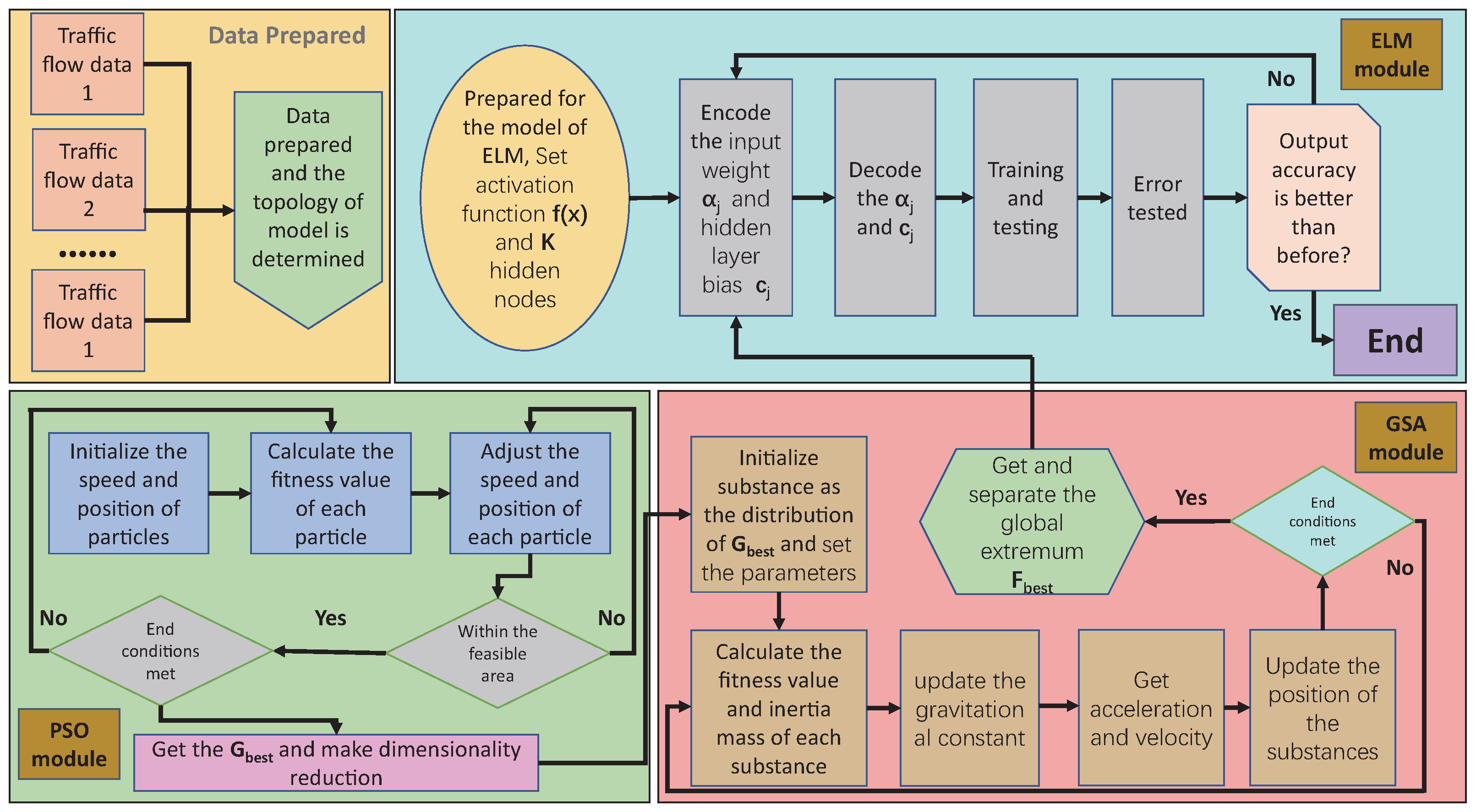
• We establish a particle swarm optimization combining a gravitational search algorithm optimized extreme learning machine model for forecasting traffic flow in the short term.
• We demonstrate the practicability of our motivation of the data-driven meta model by sufficient experiments, whose results demonstrate the outperformance of the proposed model to state-of-the-art models.

The remaining sections of this article are organized as follows. Section 2 reviews the idea of a data-driven meta-model and demonstrates a hybrid extreme learning machine optimized by combining particle swarm optimization and gravitational search algorithm. Section 3 introduces the details of our empirical study on four base datasets gathered from the expressways of Amsterdam, Netherlands. The summary of our study is given in Section 4.

2. Methodology

In this section, an extreme learning machine is applied to establish the traffic flow forecasting model first. Then, particle swarm optimization is employed for determining the parameters of the gravitational search algorithm. Later, the resulting PSOGSA hybrid module is used to optimize the extreme learning machine.

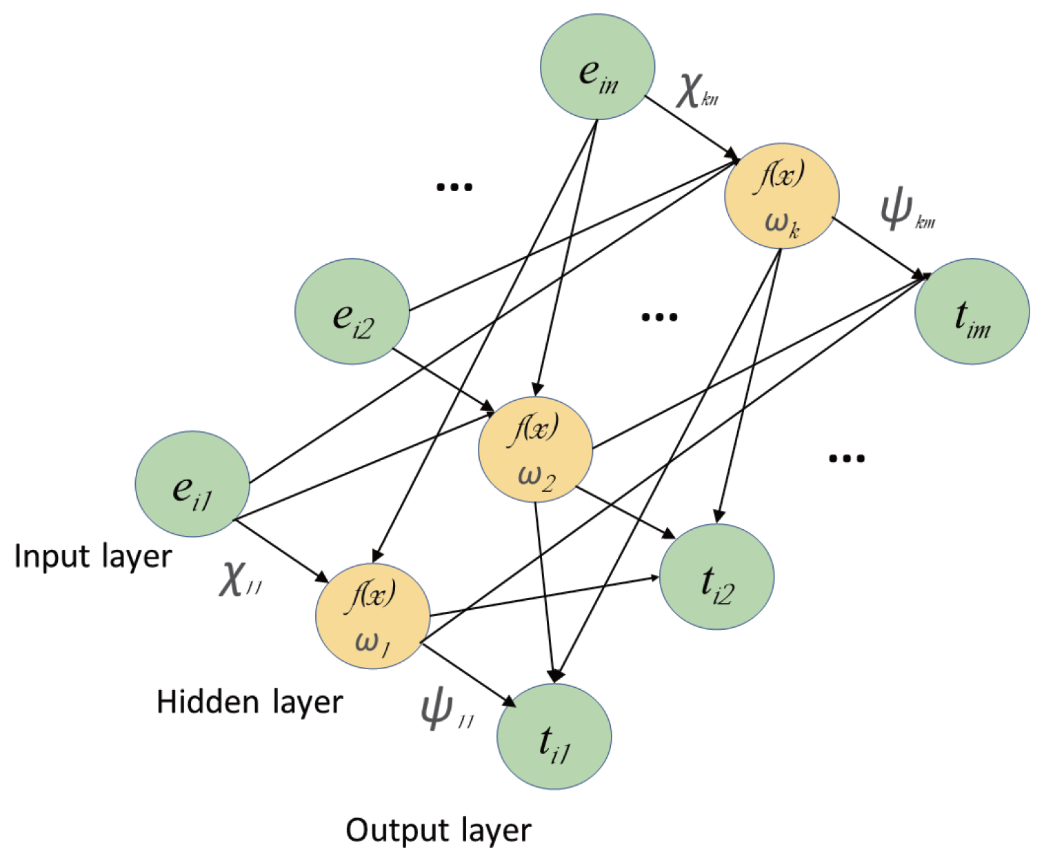
2.1. Extreme Learning Machine

Gradient descent algorithm is applied to renew the parameters in the training process of traditional neural networks. This way, the output result of the neural network can gradually approach the expected one with a decrease in the sum of square errors. There are differences between the conventional feedforward neural network and the extreme learning machine, which is a machine learning algorithm based on a feedforward neural network with a single layer. In ELM, calculating the hidden layer parameters is the approach to determining the output weight, and the hidden layer is built stochastically. This network structure makes the algorithm have faster convergence speed and lower computational complexity, and it also has advantages in fitting ability and generalization performance compared with the traditional gradient-based learning algorithm [37,38]. The standard ELM three-layer structure is shown in Figure 1.

The detailed description of ELM traffic flow forecasting model is as follows. First, the traffic flow at the ath measurement location at the ith time interval could be assumed as ${\mu }_i^{\left(a\right)}$. Then, we employ ${\left\{(e^{\left(i\right)},t^{\left(i\right)})\right\}}_{i=1}^N$ for representing N traffic flow training samples. After that, the traffic flow at the past and current $\nu -1$ time interval is set as $e^{\left(i\right)}={[{\mu }_{i-\nu +1}^{\left(a\right)},\cdots ,{\mu }_i^{\left(a\right)}]}_{a=1}^A$, in which A is the number of measurement locations and $\nu$ is the time lag. Later, the factual data of the i specimens for the traffic flow prediction model are represented by $f^{\left(i\right)}={\left[{\mu }_{i+1}^{\left(a\right)}\right]}_{a=1}^A$. The feedforward neural network with a $w_0$ hidden nodes hidden layer is demonstrated as:

$$H\beta =T,$$

(1)

in which $H={\left(g_{ij}\right)}_{i=1,\cdots ,N,j=1,\cdots ,w_0}$ indicates the output matrix of the hidden layer. Among them, $g_{ij}=f({\chi }_j^T{e}_i+{\omega }_j)$ denotes the output of the jth hidden node with regard to $e_i$. The input nodes and the jth hidden neuron could be linked by a weight vector ${\chi }_j={[{\chi }_{j1},{\chi }_{j2},\cdots ,{\chi }_{jn}]}^T$. ${\omega }_j$ represents the bias of the jth hidden neuron. The matrix of output weights is expressed as $\beta ={[{\beta }_1,{\beta }_2,\cdots ,{\beta }_{w_0}]}^T$, and we can connect the output nodes and the corresponding jth hidden neuron by the weight vector $j=1,\cdots ,w_0$. To the right of the formula, the objective matrix is denoted as $T={\left[t_1,t_2,\cdots ,t_N\right]}^T$. The operating principle of ELM is to initialize the hidden deviation and input weight randomly. Then, a rational activation function is chosen to ascertain the matrix H. After that, by calculating the least-squares (LS) solution of the linear system, which plays a role in training the feedforward neural network, the output weight $\psi$ could be calculated. The solution procedure is demonstrated as Equation (2).

$$\widehat{\beta }=H^{†}T,$$

(2)

in which $H^{†}$ denotes the Moore–Penrose (MP) generalized inverse of matrix H.

2.2. Standard Gravitational Search Algorithm

Rashedi et al. [39] proposed a novel heuristic optimization algorithm based on Newtonian laws of gravity and law of motion. In gravitational search algorithm, mutual attraction occurs between all substances under the action of gravity force. Heavier substances that may be close to the global optimal value will make other substances move toward themselves because the heavier substances have greater attraction. Consequently, the solving process of the problem to be optimized is transformed into the process of finding heavier substances [40]. Assume that v substances are distributed in a d-dimensional exploitation space; then, Equation (3) represents the position of the xth substances.

$${\alpha }_x=({\iota }_x^1,{\iota }_x^2,\cdots ,{\iota }_x^d,\cdots ,{\iota }_x^v)forx=1,2,\cdots ,v,$$

(3)

where ${\alpha }_x^d$ is the location of the xth substances in the d-dimensional space. The xth substance is gravitated by the yth substance at the $t_0$th iteration, as shown in Equation (4).

$$F_{xy}^d\left(t_0\right)=G\left(t_0\right)\frac{M_y\left(t_0\right)\times M_x\left(t_0\right)}{Z_{xy}\left(t_0\right)+\delta }({\iota }_y^d\left(t_0\right)-{\iota }_x^d\left(t_0\right)),$$

(4)

in which $M_x\left(t_0\right)$ is the inertial masses of the substance x which is affected by gravity, and the force producing substance y is represented as $M_y\left(t_0\right)$. $\delta$ denotes a tiny appropriate constant and the Euclidian distance between substance x and substance y is $Z_{xy}\left(t_0\right)$. $G\left(t\right)=G_0{e}^{-\zeta \left(\frac{t_0}{S}\right)}$ represents a gravity constant which gradually decreases during the iteration process, and it is also the controller of the optimized accuracy process. S represents the total iterations, $\zeta$ denotes the manually adjusted constant, and the initial value of $G_s$ is $G_0$. The total gravity acting on the xth substance is the stochastic weighted sum of the force applied from another substance in the dth dimension.

$$F_{xy}^d\left(t_0\right)=\sum _{y=1,y\ne x}^{v}ran{d}_y{F}_{xy}^d\left(t_0\right),$$

(5)

where $ran{d}_y\in (0,1)$ denotes a stochastic value employed for increasing the stochastic features of GSA. A global search tactic on the solution space is applied to keep the GSA from sinking into the local minima at the beginning of the optimization process. Then, the global exploitation fades out and local exploitation fades in with the running of the algorithm.

In the process of standardizing exploration and exploitation, the optimization ability of GSA could be improved. After that, the number of the agent is decreased to maintain the balance of exploitation and exploration. Other substances are subjected to gravity from a group of substances with larger mass (${\lambda }_{best}$ corresponding optimal solution) [39]. Equation (6) could strengthen the performance of GSA, whereas by the time function, ${\lambda }_{best}$ decreases with the increase of the number of iterations.

$$F_{xy}^d\left(t_0\right)=\sum _{y\ne x,y\in {\lambda }_{best}}^{v}ran{d}_y{F}_{xy}^d\left(t_0\right).$$

(6)

The acceleration of substance x at time $t_0$ in the d-dimension is shown as Equation (7) based on Newton’s second theorem.

$$a_x^d\left(t_0\right)=\frac{F_x^d\left(t_0\right)}{M_x\left(t_0\right)},$$

(7)

where $M_x\left(t_0\right)$ is the inertial mass of the xth substance. The velocity and direction of the substance are regulated by the acceleration function. The velocity and position of the substance is updated under the guidance of Equations (8) and (9) in every iteration.

$$v_x^d(t_0+1)=ran{d}_x\times v_x^d\left(t_0\right)+a_x^d\left(t_0\right),$$

(8)

$${\iota }_x^d(t_0+1)={\iota }_x^d\left(t_0\right)+v_x^d(t_0+1).$$

(9)

In Equation (9), the position and speed of the substance at the $t_0$th iteration is denoted as $v_x^d\left(t_0\right)$ and ${\iota }_x^d\left(t_0\right)$. Then, we can calculate the inertia mass according to the size of the fitness value. The distance between the substance and the optimal value decreases with the increase of its inertial mass, which demonstrates that the attraction of the substance is inversely proportional to its moving velocity. Later, the inertial mass of the substance is updated as following:

$$m_x\left(t_0\right)=\frac{fi{t}_x\left(t_0\right)-worst\left(t_0\right)}{best\left(t_0\right)-worst\left(t_0\right)},$$

(10)

$$M_x\left(t_0\right)=\frac{m_x\left(t_0\right)}{{\sum }_{y=1}^v{m}_x\left(t_0\right)},$$

(11)

in which

$$worst\left(t_0\right)=\underset{x\in 1,2,\cdots v}{max}fi{t}_x\left(t_0\right),$$

(12)

$$best\left(t_0\right)=\underset{x\in 1,2,\cdots v}{min}fi{t}_x\left(t_0\right),$$

(13)

and where $fi{t}_x\left(t_0\right)$ denotes the fitness value of the xth substances at time $t_0$.

2.3. Standard Particle Swarm Optimization

According to the observation of the social behavior of biological organisms, Kennedy and Eberhart propose an evolutionary computation algorithm termed particle swarm optimization (PSO) [41]. PSO explores the best solution in the specified search space through free-flying particles. These particles could be regarded as candidate solutions, and seeking the best particle in the path is the process of seeking the best solution. That is to say, the best solution found so far has the same performance as the independent solution of each particle.

In D-dimensional space, a population composed of $N_0$ particles can be assumed as $P=(P_1,P_2,\cdots ,P_{n0})$, in which the lth particle is denoted as a D-dimensional vector $P_l={[p_{l1},p_{l2},\cdots ,p_{lD}]}^T$. The advantages and disadvantages of the current position can be determined according to the calculation results of the fitness value corresponding to the particle position $P_l$, based on the objective function. There is a speed representing the direction and the distance of each particle. $\rho ={[{\rho }_{l1},{\rho }_{l2},\cdots ,{\rho }_{lD}]}^{{}_T}$ denotes the speed of the th particle. The position and speed of the particles are updated in each iteration of the PSO, as shown in the following:

$${\rho }_{ld}^{g+1}=\varphi {\rho }_{ld}^g+w_1{\kappa }_1(q_d^v-p_{ld}^v),$$

(14)

$$p_{ld}^{g+1}=p_{ld}^g+{\rho }_{ld}^{g+1},$$

(15)

in which $Q={[q_1,q_2,\cdots ,q_D]}^T$ is the global best position of colony and $Q_l={[q_{l1},q_{l2},\cdots ,q_{lD}]}^T$ is the individual best position of the ith particle. The inertia weight is $\varphi$ and the number of hidden layer nodes is g. $w_1$ and $w_2$ are employed for representing the factors of learning. The range of the speed is denoted as $[v_{0min},v_{0max}]$ and terms ${\kappa }_1$ and ${\kappa }_2$ are stochastically ascertained in range U(0,1).

2.4. ELM Optimization Learning Based on Data Driven

The installation of the ELM network structure has a non-negligible influence on the forecasting accuracy of the traffic flow model. In this article, we employ PSO instead of the original random method for generating the initial population of GSA, to improve its performance. Then, the hybrid evolutionary algorithm is employed for completing the data-driven optimization tasks, which are transformed from a selection of input weight and hidden layer threshold in ELM. Figure 2 demonstrates the workflow of the obtained data-driven traffic flow forecasting model, which is termed the PSOGSA-ELM model.

3. Experiments

3.1. Data Description

In this section, four benchmark traffic datasets are employed for appraising the PSOGSA-ELM model. Wang et al. [42] collect these datasets from four freeways A1, A2, A4, and A8, which end at Amsterdam A10 Ring Road. MONICA loop detectors are employed for collecting these datasets from 20 May to 24 June 2010, and the detection location is demonstrated in Figure 3.

The raw traffic flow data are summarized by rolling stocks every hour per minute, which consists of five weeks. The following is the fundamental message of the four motorways.

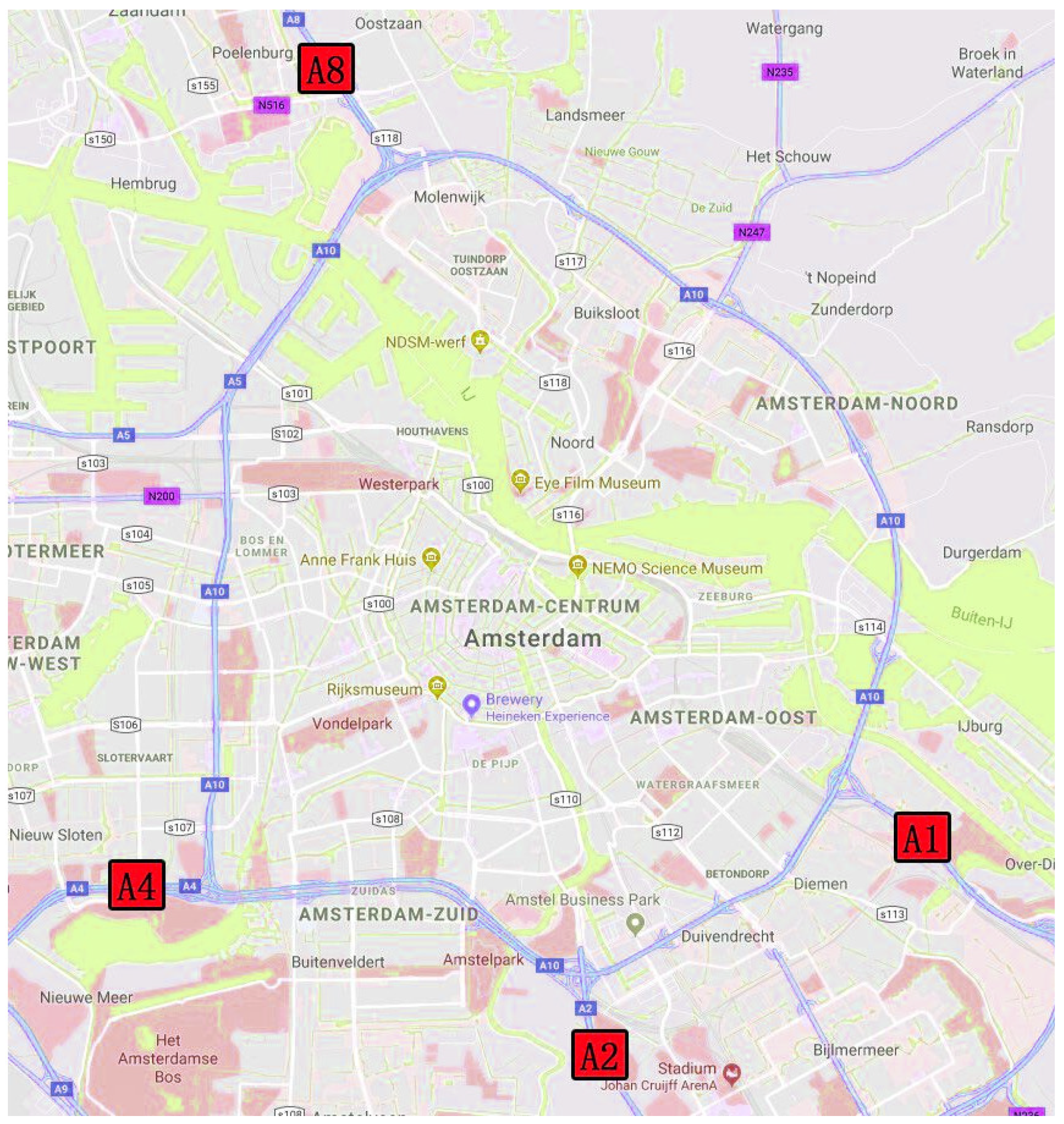
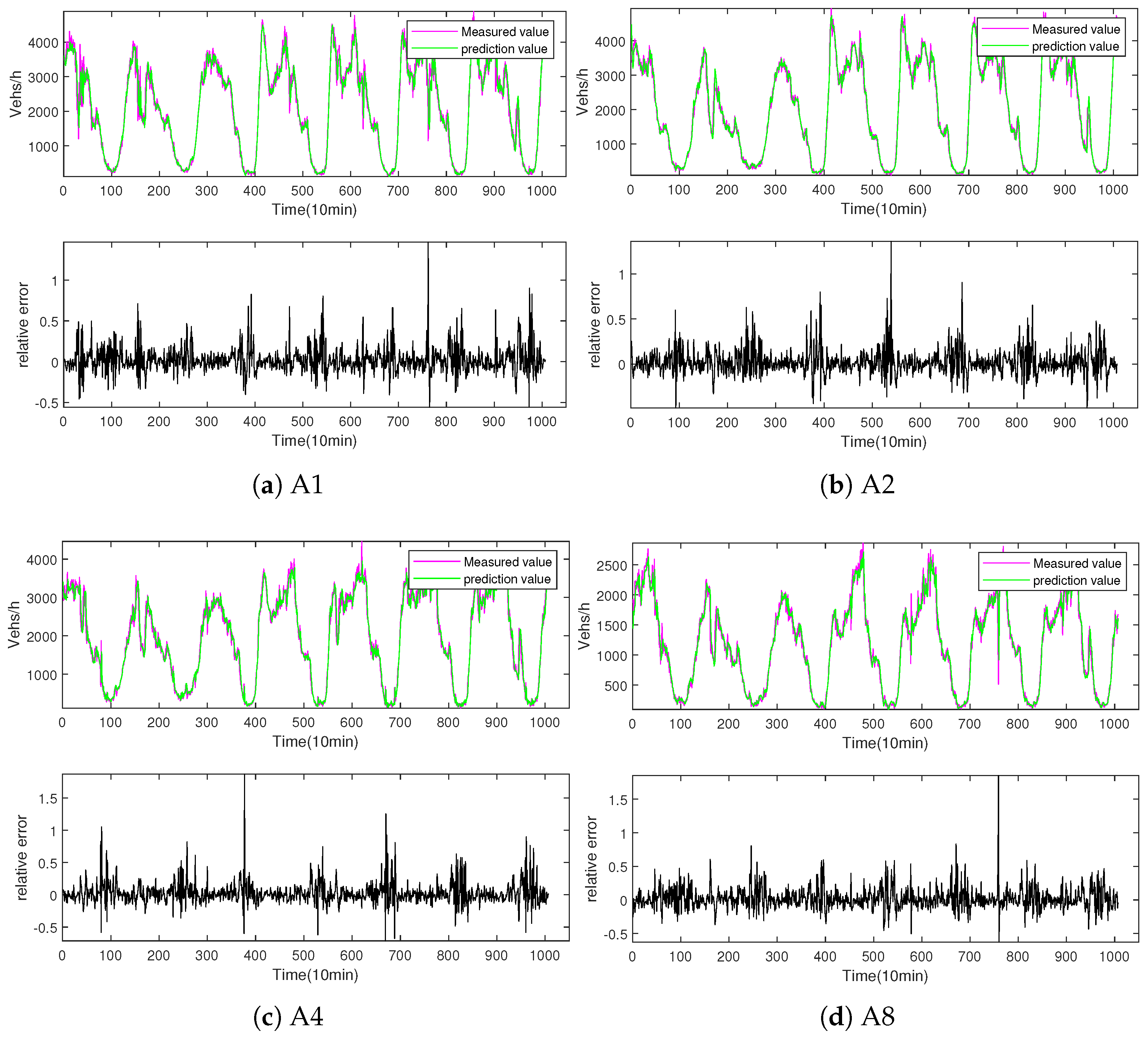
• The A1 freeway is an extremely significant route in Europe whose extraordinary position is the link between the German border and Amsterdam. The first 3+ barrier-separated lanes with high-occupancy vehicle (HOV) in Europe is located on the A1 freeway. Therefore, forecasting traffic flow accurately is thrown down the gauntlet because the flow on an HOV vehicle lane changes dramatically over time.
• The A2 expressway links the Belgian border and the city of Amsterdam, which is one of the expressways with the highest traffic flow in the Netherlands. The data collected before the road widening in 2010 could be employed for evaluating the performance of the proposed framework when the road falls into traffic congestion in our research.
• As a section of the Rijksweg 4, the A4 expressway in the Netherlands is another high priority, starting from Amsterdam and ending at the Belgian border.
• A8 is the shortest of the four freeways, starting from the A10 motorway at interchange Coenplein to the Zaandijk, and the total length is less than 10 km.

Li et al. [43] proposed a statistical learning method, which is applied for correcting and complementing the missing values in the original data collected by the detector.

3.2. Evaluation Criterion

In this article, two frequently used criteria are applied to test the forecasting performance. The root means square error (RMSE) demonstrates the average difference between the predictive value and the measured value. The mean absolute percentage error (MAPE) calculates the percentage of the differences. The mathematical definitions of the two criteria are shown in Equations (16) and (17), respectively.

$$\mathrm{RMSE}=\sqrt{\frac{1}{P_0}\sum _{p_0=1}^{P_0}{\left(\widehat{u}\left(p_0\right)-u\left(p_0\right)\right)}^2},$$

(16)

$$\mathrm{MAPE}=\frac{1}{P_0}\sum _{p_0=1}^{P_0}\left|\frac{\widehat{u}\left(p_0\right)-u\left(p_0\right)}{u\left(p_0\right)}\right|\times 100\%,$$

(17)

where $\widehat{u}\left(p_0\right)$ and $u\left(p_0\right)$ denote the predictive value and the measured value of the $p_0$th sample.

3.3. Performance Evaluation

To assess the prediction performance of PSOGSA-ELM, we compare the proposed model with some traffic flow models which are commonly applied in the intelligent transportation system.

Historical average (HA): HA is employed for forecasting the average of the identical time on an identical day in the weeks before a given time in a day.

Exponential smoothing (ES): Exponential smoothing (ES) is a particular weighted moving average method (MA), which is an important category of time series analysis and prediction methods [44]. The forecasted values during the observation period are further affected by the recently observed values due to the unequal weights given by the observed values at various times. To mirror the flatness of the trend change, we employ the double exponential smoothing method for setting parameter ${\alpha }_0$ in the model to 0.4.

Artificial neural network (ANN): ANN is a kind of nonparametric learning model with a single hidden layer neural network structure. According to the network parameters criteria in [45], we set the MSE target value as 0.001, the maximum number of neurons as 40, the number of hidden layers as 1, and the expansion speed of the radial basis function as 2000. Based on the default value, 25 neurons are set to add between displays.

Decision trees (DTs): The DT model, which is based on the classification and regression tree (CART), is employed for forecasting traffic flows in our experiment. In CART, the robustness against missing data and noise is strong, and the prior hypothesis is not necessary. The detailed knowledge about CART is in [46].

Autoregression (AR): The AR has been widely applied to forecasting traffic flow as a linear regression model. In AR, the linear combination of stochastic variables at a previous moment is employed for describing the random variables at a later moment, and then, the randomness of traffic flow could be handled effectively. We set the parameter $\widehat{p}$ from 0 to 8 according to the suggestion in [20].

Seasonal autoregressive integrated moving average (SARIMA): In the data collected regularly, there are usually sequential lag relationships, whose correlation could be further excavated and applied by the SARIMA model for forecasting the traffic flow [35]. We set the parameters of the model as SARIMA $(1,0,1)\times {(0,1,1)}_{1008}$, ${\varphi }_0=0.8$, ${\theta }_0=0.4$, ${\mathsf{\Theta }}_0=0.8$.

Support vector machine regression (SVR): The detailed description of SVR is in [20]. In our experiment, the kernel function of the SVR model is selected as the radial basis function (RBF). The maximum difference between traffic flow determines the cost parameter $\widehat{C}$, in which the regression horizon is set to 8.

To prove the optimized capability of the hybrid data-driven model, the ELM optimized by genetic algorithm (GA-ELM) and the standard extreme learning machine is compared with the proposed model. Since substances are randomly distributed in GA and hybrid PSOGSA, each run will generate different results. Therefore, the outcomes of 100 runs are regarded as the outcomes on every benchmark dataset for the GA-ELM model and the PSOGSA-ELM model in this comparative experiment.

We can find in

Table 1. The RMSE (vehs/h) of different forecasting models on datasets collected from A1, A2, A4, and A8, respectively.

Model	A1	A2	A4	A8
HA	404.84	348.96	357.85	218.72
ES	315.82	226.40	237.76	174.67
ANN	299.64	212.95	225.86	166.50
DT	316.57	224.79	243.19	238.35
AR	301.44	214.22	226.12	166.71
SARIMA	308.44	221.08	228.36	169.36
SVR	329.09	259.74	253.66	190.30
ELM	300.67	208.84	224.54	172.69
GA-ELM	291.42	211.43	228.57	169.25
PSOGSA-ELM	288.03	204.09	220.52	163.92

and

Table 2. The MAPE (%) of different forecasting models on datasets collected from A1, A2, A4, and A8, respectively.

Model	A1	A2	A4	A8
HA	16.87	15.53	16.72	16.24
ES	11.94	10.75	11.97	12.00
ANN	12.61	10.89	12.49	12.53
DT	12.08	10.86	12.34	13.62
AR	13.57	11.59	12.70	12.71
SARIMA	12.81	11.25	12.05	12.44
SVR	14.34	12.22	12.23	12.48
ELM	11.92	10.32	12.09	12.58
GA-ELM	11.86	10.30	11.87	12.26
PSOGSA-ELM	11.53	10.16	11.67	12.02

that the PSOGSA-ELM has remarkable advantages in forecasting the performance of all four benchmark datasets.

As shown in Table 1, the RMSEs of proposed model are $12.48\%$, $21.42\%$, $13.06\%$, and $13.86\%$ lower than the RMSEs of SVR at A1, A2, A4, and A8, respectively. The RMSEs of the proposed model are $8.80\%$, $9.85\%$, $7.25\%$, and $6.15\%$ lower than the RMSEs of ES at A1, A2, A4, and A8, respectively. The RMSEs of the proposed model are $3.87\%$, $4.16\%$, $2.36\%$, and $1.55\%$ lower than the RMSEs of ANN, at A1, A2, A4, and A8, respectively. As shown in Table 2, the MAPEs of the proposed model are $8.82\%$, $8.89\%$, $3.15\%$, and $3.38\%$ lower than the MAPEs of SARIMA at A1, A2, A4, and A8, respectively. The MAPEs of the proposed model are $3.27\%$, $1.55\%$, $3.47\%$, and $4.45\%$ lower than the MAPEs of standard ELM at A1, A2, A4, and A8, respectively. The MAPEs of the proposed model are $2.78\%$, $1.36\%$, $1.68\%$, and $1.96\%$ lower than the MAPEs of GA-ELM at A1, A2, A4, and A8, respectively.

Then, Akaike Information Criterion (AIC) is introduced into our experiment, as demonstrated in

Table 3. Comparative experiment on AICc.

Model	A1	A2	A4	A8
ELM	15.429	15.544	15.168	14.267
GA-ELM	15.416	15.522	15.136	14.161
PSOGSA-ELM	15.325	15.430	15.055	14.156

.

AIC includes both simplicity and accuracy as references while evaluating the performance of different models [47,48]. In Table 3, we discover that the AIC of the PSOGSA-ELM model is the smallest of the three models related to ELM. That is to say, our proposed model performs better in terms of accuracy and simplicity.

In Figure 4a–d, the deviation between the short-term traffic flow predicted values of the model and the practical measured values are visualized intuitively. The purple lines demonstrate the measured values, whereas the green lines represent the predicted values. The errors between the predicted value and measured value divided by the ground truth, termed the relative error of the model, are plotted with a black line. In Figure 4, we can find the related errors calculated by experiments approached 0 most of the time, which proved the outstanding performance of the PSOGSA-ELM model in the scenes of A1, A2, A4, and A8.

In addition, an evaluation index dedicated to traffic flow forecasting, termed GEH statistics [49,50,51], is also employed for analyzing the results.

Table 4. GEH statistics of the GSA-ELM model.

Dataset	A1	A2	A4	A8
GEH	6.13	4.48	4.88	4.81

lists the GEH statistics value of the prediction outcomes of proposed models on four base datasets.

In Table 4, we can find that the GEH of the prediction results for most benchmark datasets is less than 5. On the A1 dataset, the value of GEH is 6.12, which is probably because the A1 dataset has stronger volatility than the other three datasets. The fitting performance of the model is in good accordance with the evaluation standard of GEH.

3.4. Ablation Study

The fluctuation of traffic flow over a continuous time rather than minute-to-minute fluctuation is the object of traffic flow forecasting study [21,42]. Consequently, we regard the traffic flow data aggregation of a 1-min average in the subsequent 10 min as the 10-min data and employ it for forecasting tasks. The original data made of 5 weeks of measurement is classified as a training set and testing set in our experiment. The training set includes the samples in the first four weeks and the testing set consists of the samples in the fifth week, whereas the number of samples measured every week is 1008. The time interval is stipulated as 8 and hidden layer nodes of ELM are set to 30. On this basis, we apply the classical sigmoid function as the activation function. The specific parameter settings of PSO and GSA are shown in

Table 5. The parameters setting of GSA module and PSO.

Algorithm	Paramater	Value
PSO	Range of inertia weights	[0.4,0.9]
	Number of particles	40
	$c1$	1.7
	$c2$	1.3
	Maximum Iterations	150
GSA	Population size	300
	$G_0$	100
	$\upsilon$	20
	Maximum Iterations	100

. MAPE and RMSE are employed for evaluating the optimization performance of PSOGSA. The trend for the forecasting performance corresponding to the number of algorithm iterations is demonstrated in Figure 5. In Table 5, it obvious that the values of RMSE and MAPE both tend to smooth when the number of iterations is more than 80, which testifies to the rationality of setting the maximum number of iterations of the GSA module as 100.

For evaluating the ability of PSOGSA to optimize ELM network structure parameters based on data-driven methods, we introduce a genetic algorithm (GA), which is a popular optimization algorithm, to our comparative experiment. The non-specific parameters of GA are set to be the same as PSOGSA for a fair comparison. The number of iterations of GA is also stipulated as 100, whereas the variation probability is $0.03$, the generation gap is $0.95$ and the crossover probability is $0.85$. Detailed information on the genetic algorithm optimized ELM (GA-ELM) is shown in [52]. As two characteristic periods, the morning peak and afternoon peak are chosen for evaluating the optimization performance of PSOGSA and GA in determining the parameter of ELM. Among them, the time interval from 7:30 to 9:30 represents the morning peak and that from 13:30 to 14:30 represents the afternoon peak.

Table 6. The forecasting performance during the morning peak period while optimizing ELM with different optimization algorithms.

The Morning Peak Period	Groundtruth	ELM	Prediction GA-ELM	PSOGSA-ELM
6/11/7:30	3546	3274.033	3270.369	3392.933
6/11/8:30	3792	3700.290	3724.208	3756.983
6/11/9:30	4184	3691.265	3734.778	3801.143
6/14/7:30	2670	2641.334	2662.170	2649.311
6/14/8:30	3116	2934.568	2957.073	2976.761
6/14/9:30	3094	3005.691	3023.728	3033.094
6/15/7:30	2817	2999.734	3012.434	2920.417
6/15/8:30	2893	2846.403	2808.657	2807.973
6/15/9:30	3154	3225.806	3200.339	3239.240
RMSE		217.03	206.39	164.44
MAPE		5.01	4.69	3.76

and

Table 7. The forecasting performance during the afternoon peak period while optimizing ELM with different optimization algorithms.

The Afternoon Peak Period	Groundtruth	ELM	Prediction GA-ELM	PSOGSA-ELM
6/11/13:30	3948	3957.867	3973.349	3956.204
6/11/14:00	4373	4179.630	4437.895	44,407.233
6/11/14:30	3542	3976.427	4030.626	3968.726
6/14/13:30	3817	3369.284	3346.841	3376.680
6/14/14:00	4135	3734.672	3744.345	3812.346
6/14/14:30	4197	4261.105	4384.840	4272.334
6/15/13:30	3732	3394.333	3430.046	3431.599
6/15/14:00	4032	3818.189	3842.358	3827.597
6/15/14:30	4549	3895.383	3947.706	3908.953
RMSE		361.78	356.10	338.08
MAPE		7.62	7.57	6.82

demonstrate the forecasting performances of three types of models during the morning and afternoon high peak periods, respectively.

In Figure 6 and Figure 7, the forecasting error, which is the absolute value of the measurement minus the forecasting, is shown in two categories: the morning and the afternoon rush hour, respectively. Table 6 and Table 7 demonstrate that the RMSE and MAPE of the PSOGSA-ELM model are lower than the other comparable models in these periods. In Figure 6 and Figure 7, the PSOGSA-ELM model realizes a lower forecasting error than other comparison models in different scenarios. Thus, the network structure of the ELM model could be optimized by hybrid PSOGSA better than GA during the high peak period in the morning and afternoon. Moreover, we also consider the traffic flow in a low traffic period. Midnight in the morning, covering the period from 23:30 to 00:30 is considered the low traffic period in our experiment. During this time, the violent fluctuation of RMSE could be caused by a small forecasting error.

When the traffic flow is low at midnight, the prediction results from ELM optimized by different algorithms are shown in

Table 8. The forecasting performance during the low traffic period at midnight while optimizing ELM with different optimization algorithms.

The Midnight Period	Ground Truth	ELM	Prediction GA-ELM	PSOGSA-ELM
6/11/23:30	297	235.481	238.125	238.980
6/12/00:00	243	236.766	233.857	241.629
6/12/00:30	229	337.797	313.061	309.774
6/12/23:30	297	264.544	247.249	259.573
6/13/00:00	192	232.681	243.316	212.192
6/13/00:30	426	402.075	342.899	374.851
6/13/23:30	241	246.560	236.844	236.777
6/14/00:00	187	336.153	323.598	261.377
6/14/00:30	284	368.125	335.396	316.246
RMSE		73.25	69.88	48.20
MAPE		24.47	24.02	15.93

. Figure 8 shows the forecasting errors of three models during this period, which illustrates that PSOGSA is better than the genetic algorithm in determining the network parameters of ELM. Consequently, the optimization performance for the ELM of hybrid PSOGSA is better than GA under different traffic flow situations. To further reduce the stochasticity of the prediction performances, the traffic flow in more diversified periods is employed for a comparative experiment of several models, as shown in Figure 9.

To assess the comprehensive performance of the hybrid model proposed in this article, ELM, GA-ELM, and PSOGSA-ELM are selected for a comparative experiment about running time. In

Table 9. The computational time of ELM, GA-ELM, and GSA-ELM.

Model	Computational Time (s)
ELM	0.0516
GA-ELM	100.2139
PSOGSA-ELM	83.8456

, we can find that the running time of ELM is the fastest of the three due to its random parameter generation process. Nevertheless, the target of the data-driven model, minimizing the forecasting error, could hardly be realized by randomly generated parameters. Meanwhile, on the basis of determining the parameters reasonably of the forecasting model, PSOGSA-ELM still maintains a low running time, which is lower than GA-ELM. The training of the proposed model costs about 83 seconds in our experiments on the benchmark dataset. Fortunately, we only need to train the model one time. The forecasting time of the proposed model is the same as the general extreme learning machine, i.e., less than 0.1 second. The parameters of the proposed model are automatically optimized in a data-driven fashion, and the only required input is traffic flow data. Therefore, the algorithm can be effectively applied to other traffic scenes at different locations without human interaction.

With accurate predicted future traffic flow, the policymakers can adjust the time slice of the traffic lights to make perspective traffic management based on the future traffic flow for effective leverage of the road resources. The policymakers can also adjust the driving rules to control the traffic on the road network to optimize the allocation and management of road resources. Moreover, the spreading of the future traffic flow by public media can also induce vehicles to choose alternative ways spontaneously to improve the traffic conditions.

4. Conclusions

In this paper, we develop a two-stage data-driven hybrid extreme learning model for short-term traffic flow forecasting. Comparative experiments on the trained model show that the RMSEs of the proposed model are $3.87\%$, $4.16\%$, $2.36\%$, and $1.55\%$ lower than the RMSEs of the state-of-the-art model, at four benchmark datasets, respectively. The MAPEs of the proposed model are $2.78\%$, $1.36\%$, $1.68\%$, and $1.96\%$ lower than the MAPEs of the state-of-the-art model at four benchmark datasets, respectively. Consequently, the experimental results demonstrate the model can automatically determine the optimal hyperparameters of the extreme learning machine in a data-driven fashion. Since the hyperparameters of the model are optimized automatically in a data-driven manner, the model can be conveniently deployed to different intelligent traffic systems without human intervention. In the future, we will improve forecasting accuracy by spatiotemporal learning on other models.

References

1. Cai, L.; Lei, M.; Zhang, S.; Yu, Y.; Zhou, T.; Qin, J. A noise-immune lstm network for short-term traffic flow forecasting. Chaos Interdiscip. J. Nonlinear Sci. 2020, 30, 023135. [Google Scholar] [CrossRef] [PubMed]
2. Olayode, I.O.; Tartibu, L.K.; Okwu, M.O.; Ukaegbu, U.F. Development of a hybrid artificial neural network-particle swarm optimization model for the modelling of traffic flow of vehicles at signalized road intersections. Appl. Sci. 2021, 11, 8387. [Google Scholar] [CrossRef]
3. Li, Z.; Cao, Q.; Zhao, Y.; Zhuo, R. Signal cooperative control with traffic supply and demand on a single intersection. IEEE Access 2018, 6, 54407–54416. [Google Scholar]
4. Li, Z.; Cao, Q.; Zhao, Y.; Tao, P.; Zhuo, R. Krill herd algorithm for signal optimization of cooperative control with traffic supply and demand. IEEE Access 2019, 7, 10776–10786. [Google Scholar]
5. Chen, L.; Yang, D.; Zhang, D.; Wang, C.; Li, J. Deep mobile traffic forecast and complementary base station clustering for C-RAN optimization. J. Netw. Comput. Appl. 2018, 121, 59–69. [Google Scholar] [CrossRef] [Green Version]
6. Ahmed, M.S.; Cook, A.R. Analysis of Freeway Traffic Time-Series Data by Using Box-Jenkins Techniques. Number 722. 1979. Available online: https://trid.trb.org/view/148123 (accessed on 9 May 2022).
7. Yang, H.; Li, X.; Qiang, W.; Zhao, Y.; Zhang, W.; Tang, C. A network traffic forecasting method based on SA optimized ARIMA–BP neural network. Comput. Netw. 2021, 193, 108102. [Google Scholar] [CrossRef]
8. Cai, L.; Zhang, Z.; Yang, J.; Yu, Y.; Zhou, T.; Qin, J. A noise-immune Kalman filter for short-term traffic flow forecasting. Phys. A Stat. Mech. Appl. 2019, 536, 122601. [Google Scholar] [CrossRef]
9. Zhou, T.; Jiang, D.; Lin, Z.; Han, G.; Xu, X.; Qin, J. Hybrid dual Kalman filtering model for short-term traffic flow forecasting. IET Intell. Transp. Syst. 2019, 13, 1023–1032. [Google Scholar] [CrossRef]
10. Olayode, I.O.; Tartibu, L.K.; Okwu, M.O. Prediction and modeling of traffic flow of human-driven vehicles at a signalized road intersection using artificial neural network model: A South African road transportation system scenario. Transp. Eng. 2021, 6, 100095. [Google Scholar] [CrossRef]
11. Olayode, I.O.; Severino, A.; Campisi, T.; Tartibu, L.K. Prediction of Vehicular Traffic Flow using Levenberg-Marquardt Artificial Neural Network Model: Italy Road Transportation System. Commun.-Sci. Lett. Univ. Zilina 2022, 24, E74–E86. [Google Scholar] [CrossRef]
12. Cai, L.; Yu, Y.; Zhang, S.; Song, Y.; Xiong, Z.; Zhou, T. A sample-rebalanced outlier-rejected k-nearest neighbor regression model for short-term traffic flow forecasting. IEEE Access 2020, 8, 22686–22696. [Google Scholar] [CrossRef]
13. Cai, L.; Chen, Q.; Cai, W.; Xu, X.; Zhou, T.; Qin, J. SVRGSA: A hybrid learning based model for short-term traffic flow forecasting. IET Intell. Transp. Syst. 2019, 13, 1348–1355. [Google Scholar] [CrossRef]
14. Zheng, S.; Zhang, S.; Song, Y.; Lin, Z.; Jiang, D.; Zhou, T. A noise-immune boosting framework for short-term traffic flow forecasting. Complexity 2021, 2021, 5582974. [Google Scholar] [CrossRef]
15. Cai, W.; Yang, J.; Yu, Y.; Song, Y.; Zhou, T.; Qin, J. PSO-ELM: A hybrid learning model for short-term traffic flow forecasting. IEEE Access 2020, 8, 6505–6514. [Google Scholar] [CrossRef]
16. Cui, Z.; Huang, B.; Dou, H.; Tan, G.; Zheng, S.; Zhou, T. GSA-ELM: A hybrid learning model for short-term traffic flow forecasting. IET Intell. Transp. Syst. 2022, 16, 41–52. [Google Scholar] [CrossRef]
17. Hu, X.; Xu, X.; Xiao, Y.; Chen, H.; He, S.; Qin, J.; Heng, P.A. SINet: A scale-insensitive convolutional neural network for fast vehicle detection. IEEE Trans. Intell. Transp. Syst. 2018, 20, 1010–1019. [Google Scholar] [CrossRef] [Green Version]
18. Xu, X.; Yu, T.; Hu, X.; Ng, W.W.; Heng, P.A. SALMNet: A structure-aware lane marking detection network. IEEE Trans. Intell. Transp. Syst. 2020, 22, 4986–4997. [Google Scholar] [CrossRef]
19. Li, L.; Lin, Y.; Du, B.; Yang, F.; Ran, B. Real-time traffic incident detection based on a hybrid deep learning model. Transp. A Transp. Sci. 2022, 18, 78–98. [Google Scholar] [CrossRef]
20. Zhou, T.; Han, G.; Xu, X.; Lin, Z.; Han, C.; Huang, Y.; Qin, J. δ-agree AdaBoost stacked autoencoder for short-term traffic flow forecasting. Neurocomputing 2017, 247, 31–38. [Google Scholar] [CrossRef]
21. Zhou, T.; Han, G.; Xu, X.; Han, C.; Huang, Y.; Qin, J. A learning-based multimodel integrated framework for dynamic traffic flow forecasting. Neural Process. Lett. 2019, 49, 407–430. [Google Scholar] [CrossRef]
22. Li, L.; Qin, L.; Qu, X.; Zhang, J.; Wang, Y.; Ran, B. Day-ahead traffic flow forecasting based on a deep belief network optimized by the multi-objective particle swarm algorithm. Knowl.-Based Syst. 2019, 172, 1–14. [Google Scholar] [CrossRef]
23. Qu, Z.; Li, H.; Li, Z.; Zhong, T. Short-term traffic flow forecasting method with MB-LSTM hybrid network. IEEE Trans. Intell. Transp. Syst. 2020, 23, 225–235. [Google Scholar]
24. Lu, H.; Ge, Z.; Song, Y.; Jiang, D.; Zhou, T.; Qin, J. A temporal-aware lstm enhanced by loss-switch mechanism for traffic flow forecasting. Neurocomputing 2021, 427, 169–178. [Google Scholar] [CrossRef]
25. Fang, W.; Zhuo, W.; Yan, J.; Song, Y.; Jiang, D.; Zhou, T. Attention meets long short-term memory: A deep learning network for traffic flow forecasting. Phys. A Stat. Mech. Appl. 2022, 587, 126485. [Google Scholar] [CrossRef]
26. Luo, X.; Peng, J.; Liang, J. Directed hypergraph attention network for traffic forecasting. IET Intell. Transp. Syst. 2022, 16, 85–98. [Google Scholar] [CrossRef]
27. Li, L.; He, S.; Zhang, J.; Ran, B. Short-term highway traffic flow prediction based on a hybrid strategy considering temporal–spatial information. J. Adv. Transp. 2016, 50, 2029–2040. [Google Scholar] [CrossRef]
28. Lu, H.; Huang, D.; Song, Y.; Jiang, D.; Zhou, T.; Qin, J. St-trafficnet: A spatial-temporal deep learning network for traffic forecasting. Electronics 2020, 9, 1474. [Google Scholar] [CrossRef]
29. Li, S.; Zhuang, C.; Tan, Z.; Gao, F.; Lai, Z.; Wu, Z. Inferring the trip purposes and uncovering spatio-temporal activity patterns from dockless shared bike dataset in Shenzhen, China. J. Transp. Geogr. 2021, 91, 102974. [Google Scholar] [CrossRef]
30. Yang, S.; Li, H.; Luo, Y.; Li, J.; Song, Y.; Zhou, T. Spatiotemporal Adaptive Fusion Graph Network for Short-Term Traffic Flow Forecasting. Mathematics 2022, 10, 1594. [Google Scholar] [CrossRef]
31. Dou, H.; Tan, J.; Wei, H.; Wang, F.; Yang, J.; Ma, X.G.; Wang, J.; Zhou, T. Transfer inhibitory potency prediction to binary classification: A model only needs a small training set. Comput. Methods Programs Biomed. 2022, 215, 106633. [Google Scholar] [CrossRef]
32. Zhou, T.; Dou, H.; Tan, J.; Song, Y.; Wang, F.; Wang, J. Small dataset solves big problem: An outlier-insensitive binary classifier for inhibitory potency prediction. Knowl.-Based Syst. 2022. [Google Scholar] [CrossRef]
33. Ahila, R.; Sadasivam, V.; Manimala, K. An integrated PSO for parameter determination and feature selection of ELM and its application in classification of power system disturbances. Appl. Soft Comput. 2015, 32, 23–37. [Google Scholar] [CrossRef]
34. Huang, G.B.; Zhu, Q.Y.; Siew, C.K. Extreme learning machine: Theory and applications. Neurocomputing 2006, 70, 489–501. [Google Scholar] [CrossRef]
35. Lippi, M.; Bertini, M.; Frasconi, P. Short-term traffic flow forecasting: An experimental comparison of time-series analysis and supervised learning. IEEE Trans. Intell. Transp. Syst. 2013, 14, 871–882. [Google Scholar] [CrossRef]
36. Hu, W.; Yan, L.; Liu, K.; Wang, H. A short-term traffic flow forecasting method based on the hybrid PSO-SVR. Neural Process. Lett. 2016, 43, 155–172. [Google Scholar] [CrossRef]
37. Lv, L.; Wang, W.; Zhang, Z.; Liu, X. A novel intrusion detection system based on an optimal hybrid kernel extreme learning machine. Knowl.-Based Syst. 2020, 195, 105648. [Google Scholar] [CrossRef]
38. Manoharan, J.S. Study of variants of Extreme Learning Machine (ELM) brands and its performance measure on classification algorithm. J. Soft Comput. Paradig. (JSCP) 2021, 3, 83–95. [Google Scholar]
39. Rashedi, E.; Nezamabadi-Pour, H.; Saryazdi, S. GSA: A gravitational search algorithm. Inf. Sci. 2009, 179, 2232–2248. [Google Scholar] [CrossRef]
40. Eappen, G.; Shankar, T. Hybrid PSO-GSA for energy efficient spectrum sensing in cognitive radio network. Phys. Commun. 2020, 40, 101091. [Google Scholar] [CrossRef]
41. Kennedy, J.; Eberhart, R. Particle swarm optimization. In Proceedings of the ICNN’95—International Conference on Neural Networks, Perth, WA, Australia, 27 November–1 December 1995; Volume 4, pp. 1942–1948. [Google Scholar]
42. Wang, Y.; Van Schuppen, J.H.; Vrancken, J. Prediction of traffic flow at the boundary of a motorway network. IEEE Trans. Intell. Transp. Syst. 2013, 15, 214–227. [Google Scholar] [CrossRef]
43. Li, Y.; Li, Z.; Li, L. Missing traffic data: Comparison of imputation methods. IET Intell. Transp. Syst. 2014, 8, 51–57. [Google Scholar] [CrossRef]
44. Chan, K.Y.; Dillon, T.S.; Singh, J.; Chang, E. Neural-network-based models for short-term traffic flow forecasting using a hybrid exponential smoothing and Levenberg–Marquardt algorithm. IEEE Trans. Intell. Transp. Syst. 2011, 13, 644–654. [Google Scholar] [CrossRef]
45. Zhu, J.Z.; Cao, J.X.; Zhu, Y. Traffic volume forecasting based on radial basis function neural network with the consideration of traffic flows at the adjacent intersections. Transp. Res. Part C Emerg. Technol. 2014, 47, 139–154. [Google Scholar] [CrossRef]
46. Li, Y.; Guo, Z.; Yang, J.; Fang, H.; Hu, Y. Prediction of ship collision risk based on CART. IET Intell. Transp. Syst. 2018, 12, 1345–1350. [Google Scholar] [CrossRef]
47. Moeeni, H.; Bonakdari, H.; Ebtehaj, I. Integrated SARIMA with neuro-fuzzy systems and neural networks for monthly inflow prediction. Water Resour. Manag. 2017, 31, 2141–2156. [Google Scholar] [CrossRef]
48. Altinisik, Y.; Van Lissa, C.J.; Hoijtink, H.; Oldehinkel, A.J.; Kuiper, R.M. Evaluation of inequality constrained hypotheses using a generalization of the AIC. Psychol. Methods 2021, 26, 599. [Google Scholar] [CrossRef] [PubMed]
49. Friedrich, M.; Pestel, E.; Schiller, C.; Simon, R. Scalable GEH: A Quality Measure for Comparing Observed and Modeled Single Values in a Travel Demand Model Validation. Transp. Res. Rec. 2019, 2673, 722–732. [Google Scholar] [CrossRef]
50. Sinha, A.; Bassil, D.; Chand, S.; Virdi, N.; Dixit, V. Impact of Connected Automated Buses in a Mixed Fleet Scenario With Connected Automated Cars. IEEE Trans. Intell. Transp. Syst. 2021. early access. [Google Scholar] [CrossRef]
51. Joseph, J.; Rao, A.M.; Velmuruganc, S.; Puwar, S.S. Analysis of Surrogate Safety Performance Parameters for an Interurban Corridor. J. Sci. Ind. Res. (JSIR) 2021, 80, 956–965. [Google Scholar]
52. Krishnan, G.S.; Kamath, S. A novel GA-ELM model for patient-specific mortality prediction over large-scale lab event data. Appl. Soft Comput. 2019, 80, 525–533. [Google Scholar] [CrossRef]
Figure 1. The number of hidden layers in extreme learning machine is only one with three parameters: hidden layer biases ω , input weight χ , and output weight t.
Mathematics 10 02087 g001
Figure 2. The network structure of the proposed PSOGSA-ELM.
Mathematics 10 02087 g002
Figure 3. Base road conditions of A1, A2, A4, and A8 highways in Amsterdam.
Mathematics 10 02087 g003
Figure 4. (ad) show the predicted values of the PSOGSA-ELM model, the measured values in a week, and the forecasting related error, respectively.
Mathematics 10 02087 g004
Figure 5. The change trends of MAPE and RMSE with the number of iterations of GSA.
Mathematics 10 02087 g005
Figure 6. The forecasting errors during the morning peak period while optimizing ELM with different optimization algorithms.
Mathematics 10 02087 g006
Figure 7. The forecasting errors during the afternoon peak period while optimizing ELM with different optimization algorithms.
Mathematics 10 02087 g007
Figure 8. The forecasting errors during the low traffic period at midnight while optimizing ELM with different optimization algorithms.
Mathematics 10 02087 g008
Figure 9. Under the conditions of large traffic flow fluctuations, the forecasting performance of different algorithms optimized ELM is shown as (af).
Mathematics 10 02087 g009