A Modified γ-Sutte Indicator for Air Quality Index Prediction

Abstract

Air pollution has become an essential issue in environmental protection. The Air Quality Index (AQI) is often used to determine the severity of air pollution. When the AQI reaches the red level, the proportion of asthma patients seeking medical treatment will increase by 30% more than usual. If the AQI can be predicted in advance, the benefits of early warning can be achieved. In recent years, a scholar has proposed an α-Sutte indicator which shows its excellence in time series prediction. However, the calculation of α-Sutte indicators uses a fixed weight. Thus, a β-Sutte indicator, using a dynamic weight with a high computation cost, has appeared. However, the computational complexity and sliding window required of the β-Sutte indicator are still high compared to the α-Sutte indicator. In this study, a modified γ-Sutte indicator, using a dynamic weight with a lower computational cost than the β-Sutte indicator, is proposed. In order to prove that the proposed γ-Sutte indicator has good generalization ability and is transferable, this study uses data from different regions and periods to predict the AQI. The results showed that the prediction accuracy of the γ-Sutte indicator proposed was better than other methods.

1. Introduction

In recent years, air pollution has become an essential issue of environmental protection. According to the World Health Organization (WHO), seven million deaths worldwide were linked to air pollution in 2012 [1]. The International Agency for Research on Cancer (IARC) also classified air pollution as a human carcinogen for the first time in 2013 [2]. In Taiwan, ambient air pollution is assessed using the Pollutant Standards Index (PSI), which is outdated and does not measure the impact of various pollutants. Therefore, in December 2016, the Environmental Protection Bureau of Taiwan, Executive Yuan changed into a single index, the Air Quality Index (AQI), conforming to the standards of the United States. The WHO Air Quality Guidelines (AQG) noted that “long-term exposure to the AQI rating of ‘orange’ increases lung cancer mortality by 15 percent”. The first Global Conference on Air Pollution and Health also noted that “29% of lung cancer deaths, 24% of strokes, 25% of heart attacks, and 43% of lung disease deaths are due to air pollution injuries”. When the AQI reaches the “red” level, the proportion of asthma patients seeking medical treatment increases by 30%, compared to safer conditions. It will cause eye discomfort, dry throat, itching, and skin allergies in the public.

There are many methods for air quality prediction [3,4,5,6,7], with most recent studies using deep learning. Compared with time series analysis, the deep learning method takes a long time to calculate. Therefore, most air quality prediction research uses various time series analysis methods to predict air quality quickly. In recent years, Ahmar et al. [8] proposed the α-Sutte indicator (based on time series analysis), which showed its excellence in time series prediction; however, the calculation of the α-Sutte indicator uses fixed weights, and predictive power may be limited. Shih et al. [9] proposed the more accurate β-Sutte indicator, which uses dynamic weight. The β-Sutte indicator uses the data of the first seven days for training, and adopts the error dynamic weight method. The results showed that the prediction accuracy of the β-Sutte indicator is slightly better than that of the α-Sutte indicator. However, the computational complexity of the α-Sutte indicator and the β-Sutte indicator are O(1) and O(2n), respectively. The computational complexity and sliding window required of the β-Sutte indicator are still too high compared with the α-Sutte indicator. Therefore, a modified γ-Sutte indicator, that reduces the computational time complexity of the β-Sutte indicator is proposed in this study. The γ -sutte indicator only uses the data of the previous five days to make the prediction, and the computational cost is less than the β-Sutte indicator.

One of Taiwan’s most famous industrial zones is The No. 6 Naphtha Cracking Com-plex (Mailiao). According to the “Risk Assessment Plan for environmental and Health Impacts of Air Pollution on Coastal Areas” report, since the first phase of the operation was completed in August 2000, the air quality of Yunlin County has changed, increasing mortality and cancer rates. To verify the validity of the γ-Sutte indicator proposed in this study, we will conduct AQI predictions in the No. 6 Naphtha Cracking Complex regions of Taiwan. In order to prove the transferability and generalizability of the γ-Sutte indicator proposed in this study, this study also uses a data set of the Vientiane area to predict the AQI over the past two years in units per hour. Several time series analysis indicators will be included in the study and their performance will be compared.

2. Preliminary

2.1. Air Quality Index (AQI)

In recent years, due to the increasingly prosperous development of industrial areas, transportation, and other factors, air pollution has become increasingly serious. The original “PSI index” and “PM2.5 index” air quality evaluation indexes can no longer cover all air pollution sources. The Environmental Protection Bureau of Taiwan, Executive Yuan changed the air quality assessment index to the “AQI Index” on 1 December 2016. The AQI was implemented by the US Environmental Protection Agency in 1999 [10]. AQI calculation mainly uses the concentration values of SO2, NO2, CO, O3, PM10, PM2.5, and other pollutants for conversion; in the calculation process, the Individual Air Quality Index (IAQI) is calculated first, and the sub-index values of different pollutants are converted. Then, the maximum value of each sub-index on the day is used as the AQI of the station on that day [11].

2.2. Related Work on AQI

AQI may be affected by many factors, such as meteorological conditions and strong emission sources [11], fossil fuels such as coal and oil [12], the COVID-19 epidemic [13], weather variables (such as maximum temperature, minimum temperature, wind, and whether it rains or snows) [14], etc. Previous studies used univariate and multivariate techniques to compare air quality predictions, and the results showed that univariate techniques had better results in AQI prediction [15]. Therefore, this study will use univariate techniques for AQI prediction.

In recent years, there have also been many types of research on air quality prediction, most of which use deep learning methods. For example, AQI data transformed by empirical mode decomposition (EMD) can be inputted into SVR to obtain better predictions [3]. Wu & Lin [4] used LSTM combined with quadratic decomposition and optimization algorithms. Wang et al. [5] proposed a new CT-LSTM method, which combined the Chi-square test (CT) and long- and short-term memory (LSTM) network models into a prediction model. Phruksahiran [16] adopted the ensemble prediction method using the geographically weighted prediction method (GWP). Yan et al. [17] established multi-time and multi-place deep learning models (LSTM, CNN, CNN-LSTM). However, Liu et al. [18] explained in their study that SVR (Support Vector Regression) could solve the problem of input vector dimensions, but it is difficult to use large-scale data in training, and SVR is sensitive to the selection of parameters and kernel functions. Although deep learning has strengths, such as its adaptability to data and learning power, the correctness of the model needs to go through complex verification, and the training speed is often slow.

2.3. Sutte Indicator

In the stock market, the stock trends of are relatively unstable. Therefore, Ahmar [19] proposed using the Sutte indicator, which is a method used to analyze the trend of stock prices in the past and predict the trend of stock prices in the future. The Sutte indicator used the list of LQ45 stocks listed on the Indonesian Stock Exchange to predict future stock price movements. The results were compared with those of SMA and MACD. The results showed that the Sutte indicator had good accuracy in MSE, MAD, and MAPE.

2.4. α-Sutte Indicator

The α-Sutte indicator [8] is an improved version of the Sutte indicator method, which provides better accuracy. It can not only predict stock price trends, but also be used to predict various time series data. The α-Sutte indicator only uses the previous four pieces of data {$d\left(\mathrm{t}-1\right),d\left(\mathrm{t}-2\right),d\left(\mathrm{t}-3\right),d\left(t-4\right)\}$ for prediction, and the sliding window sizes are four. Due to the fixed weight in the calculation of the α-Sutte indicator being fast, the α-Sutte indicator has practicability in predicting any type of data [20].

2.5. β-Sutte Indicator

The β-Sutte indicator [9] is an improved version of the α-Sutte indicator, which has been used to predict the cumulative number of COVID-19 cases and the number of new cases in the US. Their results showed that the β-Sutte indicator was more accurate than the α -Sutte indicator. In the prediction process, the sliding window size of the β-Sutte indicator was seven, and the dynamic weight was calculated according to the error function of passed days.

2.6. Autoregressive Integrated Moving Average (ARIMA)

The autoregressive integrated moving average (ARIMA) is a common time series data prediction model which can predict future data from previous and present time series data. The ARIMA has the advantages of a simple structure, typical, fast modeling speed, and high accuracy of prediction compared to other time series models [21]. The ARIMA has also been shown to achieve good results regarding the prediction of air quality data [22,23,24]. Ahmar [8] has also combined the ARIMA with many other methods (regression, Holt-Winters, etc.) to establish and evaluate his proposed α-Sutte indicator. In order to compare the prediction accuracy of the proposed γ-Sutte indicator, a typical ARIMA was selected for comparison in this study.

2.7. Ensemble Model

Previous studies have pointed out that the performance of an ensemble model is generally better than that of a single model, and the integration of single models can be used to solve different problems in various fields [25]. In recent years, most ensemble models have been used for time series prediction. Ahmar & Del Val [26] proposed a method named SutteARIMA, which uses an α-Sutte indicator and ARIMA in combination to establish an ensemble model for short-term the prediction of COVID-19 cases, as well as the Spanish stock market. The results showed that the performance of the proposed ensemble model was better than that of a single model. The βSA ensemble model proposed by Shih et al. [9] was used to predict the cumulative number of COVID-19 cases and the number of new cases in the United States; they found that the βSA ensemble model had the best predictive performance. Ejohwomu et al. [27] also used the ensemble model to predict PM2.5 concentrations, and the proposed ensemble model was found to produce the best prediction results. Therefore, this study also wanted to know whether the ensemble model would be better than the single model of the γ-Sutte indicator proposed in this study; thus, the results of the ensemble model were also included for comparison.

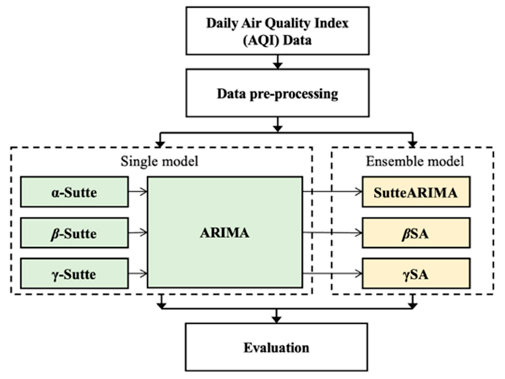
3. Materials and Methods

3.1. Data Collection

Data for this study were collected from the Daily Air Quality Index (AQI) data from the Environmental Information Open Platform of the Environmental Protection Department, Executive Yuan (https://data.epa.gov.tw/dataset/detail/AQX_P_434, accessed on 8 January 2022) [28]; the data were collected from January 2017 to December 2021, and the original data contained 11 variables, as shown in

Table 1. Dataset variable description.

Variable	Definition
siteid	station number
sitename	station name
monitordate	monitoring date
aqi	AQI Value
so2subindex	Sulfur dioxide sub-index
cosubindex	Carbon monoxide sub-index
o3subindex	Ozone sub-index
pm10subindex	suspended particulates sub-index
no2subindex	Nitrogen dioxide sub-index
o38subindex	Ozone 8-h sub-index
pm25subindex	fine suspended particulates sub-index

. Kumar & Goyal [29] pointed out that the change in air pollutant concentration emitted in the past can provide a reference for future air quality predictions. Therefore, the three variables“station name,” “monitoring date,” and AQI in the data set were used in this study.

3.2. The α-Sutte and Proposed γ-Sutte Indicator

Definitions and descriptions of notations in this study are shown in

Table 2. Notation of symbols.

Notation	Definition
$d\left(t\right)$	Observations at day $t$
$d\left(t-k\right)$	Observations at day $t-k$
$D_i$	The predicted value of day $i$
$\theta \left(t\right), \theta$	Observations on day $d\left(t-5\right)$
$\delta \left(t\right)$, $\delta$	Observations on day $d\left(t-4\right)$
$\alpha \left(t\right), \alpha$	Observations on day $d\left(t-3\right)$
$\beta \left(t\right), \beta$	Observations on day $d\left(t-2\right)$
$\gamma \left(t\right), \gamma$	Observations on day $d\left(t-1\right)$
$\Delta p\left(t\right), \Delta p$	$\delta \left(t\right)-\theta \left(t\right)$
$\Delta x\left(t\right), \Delta x$	$\alpha \left(t\right)-\delta \left(t\right)$
$\Delta y\left(t\right), \Delta y$	$\beta \left(t\right)-\alpha \left(t\right)$
$\Delta z\left(t\right), \Delta z$	$\gamma \left(t\right)-\beta \left(t\right)$
${\epsilon }_a\left(t\right), {\epsilon }_b\left(t\right), {\epsilon }_g\left(t\right)$	Error function
$w_a\left(t\right), w_b\left(t\right), w_g\left(t\right)$	Dynamic weighting function

.

The α-Sutte indicator was proposed in 2017, and can be used to predict a variety of different time series data [8]. During the forecasting process, the α-Sutte indicator only uses the previous four data points ($\gamma , \beta , \alpha , \delta$) to make a next-point forecast. It is therefore flexible when using any type of data [8]. The equation of the α-Sutte indicator is shown in Equation (1):

$$D_i=\frac{\alpha \left[\frac{\Delta x}{\frac{\alpha +\delta }{2}}\right]+\beta \left[\frac{\Delta y}{\frac{\beta +\alpha }{2}}\right]+\gamma \left[\frac{\Delta z}{\frac{\gamma +\beta }{2}}\right]}{3}$$

(1)

As can be seen in Equation (1), the α-Sutte indicator divides static weight, which is 1/3, into three different error items to make the final forecast. Although the β-Sutte indicator [9] uses dynamic weight to achieve a better result than the α-Sutte indicator, the sliding window size of β-Sutte indicator is 7 in calculating the dynamic weight. To reduce the computational cost further, the sliding window size of our new proposed γ-Sutte indicator is set to 5 in calculating dynamic weights. The equations of the proposed γ-Sutte indicator are shown in Equation (2).

$$D_i=w_a\left(t\right)·a\left(t\right)+w_b\left(t\right)·b\left(t\right)+w_g\left(t\right)·g\left(t\right)$$

(2)

where

$$a\left(t\right)=\left|\frac{\alpha \left(t\right)-\delta \left(t\right)}{\delta \left(t\right)}\right|, b\left(t\right)=\left|\frac{\beta \left(t\right)-\alpha \left(t\right)}{\alpha \left(t\right)}\right|, g\left(t\right)=\left|\frac{\gamma \left(t\right)-\beta \left(t\right)}{\beta \left(t\right)}\right|,c\left(t\right)=\left|\frac{\delta \left(t\right)-\theta \left(t\right)}{\theta \left(t\right)}\right|$$

(3)

and

$$w_a\left(t\right)=\frac{\frac{1}{{\epsilon }_a\left(t\right)}}{{{\displaystyle \sum }}_{j=1}^3\frac{1}{{\epsilon }_j\left(t\right)}}, w_b\left(t\right)=\frac{\frac{1}{{\epsilon }_b\left(t\right)}}{{{\displaystyle \sum }}_{j=1}^3\frac{1}{{\epsilon }_j\left(t\right)}} , w_g\left(t\right)=\frac{\frac{1}{{\epsilon }_g\left(t\right)}}{{{\displaystyle \sum }}_{j=1}^3\frac{1}{{\epsilon }_j\left(t\right)}}$$

(4)

where

$${\epsilon }_a\left(t\right)=\left|\alpha \left(t\right)-c\left(t\right)\right|, {\epsilon }_b\left(t\right)=\left|\alpha \left(t\right)-a\left(t\right)\right|, {\epsilon }_g\left(t\right)=\left|\alpha \left(t\right)-b\left(t\right)\right|$$

(5)

3.3. Overall Experimental Process

This section will introduce the overall experimental process of the single model and the ensemble model in detail. The overall experimental scenario is shown in Figure 1. The proposed γ-Sutte indicator was evaluated and compared with other single models and ensemble models. This study first carried out the prediction of a single time series model through the evaluation stage to compare different evaluation metrics to find the best prediction method. The ensemble model was also carried out according to a similar process. This study aims to establish whether a single time series model is sufficient to meet the prediction results in the prediction of AQI, or whether an ensemble model is needed to achieve a better prediction.

The experiment was divided into two stages. The first stage was the evaluation of a single time series model. The γ-Sutte indicator proposed in this study was compared with other methods (α-Sutte, β-Sutte, and ARIMA) using various evaluation metrics. Next was the evaluation stage of the ensemble model. Similar to the previous step, various evaluation metrics of the ensemble model (SutteARIMA, βSA, γSA) were compared.

3.3.1. Evaluation Process of Time Series Single Models

The evaluation process of the time series single models included data pre-processing, weight training, prediction of the α-Sutte indicator, the β-Sutte indicator, the γ-Sutte indicator, and ARIMA.

The detailed research process was as follows:

• Data pre-processing: To ensure the authenticity of the data, the negative value and outliers were removed during the preprocessing;
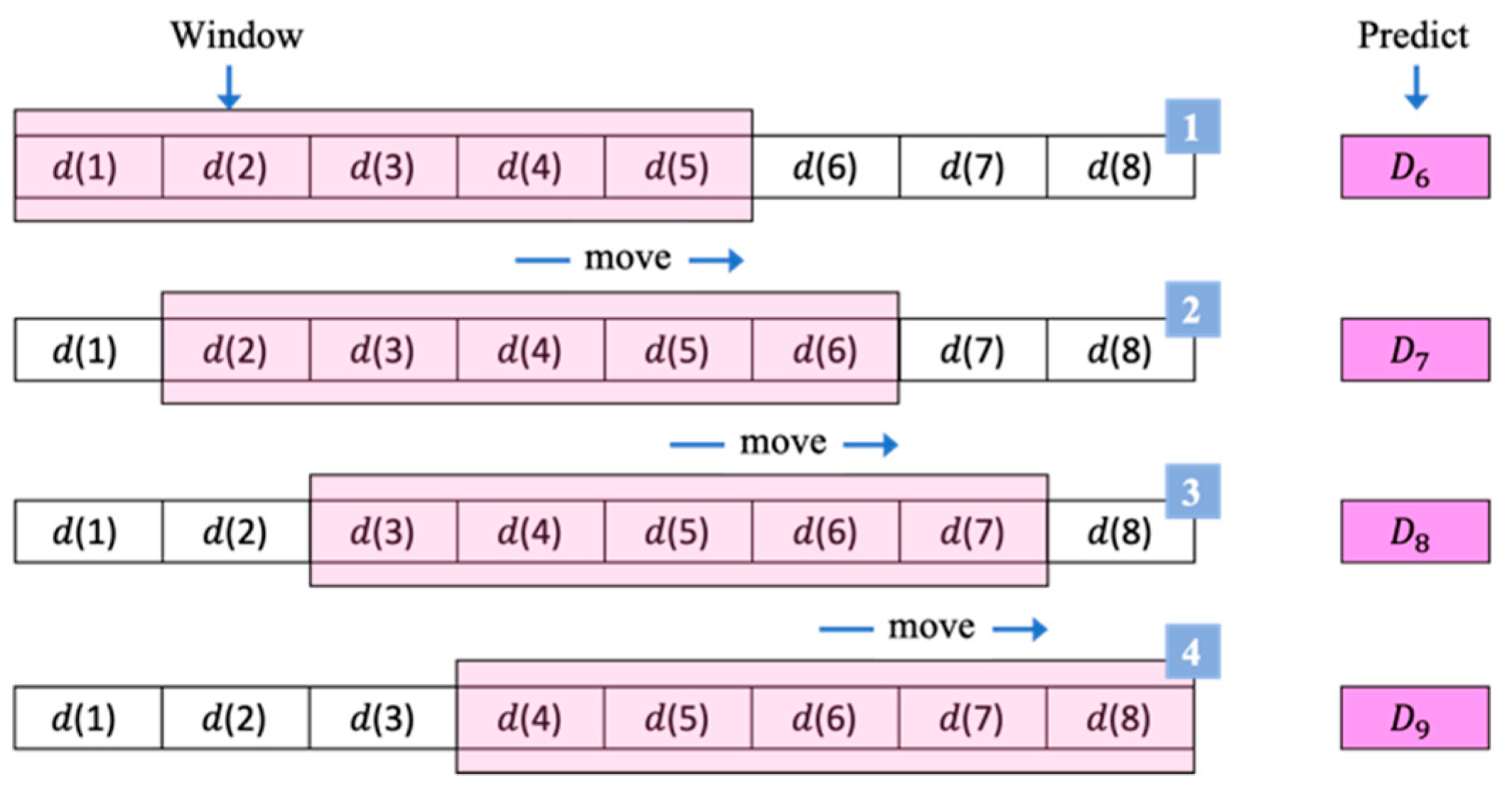
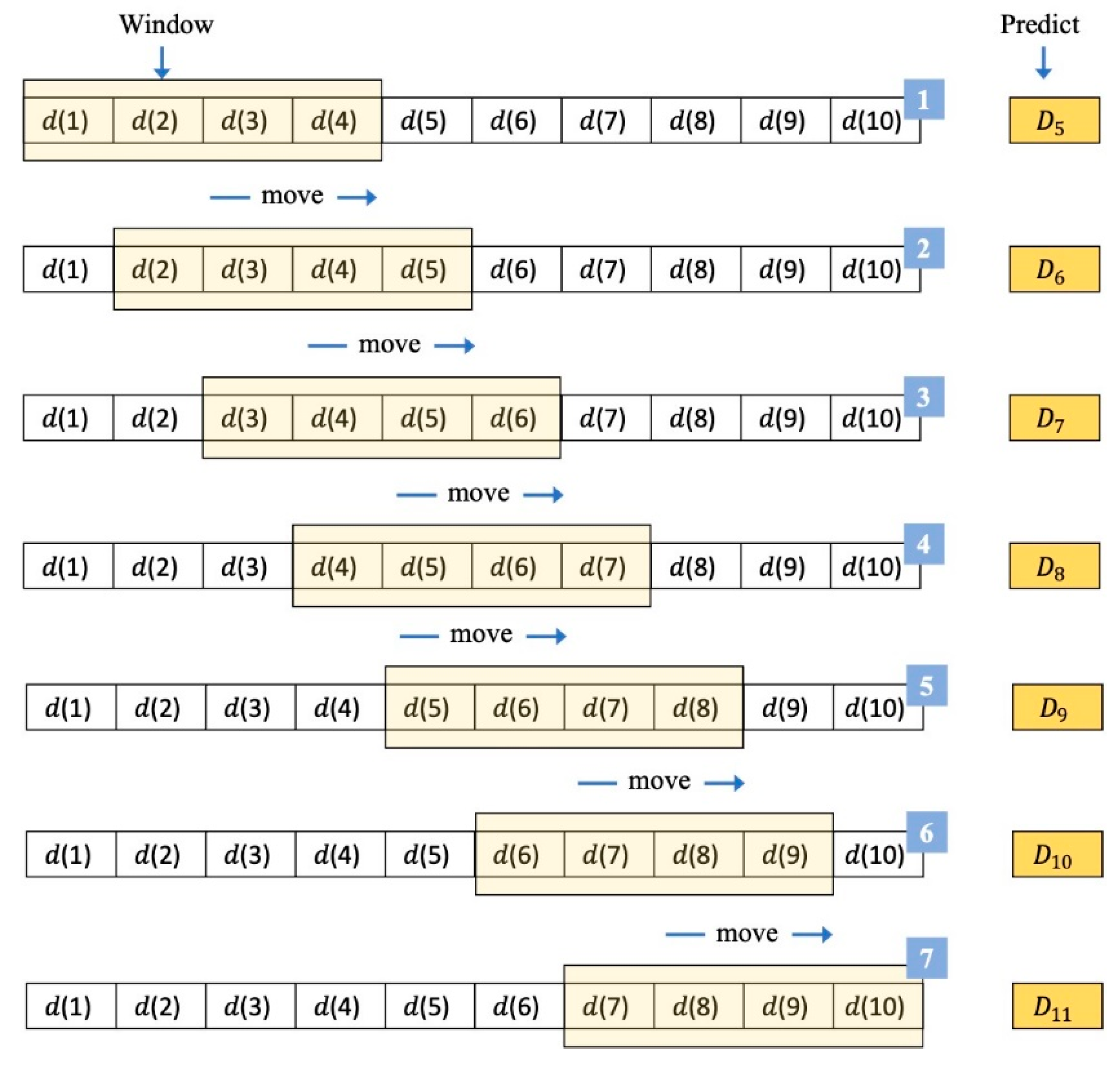
• The γ-Sutte indicator used a sliding window size of 5 to make the prediction as shown in Figure 2. For example, the γ-Sutte indicator used $d\left(1\right)$, $d\left(2\right)$, $d\left(3\right)$, $d\left(4\right)$, and $d\left(5\right)$ to predict $D_6$, then used $d\left(2\right)$, $d\left(3\right)$, $d\left(4\right)$, $d\left(5\right)$, and $d\left(6\right)$ to predict $D_7$, and so on;
• The sliding window size of the γ -Sutte indicator proposed in this study was set to 5, and took $d\left(1\right)$, $d\left(2\right)$, $d\left(3\right)$, $d\left(4\right)$, and $d\left(5\right)$, and used Equation (3) to calculate the variation of {$c\left(t\right)$, $a\left(t\right)$, $b\left(t\right)$, $g\left(t\right)$};
• After the calculation, three error values {${\epsilon }_a\left(t\right), {\epsilon }_b\left(t\right), {\epsilon }_g\left(t\right)$} of $c\left(t\right)$, $a\left(t\right)$, and $b\left(t\right)$ were calculated using Equation (5);
• The results from Step 4: ${\epsilon }_a\left(t\right), {\epsilon }_b\left(t\right), {\epsilon }_g\left(t\right)$ were adopted to Equation (4) to calculate the dynamic weights {$w_a\left(t\right), w_b\left(t\right), w_g\left(t\right)$};
• The weight obtained in Step 5 was put into Equation (2) to calculate the predicted value $D_6$;
• The four methods (α-Sutte indicator, β-Sutte indicator, γ-Sutte indicator, and ARIMA) of the time series single model were all evaluated using evaluation metrics.

3.3.2. The Evaluation Process of the Ensemble Models

The ensemble model evaluation process was divided into data preprocessing, weight training, SutteARIMA ensemble model prediction, βSA ensemble model prediction, γSA ensemble model prediction, and were evaluated by the chosen metrics.

The detailed evaluation process is described as follows:

• Data pre-processing: To ensure the authenticity of the data, the negative value and outliers were removed during the preprocessing;
• The ARIMA method used the same dataset, then averaged the results of the α-Sutte indicator and ARIMA, to become the final result of the SutteARIMA;
• The results of the other two methods, the β-Sutte indicator, and the γ-Sutte indicator, were averaged with the ARIMA results to form the results of the βSA, and the γSA ensemble models;
• The results of the three ensemble models were evaluated using the evaluation metrics.

3.4. Evaluation Metrics

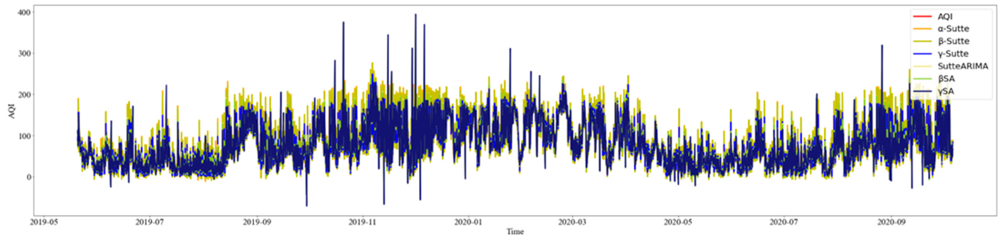
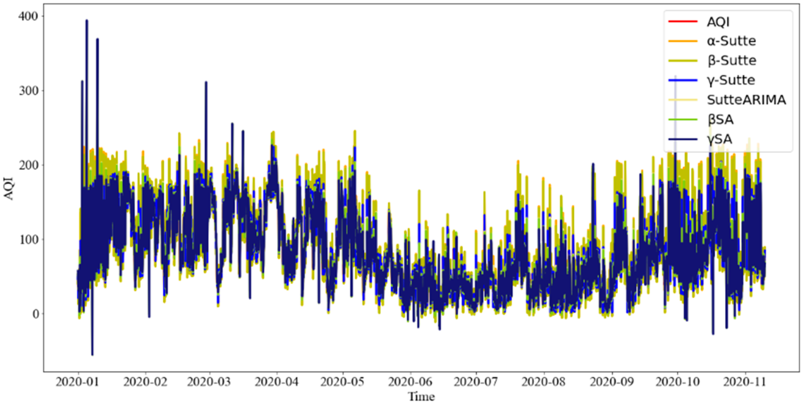
This study applied four general metrics in the evaluation, including mean absolute percentage error (MAPE), mean absolute error (MAE), root mean square error (RMSE), and coefficient of determination (R²). The smaller, the better for the first three indicators, and the bigger, the better for the last one.

The range of MAE and MAPE is from 0 to infinity. When the predicted value is completely consistent with the real value, MAE will be equal to 0; that is a perfect model. The greater the error, the greater the value of MAE. When MAPE is 0%, it means a perfect model; when MAPE is greater than 100%, it means an inferior model. The smaller the MAPE value is, the better accuracy the prediction model has. RMSE can measure the average difference between the predicted value and the actual value, and estimate the accuracy of the prediction model to predict the target value. The lower the RMSE value, the more accurate the prediction model [3]. R² ranges from 0 to 1. If R² = 0, it indicates that the model fit is poor; on the contrary, if R² = 1, the model fit is perfect. The larger the value is, the better the model fit is [30]. The forecast results of this study were obtained by using R, with the SutteForecastR package. Ahmar et al. [8] established the first α-Sutte indicator, using the stock price prediction of Turkish stocks as an experiment, and employed multiple forecasting methods (ARIMA, Regression, etc.) with MSE and RMSE as the evaluation metrics, and showed that the results of the α-Sutte indicator were the best. Therefore, this study also adopted the same methodology by using a different dynamic weighting function to evaluate the prediction results of the γ-Sutte indicator proposed.

4. Results

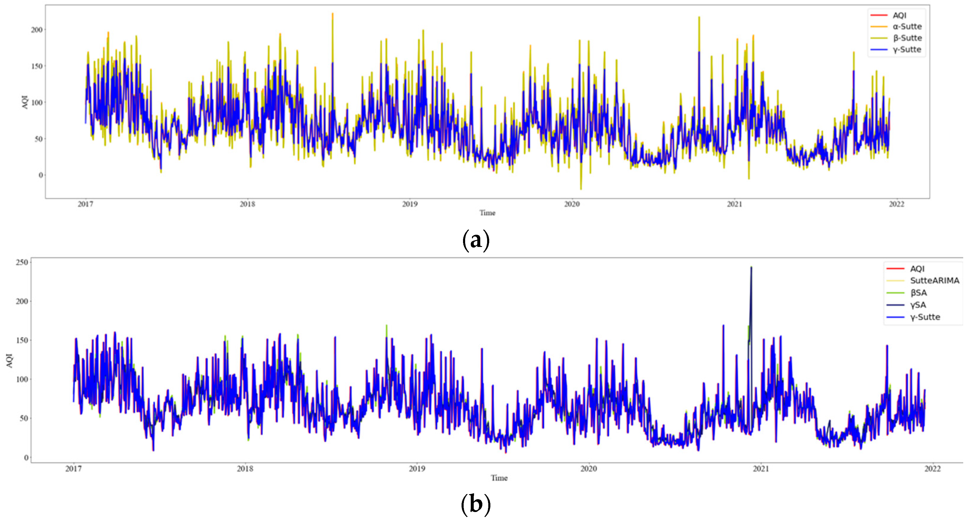
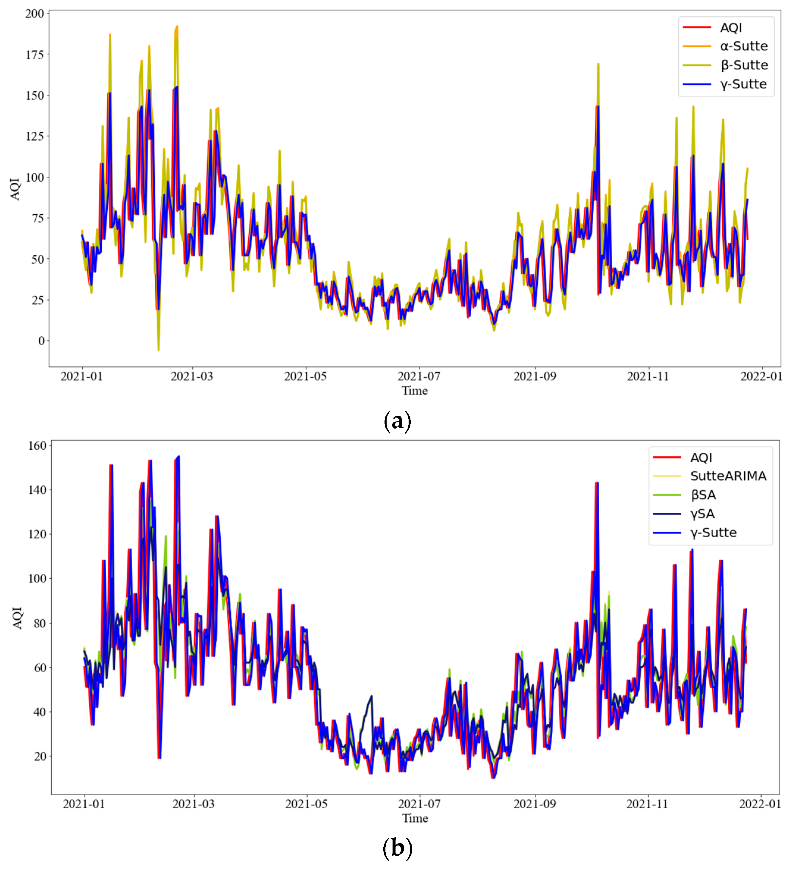
4.1. Time Series Single Model Evaluation

Four time series methods (the α-Sutte indicator, the β-Sutte indicator, the γ-Sutte indicator, and ARIMA) were evaluated for the prediction of the daily AQI for the No. 6 Naphtha Cracking Complex regions. The sliding window size of each method was different. The α-Sutte indicator was used to show the predicted values by the alpha.sutte() function of the sutteForecastR package in R. The β-Sutte indicator had the sliding window size set to 7, and the γ-Sutte indicator was set to 5. The ARIMA used the auto.arima() function in the FORECAST package in R to present the predicted value. Figure 3a shows the five-year prediction trend chart of the Naphtha Cracking Complex regions, both for the single time series and Figure 3b shows the five-year prediction trend chart for the ensemble model for comparison, where the X-axis is the year, and the Y-axis is the AQI value. According to the trend of the predicted value and the actual value in Figure 3, the rise and fall were very similar. However, and the pros and cons of the method could not be evaluated immediately. The time series model results predicting AQI daily over five years with the evaluation metrics are shown in

Table 3. Prediction results of the time series model in No. 6 Naphtha Cracking Complex region.

Evaluation Metrics	α-Sutte	β-Sutte	$\mathit{\gamma }$-Sutte	ARIMA
MAPE	35.52503	35.33326	28.15433	44.45941
MAE	20.40166	20.35359	16.3663	16.3663
RMSE	28.86724	28.69002	23.18071	34.22783
R2	0.4682005	0.4660149	0.5347211	0.1757319

.

Table 3 shows the comparisons of AQI prediction results (including ARIMA, the α-Sutte, the β-Sutte, and the γ-Sutte) daily in the No. 6 Naphtha Cracking Complex region in the past five years, as well as a variety of evaluation metrics (MAPE, MAE, RMSE, and R²); bold font represents the best evaluation result. The results showed that the γ-Sutte ranked at the top in all evaluation metrics.

4.2. Ensemble Model Evaluation

This study evaluated the prediction results of the three ensemble model methods (SutteARIMA, βSA, γSA) for the daily AQI of the No. 6 Naphtha Cracking Complex region. All methods used sliding windows, but the sliding window size of each method was different. The SutteARIMA first used the Auto.arima () function in the Forecast package of R to present ARIMA’s predicted value, then took the average value of the α-Sutte indicator and obtained the results of SutteARIMA. The βSA ensemble model was based on a sliding window size of 7, and the final result was the average of the β-Sutte indicator and ARIMA results. The sliding window size for the the γSA ensemble model was 5, and the final result was averaged by the γ-Sutte indicator and ARIMA results. Figure 4a shows the prediction trend chart of the ensemble models in 2021, for example; the single time series, in Figure 4b, is also shown for comparison. As it is difficult to see the difference from each trend chart, the prediction results of ensemble model in after the daily AQI in No. 6 Naphtha Cracking Complex region was evaluated using MAPE, MAE, RMSE, and R², which are shown in

Table 4. Results of the ensemble model in No. 6 Naphtha Cracking Complex regions.

Evaluation Metrics	SutteARIMA	βSA	$\mathit{\gamma }$SA	$\mathit{\gamma }$-Sutte
MAPE	32.60922	32.29693	32.1901	28.15433
MAE	17.25304	17.18177	17.10884	16.3663
RMSE	24.52663	24.45834	24.21541	23.18071
R2	0.4643722	0.4633891	0.4499986	0.5347211

.

Table 4 compares the ensemble model forecast results of the No. 6 Naphtha Cracking Complex regions over five years. This study has compared the proposed γ-Sutte indicator with other ensemble models (SutteARIMA, the βSA, the γSA) using specific evaluation metrics (MAPE, MAE, RMSE, R²). In Table 4, the bold font represents the best evaluation result. The proposed γ-Sutte had the best evaluation results in both the single time series model and the ensemble model.

5. Discussion

5.1. Transferable

“Transferable” refers to the fact that findings can be applied to objects or occasions other than the research context to understand people’s feelings about the same experience [31]. In order to verify that the method proposed for short-term AQI prediction can be applied to different datasets, Zhang et al. [7] showed in their study that the accuracy of the proposed method was the highest in any dataset, which also demonstrated its transferability. In order to verify the transferability of the proposed γ -Sutte indicator, four time series model methods (the α-Sutte indicator, the β-Sutte indicator, the γ-Sutte indicator, and ARIMA) and three ensemble model methods (SutteARIMA, the βSA, and the γSA) were applied to the AQI data of the Vientiane district, the capital city of Laos. The hourly AQI dataset for Vientiane is from the Air Quality data of the United States Consulate in Laos (https://www.airnow.gov/, accessed on 8 January 2022) [32] from January 2019 to December 2020; there are six variables in the original data. Three variables, “name of the station,” “date of monitoring,” and “air quality index,” are used in this study; the variables and definitions of the dataset are shown in

Table 5. Variables and definitions for the Vientiane area.

Variables	Definitions
Site	name of the station
Date.LT.	date of monitoring
AQI	air quality index
AQI.Category	Categories of air quality index
Raw.Conc.	-
QC.Name	-

.

Figure 5 shows the prediction trend of the two-year time series model and ensemble model in the Vientiane area of this study. The trend chart for 2020 is shown in Figure 6. The data preprocessing method and research process in the Vientiane area were the same as in the No. 6 Naphtha Cracking Complex region. The difference between the two is that the former predicts the AQI in days, while the latter predicts the AQI in hours. The comparison between the evaluation metrics of the other method is shown in

Table 6. Prediction results of time series model and ensemble model in the Vientiane area.

Evaluation Metrics	α-Sutte	β-Sutte	$\mathit{\gamma }$-Sutte	ARIMA	SutteARIMA	βSA	$\mathit{\gamma }$SA
MAPE	22.78845	22.61683	19.79801	63.85786	35.03214	34.90172	38.71741
MAE	10.90479	10.77376	9.059488	29.66419	15.5703	15.54959	17.72079
RMSE	16.08355	15.8108	13.76311	45.62253	23.58507	23.58148	26.33336
R2	0.9175967	0.9200563	0.9286815	0.4358475	0.7988707	0.7991491	0.7499707

.

Table 6 shows the evaluation results of predicting the AQI in the Vientiane area by hours in the past 2 years; The table shows the comparison of different evaluation metrics (MAPE, MAE, RMSE, and R²) in the single time series model (the α-SUtte, the β-Sutte, the γ-Sutte, and ARIMA) and the ensemble model (SutteARIMA, the βSA, and the γSA). The bold font represents the best evaluation result. The γ-Sutte was still the top method among all models. This study also found that the γ-Sutte indicator had good results for both day and hour predictions.

5.2. Discussion

In this study, the previous time series models (the α-Sutte indicator, the β-Sutte indicator, the γ-Sutte indicator, and ARIMA) and ensemble models (SutteARIMA, the βSA, and the γSA) were compared in their ability to predict the daily AQI of No. 6 Naphtha Cracking Complex region in Taiwan, and the hourly AQI of the Vientiane area in Laos. The results of these two different regions are shown in

Table 7. The prediction results of the time series and ensemble models in two regions.

Area	Metrics	α-Sutte	β-Sutte	$\mathit{\gamma }$-Sutte	ARIMA	SutteARIMA	βSA	$\mathit{\gamma }$SA
Mailiao	MAPE	35.52503	35.33326	28.15433	44.45941	32.60922	32.29693	32.1901
	MAE	20.40166	20.35359	16.3663	16.3663	17.25304	17.18177	17.10884
	RMSE	28.86724	28.69002	23.18071	34.22783	24.52663	24.45834	24.21541
	R2	0.4682005	0.4660149	0.5347211	0.1757319	0.4643722	0.4633891	0.4499986
Vientiane	MAPE	22.78845	22.61683	19.79801	63.85786	35.03214	34.90172	38.71741
	MAE	10.90479	10.77376	9.059488	29.66419	15.5703	15.54959	17.72079
	RMSE	16.08355	15.8108	13.76311	45.62253	23.58507	23.58148	26.33336
	R2	0.9175967	0.9200563	0.9286815	0.4358475	0.7988707	0.7991491	0.7499707

with the evaluation metrics (MAPE, MAE, RMSE, and R²). Bold font represents the best result across evaluations. The γ-Sutte indicator proposed in this study has the best prediction results compared to all others. It can be seen that the γ-Sutte indicator proposed in this study has good prediction performance in different regional datasets and different time segments. The results are discussed as follows:

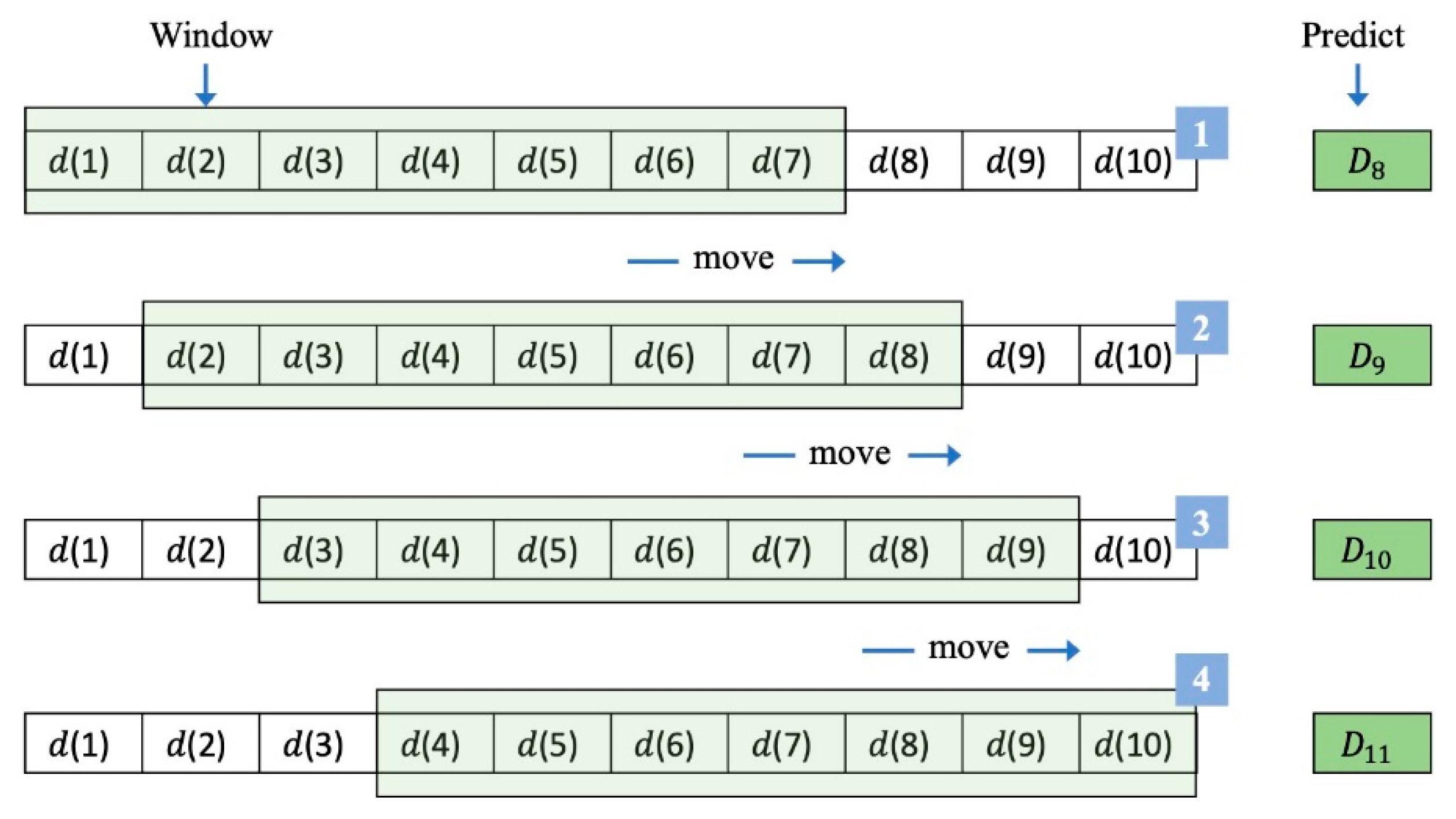
• The α-Sutte indicator [8] uses fixed weight, while the γ-Sutte indicator proposed in this study used dynamic weight to make predictions. The effect of dynamic weight on prediction was better than fixed weight because the weight was adjusted at all times according to the sliding window. Therefore, the prediction results of the β-Sutte indicator [9] in another study was also better than the α-Sutte indicator; this was verified in this study. Figure 7 and Figure 8 show the operation of the sliding window of the α-Sutte indicator and the β-Sutte indicator. Although the prediction results of the β-Sutte indicator were slightly better than that of the α-Sutte indicator, the required time window size was much larger than that of the α-Sutte indicator.
• The β-Sutte indicator [9] used the dynamic error weight and the sliding window size of 7 (in Figure 8), while the γ-Sutte indicator proposed in this study also used a different error dynamic weight to make predictions, with a sliding window size of only 5 (in Figure 3). In addition, the computational complexity of the α-Sutte indicator, the β-Sutte indicator, and the γ-Sutte indicator were O(1), O(2n), and O(n), respectively. The computational cost of the γ-Sutte indicator was relatively low compared to the β-sutte indicator. Nevertheless, the prediction results of the γ-Sutte indicator were better than the β-sutte indicator, indicating that the prediction results may be better if an appropriate error function and sliding window size are selected.
• Although the prediction results of the ARIMA model, which had a relatively high calculation time, was not better than that of the γ-Sutte indicator proposed in this study, the prediction results of ARIMA were still better than that of other time series models, indicating that the ARIMA prediction model is still feasible to use in time series analysis.
• Traditionally, the prediction results of the ensemble model were better than those of the single model. However, if the prediction results of the single model selected are not very good, then they will weaken the advantages of the ensemble model; this was verified in the experiment of this study.

6. Conclusions

Ahmar et al. [8] proposed the α-Sutte indicator based on time series analysis, which was shown to be excellent in time series prediction; however, the calculation of the α-Sutte indicator uses fixed weights. Shih et al. [9] proposed another more accurate β-Sutte indicator which used dynamic weight. However, the computational complexity and sliding window required of the β-Sutte indicator were still too high when compared with the α-Sutte indicator. Therefore, a modified γ-Sutte indicator to reduce the computational time and complexity of the β-Sutte indicator was proposed in this study. The computational complexity of the α-Sutte indicator, the β-Sutte indicator, and the γ-Sutte indicator were O(1), O(2n), and O(n), respectively. The computational cost of the γ-Sutte indicator was relatively low compared to the β-sutte indicator. Nevertheless, the prediction results of the γ-Sutte indicator were better than both the α-Sutte indicator and the β-sutte indicator. The γ-Sutte indicator only used the data of the previous five days to make predictions, and the computational cost was less than the β-Sutte indicator. The final results showed that the evaluation metrics of the γ -Sutte indicator (MAPE, MAE, RMSE, and R²) were better than those of the other six methods (the α-Sutte indicator, the β-Sutte indicator, ARIMA, SutteARIMA, the βSA, and the γSA) in all areas. In addition, this study also proved the transferability of the γ-Sutte indicator as an air quality predictor in the Vientiane area. Therefore, the γ-Sutte indicator is an effective air quality prediction indicator.

This study has the following limitations and recommendations for the future:

• To calculate dynamic weight, the training calculation time of the γ-Sutte indicator proposed in this study was higher than that of the α-Sutte indicator which uses a fixed weight. The calculation cost was lower than that of the β-Sutte indicator with dynamic weight. However, the prediction results of the γ-Sutte indicator was among the best. Nevertheless, if the prediction results are arbitrary and with acceptable accuracy, the α-Sutte indicators may be the best option.
• In addition to the daily AQI prediction in the Mailiao district, this study also conducted the hourly AQI prediction experiment in the Vientiane district. The results showed that the γ-Sutte Indicator also had good prediction ability in different periods, representing this method’s transferability and generalization.
• The main reason why the modified γ-Sutte indicator was proposed is that although the prediction abilities of the β-Sutte indicator established by Shih [9] were slightly better than those of the α-Sutte indicator, the calculation cost was higher than that of α-Sutte. Therefore, this study proposed a more efficient modified γ-Sutte indicator.
• In the prediction of AQI, other variables should be considered in the future, such as wind direction, nearby stations, climate, etc.
• For the ensemble model, combinations of the γ-Sutte indicator with other time series methods in the future to form a better model should be explored, such as the Holt-Winters Model.
• In addition, perhaps deep learning and artificial neural networks can be compared together in the future. Wang [33] proposed an optimized echo state network for effective time series prediction. Compared with other artificial neural networks, the most apparent advantage of echo state network (ESN) is its more straightforward network structure and lower computational cost. Two real-time series datasets were used for prediction experiments, and the experimental results of the optimized ESN were also quite excellent. Xu [34] proposed multi-variable LSTM (MV-LSTM) to better capture the different temporal dynamics of multivariate sequences in an interpretable form. This model dramatically improves the prediction model’s performance and has a good effect on the housing load prediction. By evaluating each variable’s contribution to the prediction, the multi-quantile prediction of multiple time steps in the future can be generated.

References

1. World Health Organization. Ambient (Outdoor) Air Quality and Health, Fact Sheet No. 313. Available online: http://www.who.int/mediacentre/factsheets/fs313/en/ (accessed on 1 August 2022).
2. International Agency for Research on Cancer (IARC). Outdoor Air Pollution. In IARC Monographs on the Evaluation of Carcinogenic Risks to Humans; International Agency for Research on Cancer: Lyon, France, 2013; Volume 109. [Google Scholar]
3. Zhu, S.; Lian, X.; Liu, H.; Hu, J.; Wang, Y.; Che, J. Daily air quality index forecasting with hybrid models: A case in China. Environ. Pollut. 2017, 231, 1232–1244. [Google Scholar] [CrossRef]
4. Wu, Q.; Lin, H. A novel optimal-hybrid model for daily air quality index prediction considering air pollutant factors. Sci. Total Environ. 2019, 683, 808–821. [Google Scholar] [CrossRef]
5. Wang, J.; Li, J.; Wang, X.; Wang, J.; Huang, M. Air quality prediction using CT-LSTM. Neural Comput. Appl. 2021, 33, 4779–4792. [Google Scholar] [CrossRef]
6. Han, Y.; Li, V.O.; Lam, J.C.; Pollitt, M. How BLUE is the sky? Estimating air qualities in Beijing during the Blue-Sky Day period (2008–2012) by Bayesian multi-task LSTM. Environ. Sci. Policy 2021, 116, 69–77. [Google Scholar] [CrossRef]
7. Zhang, L.; Na, J.; Zhu, J.; Shi, Z.; Zou, C.; Yang, L. Spatiotemporal causal convolutional network for forecasting hourly PM2.5 concentrations in Beijing, China. Comput. Geosci. 2021, 155, 104869. [Google Scholar] [CrossRef]
8. Ahmar, A.S.; Rahman, A.; Mulbar, U. Implementation of α-Sutte Indicator to Forecasting Consumer Price Index in Turkey. In Proceedings of the International Conference On Mathematics and Natural Sciences, Bali, Indonesia, 6–7 September 2017; pp. 1–4. [Google Scholar]
9. Shih, D.-H.; Wu, T.-W.; Shih, M.-H.; Yang, M.-J.; Yen, D.C. A Novel βSA Ensemble Model for Forecasting the Number of Confirmed COVID-19 Cases in the US. Mathematics 2022, 10, 824. [Google Scholar] [CrossRef]
10. Cheng, W.-L.; Chen, Y.-S.; Zhang, J.; Lyons, T.; Pai, J.-L.; Chang, S.-H. Comparison of the revised air quality index with the PSI and AQI indices. Sci. Total Environ. 2007, 382, 191–198. [Google Scholar] [CrossRef]
11. Benchrif, A.; Wheida, A.; Tahri, M.; Shubbar, R.M.; Biswas, B. Air quality during three covid-19 lockdown phases: AQI, PM2.5 and NO2 assessment in cities with more than 1 million inhabitants. Sustain. Cities Soc. 2021, 74, 103170. [Google Scholar] [CrossRef]
12. Li, Y.; Chiu, Y.-h.; Lu, L.C. Energy and AQI performance of 31 cities in China. Energy Policy 2018, 122, 194–202. [Google Scholar] [CrossRef]
13. Ren, Y.-S.; Narayan, S.; Ma, C.-q. Air quality, COVID-19, and the oil market: Evidence from China’s provinces. Econ. Anal. Policy 2021, 72, 58–72. [Google Scholar] [CrossRef]
14. Li, X.; Hu, Z.; Cao, J.; Xu, X. The impact of environmental accountability on air pollution: A public attention perspective. Energy Policy 2022, 161, 112733. [Google Scholar] [CrossRef]
15. Sethi, J.K.; Mittal, M. Analysis of air quality using univariate and multivariate time series models. In Proceedings of the 2020 10th International Conference on Cloud Computing, Data Science & Engineering (Confluence), Noida, India, 29–31 January 2020. [Google Scholar]
16. Phruksahiran, N. Improvement of air quality index prediction using geographically weighted predictor methodology. Urban Clim. 2021, 38, 100890. [Google Scholar] [CrossRef]
17. Yan, R.; Liao, J.; Yang, J.; Sun, W.; Nong, M.; Li, F. Multi-hour and multi-site air quality index forecasting in Beijing using CNN, LSTM, CNN-LSTM, and spatiotemporal clustering. Expert Syst. Appl. 2021, 169, 114513. [Google Scholar] [CrossRef]
18. Liu, H.; Yan, G.; Duan, Z.; Chen, C. Intelligent modeling strategies for forecasting air quality time series: A review. Appl. Soft Comput. 2021, 102, 106957. [Google Scholar] [CrossRef]
19. Ahmar, A.S. Sutte Indicator: A technical indicator in stock market. Int. J. Econ. Financ. Issues 2017, 7, 223–226. [Google Scholar]
20. Ahmar, A.S. A comparison of α-Sutte Indicator and ARIMA methods in renewable energy forecasting in Indonesia. Int. J. Eng. Technol. 2018, 7, 20–22. [Google Scholar] [CrossRef]
21. Lippi, M.; Bertini, M.; Frasconi, P. Short-term traffic flow forecasting: An experimental comparison of time-series analysis and supervised learning. IEEE Trans. Intell. Transp. Syst. 2013, 14, 871–882. [Google Scholar] [CrossRef]
22. Rekhi, J.K.; Nagrath, P.; Jain, R. Forecasting Air Quality of Delhi Using ARIMA Model. In Advances in Data Sciences, Security and Applications; Springer: Berlin/Heidelberg, Germany, 2020; pp. 315–325. [Google Scholar]
23. Aladağ, E. Forecasting of particulate matter with a hybrid ARIMA model based on wavelet transformation and seasonal adjustment. Urban Clim. 2021, 39, 100930. [Google Scholar] [CrossRef]
24. Gopu, P.; Panda, R.R.; Nagwani, N.K. Time Series Analysis Using ARIMA Model for Air Pollution Prediction in Hyderabad City of India. In Soft Computing and Signal Processing; Springer: Berlin/Heidelberg, Germany, 2021; pp. 47–56. [Google Scholar]
25. Li, Y.; Pan, Y. A novel ensemble deep learning model for stock prediction based on stock prices and news. Int. J. Data Sci. Anal. 2022, 13, 139–149. [Google Scholar] [CrossRef]
26. Ahmar, A.S.; Del Val, E.B. SutteARIMA: Short-term forecasting method, a case: COVID-19 and stock market in Spain. Sci. Total Environ. 2020, 729, 138883. [Google Scholar] [CrossRef]
27. Ejohwomu, O.A.; Shamsideen Oshodi, O.; Oladokun, M.; Bukoye, O.T.; Emekwuru, N.; Sotunbo, A.; Adenuga, O. Modelling and Forecasting Temporal PM2.5 Concentration Using Ensemble Machine Learning Methods. Buildings 2022, 12, 46. [Google Scholar] [CrossRef]
28. Executive Yuan. Environmental Information Open Platform of the Environmental Protection Department. Available online: https://data.epa.gov.tw/dataset/detail/AQX_P_434 (accessed on 8 January 2022).
29. Kumar, A.; Goyal, P. Forecasting of daily air quality index in Delhi. Sci. Total Environ. 2011, 409, 5517–5523. [Google Scholar] [CrossRef] [PubMed]
30. Shahid, N.; Shah, M.A.; Khan, A.; Maple, C.; Jeon, G. Towards Greener Smart Cities and Road Traffic Forecasting Using Air Pollution Data. Sustain. Cities Soc. 2021, 72, 103062. [Google Scholar] [CrossRef]
31. Korstjens, I.; Moser, A. Series: Practical guidance to qualitative research. Part 4: Trustworthiness and publishing. Eur. J. Gen. Pract. 2018, 24, 120–124. [Google Scholar] [CrossRef]
32. Air Quality Data of the United States Consulate in Laos. Available online: https://www.airnow.gov/ (accessed on 8 January 2022).
33. Wang, Z.; Zeng, Y.R.; Wang, S.; Wang, L. Optimizing echo state network with backtracking search optimization algorithm for time series forecasting. Eng. Appl. Artif. Intell. 2019, 81, 117–132. [Google Scholar] [CrossRef]
34. Xu, C.; Li, C.; Zhou, X. Interpretable LSTM Based on Mixture Attention Mechanism for Multi-Step Residential Load Forecasting. Electronics 2022, 11, 2189. [Google Scholar] [CrossRef]
Figure 1. The overall experimental scenario.
Mathematics 10 03060 g001
Figure 2. Sliding window of the γ-Sutte indicator.
Mathematics 10 03060 g002
Figure 3. Five-year prediction chart of No. 6 Naphtha Cracking Complex regions. (a) Time series model; (b) Ensemble model.
Mathematics 10 03060 g003
Figure 4. 2021 prediction chart of No. 6 Naphtha Cracking Complex regions. (a) Ensemble model; (b) Single time series.
Mathematics 10 03060 g004
Figure 5. Two-year trend chart of the time series model and ensemble model in the Vientiane area.
Mathematics 10 03060 g005
Figure 6. Time series model and ensemble model trend chart of the Vientiane area in 2020.
Mathematics 10 03060 g006
Figure 7. Sliding window of the α-Sutte indicator.
Mathematics 10 03060 g007
Figure 8. Sliding window of the β-Sutte indicator.
Mathematics 10 03060 g008