Theoretical Study on Non-Improvement of the Multi-Frequency Direct Sampling Method in Inverse Scattering Problems

Abstract

Generally, it has been confirmed that applying multiple frequencies guarantees a successful imaging result for various non-iterative imaging algorithms in inverse scattering problems. However, the application of multiple frequencies does not yield good results for direct sampling methods (DSMs), which has been confirmed through simulation but not theoretically. This study proves this premise theoretically by showing that the indicator function with multi-frequency can be expressed by the Bessel and Struve functions and the propagation direction of the incident field. This is based on the fact that the indicator function with single frequency can be expressed by the exponential and Bessel function of order zero of the first kind. Various simulation outcomes are shown to support the theoretical result.

1. Introduction

The direct sampling method (DSM) is a sampling-type, non-iterative technique for retrieving unknown scatterers’ location and/or shape. It was first introduced for 2D inverse medium scattering for fixed plane incident waves [1], and it was subsequently applied and extended to various inverse problems, including identifying 2D and 3D electromagnetic inhomogeneities [2,3,4,5], electrical impedance tomography [6], diffusive optical tomography [7], inhomogeneity detection in mono-static [8] measurement configurations, source detection in stratified ocean waveguide [9,10], localizing short, linear, and perfectly conducting cracks [11], retrieving magnetic inhomogeneity locations in transverse electric (TE) polarization [12], anomaly detection in microwave imaging [13], phaseless inverse source scattering [14], and real-world microwave imaging [15]. We reference various studies [16,17] related to the direct sampling method.

Generally, DSM is a fast scheme because it does not require additional operations (e.g., singular-value decomposition, generating additional operators, solving ill-posed integral equations or adjoint problems, etc.), and it is robust with respect to random noise. Although DSM requires only a few (one or two) incident waves to identifying unknown target locations, image quality is generally poorer than other techniques that use several incident waves, such as Kirchhoff/subspace migrations, MUltiple SIgnal Classification (MUSIC), and the linear sampling method. Therefore, it is natural to consider improvements for traditional DSM.

Applying multiple frequencies is a promising method to help obtain good results for many non-iterative techniques in various inverse scattering problems. Previous studies regarding multi-frequency imaging have investigated many non-iterative methods and successfully applied the approach to subspace migration [18,19], the linear sampling method [20,21], topological derivatives [22,23], MUSIC [24,25], etc. However, it is difficult to obtain good results from applying traditional multi-frequency methods for DSM and the orthogonality sampling method (OSM) with a fixed single incident field. Almost every small target can be identified using single-frequency DSM or OSM, but only few specific targets can be recognized using multi-frequency DSM or OSM. Many numerical simulations have confirmed that detection is significantly dependent on the propagation direction [1,26,27], but the underlying theoretical basis for this non-improvement for multi-frequency compared with single-frequency DSM or OSM has not been confirmed. Therefore, this paper establishes a mathematical theory to explain multi-frequency DSM non-improvement.

This study analyzed the DSM multi-frequency indicator function structure with a fixed incident field to identify a set of short, well-separated, linear, and perfectly conducted cracks for the full-aperture inverse scattering problem. We first established a relationship with combined Bessel and Struve functions of order zero and one as well as the plane-wave incident field propagation direction, since the single-frequency DSM indicator function can be expressed by the exponential and Bessel function of order zero of the first kind. Based on the analyzed structure, we examine certain multi-frequency DSM properties and why only few targets can be recognized and recognition is significantly dependent on the incident field direction.

The remainder of this paper is organized as follows. Section 2 briefly introduces 2D direct scattering in the presence of small cracks and the DSM single and multi-frequency indicator function. Section 3 presents qualitative analysis regarding the DSM multi-frequency indicator function structure and discusses intrinsic multi-frequency DSM properties. Section 4 presents numerical simulation results to support the theoretical result. Section 5 summarizes and concludes the paper.

Finally, let us mention that in connection with the current contribution about the full-aperture inverse scattering problem, we refer the reader to [28,29,30] as remarkable references indicating that the application of multiple frequencies is essential for obtaining good results in the limited-aperture inverse scattering problem.

2. Two-Dimensional Direct Scattering Problem and the Indicator Function of OSM

In this section, we briefly survey the two-dimensional direct scattering problem in the existence of perfectly conducting cracks. Throughout this paper, we denote ${\mathrm{\Gamma }}_m$ as a linear crack with a small length $2{\ell }_m$ centered at ${\mathbf{r}}_m$, $m=1,2,\cdots ,M$, and they are well-separated from each other. For that sake, we let $\mathrm{\Gamma }$ be the collection of all ${\mathrm{\Gamma }}_m$ and assume the length of all cracks to be the same i.e., ${\ell }_m=\ell$ for all m.

Let $u_{inc}(\mathbf{x},\mathbf{d})=e^{ik\mathbf{d}·\mathbf{x}}$ be the given incident plane-wave with a fixed propagation direction $\mathbf{d}\in {\mathbb{S}}^1$, where ${\mathbb{S}}^1$ denotes the two-dimensional unit circle centered at the origin, and $u_{tot}(\mathbf{x},\mathbf{d})$ denotes the total field that satisfies the following Helmholtz equation

$$▵u_{tot}(\mathbf{x},\mathbf{d})+k^2{u}_{tot}(\mathbf{x},\mathbf{d})=0\mathrm{in}{\mathbb{R}}^2\setminus \overline{\mathrm{\Gamma }}$$

(1)

with Dirichlet boundary condition

$$u_{tot}(\mathbf{x},\mathbf{d})=0\mathrm{on}\mathrm{\Gamma }.$$

(2)

here, $k=2\pi /\lambda$ denotes the background wavenumber that satisfies $4k|{\mathbf{r}}_m-{\mathbf{r}}_{m^{\prime }}|\gg 1$ for $m\ne m^{\prime }$, while $\lambda$ is the given wavelength. Since each ${\mathrm{\Gamma }}_m$ is a small crack, we assume that ℓ is small enough such that $2\ell \ll \lambda$.

Let $u_{scat}(\mathbf{x},\mathbf{d})=u_{tot}(\mathbf{x},\mathbf{d})-u_{inc}(\mathbf{x},\mathbf{d})$ be the scattered field corresponding to the incident field $u_{inc}(\mathbf{x},\mathbf{d})$ that satisfies the Sommerfeld radiation condition. The far-field pattern $u_{\infty }(\theta ,\mathbf{d})$ of scattered field $u_{scat}(\mathbf{x},\mathbf{d})$ is given by the following relation

$$u_{scat}(\mathbf{x},\mathbf{d})=\frac{e^{ik\left|\mathbf{x}\right|}}{\sqrt{\left|\mathbf{x}\right|}}\left\{u_{\infty }(\theta ,\mathbf{d})+\mathcal{O}\left(\frac{1}{\left|\mathbf{x}\right|}\right)\right\},\left|\mathbf{x}\right|⟶+\infty$$

uniformly in all the directions $\theta =\mathbf{x}/\left|\mathbf{x}\right|$. Note that $u_{\infty }(\theta ,\mathbf{d})$ can be represented as the single-layer potential with unknown density function $\phi (\mathbf{r},\mathbf{d})$:

$$u_{\infty }(\theta ,\mathbf{d})=-\frac{1+i}{4\sqrt{\pi k}}\sum _{m=1}^M{\int }_{{\mathrm{\Gamma }}_m}{e}^{-ik\theta ·\mathbf{r}}{\phi }_m(\mathbf{r},\mathbf{d})d\mathbf{r}.$$

(3)

Based on [31], the densify function ${\phi }_m$ is assumed to be of the form

$${\phi }_m(\mathbf{r},\mathbf{d})=\frac{{\tilde{\phi }}_m(\mathbf{r},\mathbf{d})}{\sqrt{|\mathbf{r}-{\mathbf{e}}_{m,1}\left|\right|\mathbf{r}-{\mathbf{e}}_{m,2}|}},\mathbf{r}\in \mathrm{\Gamma }\setminus \bigcup _{m=1}^M\left\{{\mathbf{e}}_{m,1},{\mathbf{e}}_{m,2}\right\},$$

where ${\tilde{\phi }}_m\in \mathcal{C}\left({\mathrm{\Gamma }}_m\right)$, ${\mathbf{e}}_{m,1}$ and ${\mathbf{e}}_{m,2}$ denote the end-points of ${\mathrm{\Gamma }}_m$, $m=1,2,\cdots ,M$.

Now, let us denote ${\mathbf{V}}_{meas}\left(k\right)$ as the arrangement of the far-field pattern data with several directions ${\theta }_n$, $n=1,2,\cdots ,N$ at given wavenumber k such that

$${\mathbf{V}}_{meas}\left(k\right)=\left(u_{\infty }({\theta }_1,\mathbf{d}),u_{\infty }({\theta }_2,\mathbf{d}),\cdots ,u_{\infty }({\theta }_N,\mathbf{d})\right),$$

where the observation directions ${\theta }_n$ are distributed uniformly on ${\mathbb{S}}^1$ such that

$${\theta }_n=\left(cos\frac{2n\pi }{N},sin\frac{2n\pi }{N}\right).$$

Since the complete form of the density function $\phi$ of (3) is unknown, it is hard to directly design the indicator function of the DSM. Instead, we apply the asymptotic expansion formula, which is derived in [32].

Lemma 1

(Asymptotic Expansion Formula). Let $u_{tot}(\mathbf{x},\mathbf{d})$ satisfy (1) and (2). Then, for $0<2\ell \ll \lambda$, the following asymptotic expansion formula holds

$$u_{\infty }(\theta ,\mathbf{d})=-\frac{(1+i)\sqrt{\pi }}{\sqrt{4k}ln(\ell /2)}\sum _{m=1}^M{e}^{ik(\mathbf{d}-\theta )·{\mathbf{r}}_m}+\mathcal{O}\left(\frac{1}{{|ln\ell |}^2}\right).$$

(4)

In view of expansion (4), we can examine the structure of ${\mathbf{V}}_{meas}\left(k\right)$ as

$${\mathbf{V}}_{meas}\left(k\right)\approx -\frac{(1+i)\sqrt{\pi }}{\sqrt{4k}ln(\ell /2)}\sum _{m=1}^M{e}^{ik\mathbf{d}·{\mathbf{r}}_m}\left(e^{-ik{\theta }_1·{\mathbf{r}}_m},e^{-ik{\theta }_2·{\mathbf{r}}_m},\cdots ,e^{-ik{\theta }_N·{\mathbf{r}}_m}\right).$$

Thus, to extract ${\mathbf{r}}_m$ from ${\mathbf{V}}_{meas}\left(k\right)$, it is natural to examine the orthonormality between ${\mathbf{V}}_{meas}\left(k\right)$ and the following test vector

$${\mathbf{V}}_{test}(\mathbf{x},k)=\left(e^{-ik{\theta }_1·\mathbf{x}},e^{-ik{\theta }_2·\mathbf{x}},\cdots ,e^{-ik{\theta }_N·\mathbf{x}}\right).$$

With this, the indicator function ${\mathfrak{F}}_{DSM}(\mathbf{x},k)$ at k can be introduced as follows

$${\mathfrak{F}}_{DSM}(\mathbf{x},k)=\left|\frac{{\mathbf{V}}_{meas}\left(k\right)}{|{\mathbf{V}}_{meas}\left(k\right)|}·\frac{{\overline{\mathbf{V}}}_{test}(\mathbf{x},k)}{|{\overline{\mathbf{V}}}_{test}(\mathbf{x},k)|}\right|=\frac{|\langle u_{\infty }({\theta }_n,\mathbf{d}),e^{-ik{\theta }_n·\mathbf{x}}\rangle |}{\parallel u_{\infty }({\theta }_n,\mathbf{d}){\parallel }_{L^2\left({\mathbb{S}}^1\right)}{\parallel e^{-ik{\theta }_n·\mathbf{x}}\parallel }_{L^2\left({\mathbb{S}}^1\right)}},$$

where

$$\begin{array}{cc}\hfill & \langle u_{\infty }({\theta }_n,\mathbf{d}),e^{-ik{\theta }_n·\mathbf{x}}\rangle =\sum _{n=1}^N{u}_{\infty }({\theta }_n,\mathbf{d})\overline{e^{-ik{\theta }_n·\mathbf{x}}}\approx {\int }_{{\mathbb{S}}^1}{u}_{\infty }(\theta ,\mathbf{d})e^{-ik\theta ·\mathbf{x}}d\theta \hfill \end{array}$$

and

$$\begin{array}{c}\parallel u_{\infty }({\theta }_n,\mathbf{d}){\parallel }_{L^2\left({\mathbb{S}}^1\right)}={\left(\langle u_{\infty }({\theta }_n,\mathbf{d}),e^{-ik{\theta }_n·\mathbf{x}}\rangle \right)}^{1/2}.\hfill \end{array}$$

Then, ${\mathfrak{F}}_{DSM}(\mathbf{x},k)\approx 1$ when $\mathbf{x}={\mathbf{r}}_m$ whereas $0\le {\mathfrak{F}}_{DSM}(\mathbf{x},k)<1$ when $\mathbf{x}\ne {\mathbf{r}}_m$ for $m=1,2,\cdots ,M$. We refer to [3] for a detailed description of the indicator function.

Now, we introduce the following general multi-frequency indicator function (see [18] for instance): for several wavenumbers $k_f$, $f=1,2,\cdots ,F$,

$$\begin{array}{c}\hfill \begin{array}{cc}\hfill {\mathfrak{F}}_{MDSM}(\mathbf{x},k_1,k_F,F)& =\frac{1}{F}\left|\sum _{f=1}^F\frac{{\mathbf{V}}_{meas}\left(k_f\right)}{|{\mathbf{V}}_{meas}\left(k_f\right)|}·\frac{{\overline{\mathbf{V}}}_{test}(\mathbf{x},k_f)}{|{\overline{\mathbf{V}}}_{test}(\mathbf{x},k_f)|}\right|\hfill \\ \hfill & =\frac{1}{F}\left|\sum _{f=1}^F\frac{\langle u_{\infty }({\theta }_n,\mathbf{d}),e^{-i{k}_f{\theta }_n·\mathbf{x}}\rangle }{\parallel u_{\infty }({\theta }_n,\mathbf{d}){\parallel }_{L^2\left({\mathbb{S}}^1\right)}{\parallel e^{-i{k}_f{\theta }_n·\mathbf{x}}\parallel }_{L^2\left({\mathbb{S}}^1\right)}}\right|.\hfill \end{array}\end{array}$$

(5)

here, the wavenumbers $k_f$ are assumed to be equidistributed in the interval $[k_1,k_F]$. Notice that in contrast to the general multi-frequency imaging, the result obtained by the ${\mathfrak{F}}_{MDSM}(\mathbf{x},k_1,k_F,F)$ is worse than the one via the ${\mathfrak{F}}_{DSM}(\mathbf{x},k)$. This fact has been examined through the simulation results (see ([27], Section 3.2) for a related discussion), but the theoretical reason has not been satisfactorily established.

Remark 1

(Different type of indicator functions). Since, in some times, the indicator function ${\mathfrak{F}}_{MDSM}(\mathbf{x},k_1,k_F,F)$ does not guarantee good results, various multi-frequency indicator functions have been proposed. For example, in ([27], Section 3.2),

$${\mathfrak{F}}_{MF}(\mathbf{x},k_1,k_F,F)=\sum _{f=1}^F|{\mathbf{V}}_{meas}\left(k\right)·{\overline{\mathbf{V}}}_{test}(\mathbf{x},k){|}^p=\sum _{f=1}^F|\langle u_{\infty }({\theta }_n,\mathbf{d}),e^{-ik{\theta }_n·\mathbf{x}}\rangle {|}^p$$

(6)

for some integer p. As already mentioned in [27], it is different from (5) to use the modulus $\left|·\right|$ before the summation of the contribution of the different frequencies. Following ([11], Section 4.2), another indicator function can be introduced

$$\begin{array}{cc}\hfill {\mathfrak{F}}_{WMF}(\mathbf{x},k_1,k_F,F)& =\frac{1}{F}\left|\sum _{f=1}^F{e}^{i{k}_f\mathbf{d}·\mathbf{x}}\left(\frac{{\mathbf{V}}_{meas}\left(k_f\right)}{|{\mathbf{V}}_{meas}\left(k_f\right)|}·\frac{{\overline{\mathbf{V}}}_{test}(\mathbf{x},k_f)}{|{\overline{\mathbf{V}}}_{test}(\mathbf{x},k_f)|}\right)\right|\hfill \\ \hfill & =\frac{1}{F}\left|\sum _{f=1}^F\frac{e^{i{k}_f\mathbf{d}·\mathbf{x}}\langle u_{\infty }({\theta }_n,\mathbf{d}),e^{-i{k}_f{\theta }_n·\mathbf{x}}\rangle }{\parallel u_{\infty }({\theta }_n,\mathbf{d}){\parallel }_{L^2\left({\mathbb{S}}^1\right)}{\parallel e^{-i{k}_f{\theta }_n·\mathbf{x}}\parallel }_{L^2\left({\mathbb{S}}^1\right)}}\right|,\hfill \end{array}$$

which is different from (5) to use the weight by the incident field $e^{i{k}_f\mathbf{d}·\mathbf{x}}$. It is worth emphasizing that the location of cracks can be identified successfully through the maps of ${\mathfrak{F}}_{MF}(\mathbf{x},k_1,k_F,F)$ and ${\mathfrak{F}}_{WMF}(\mathbf{x},k_1,k_F,F)$. We also refer to [16] for the application of an appropriate weight function at several frequencies.

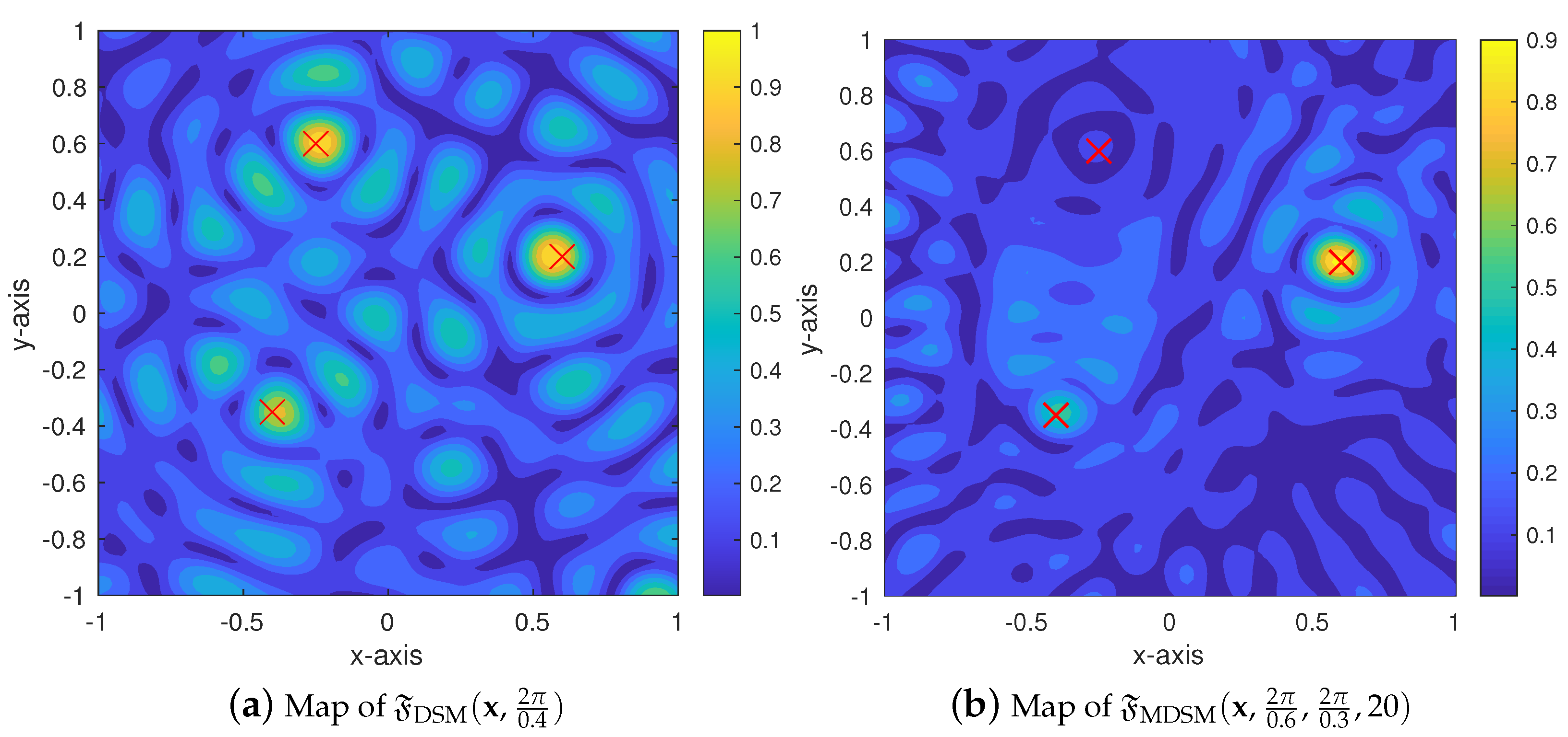
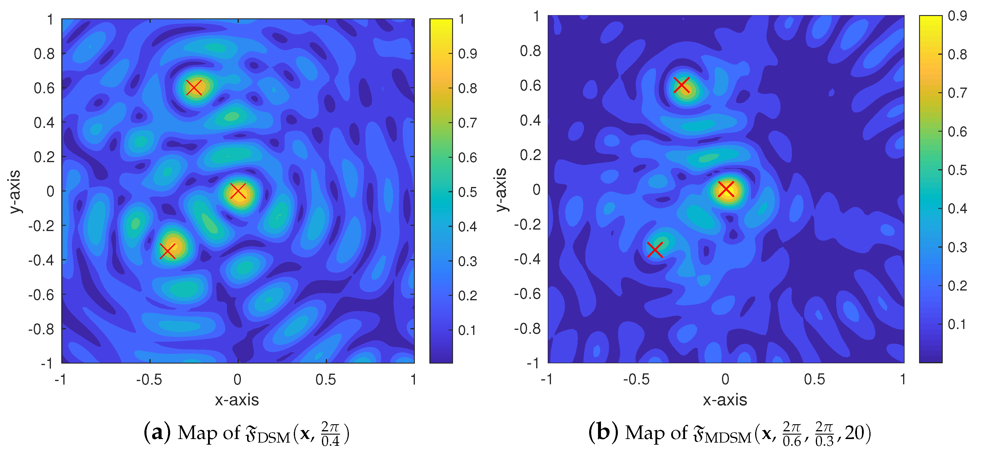
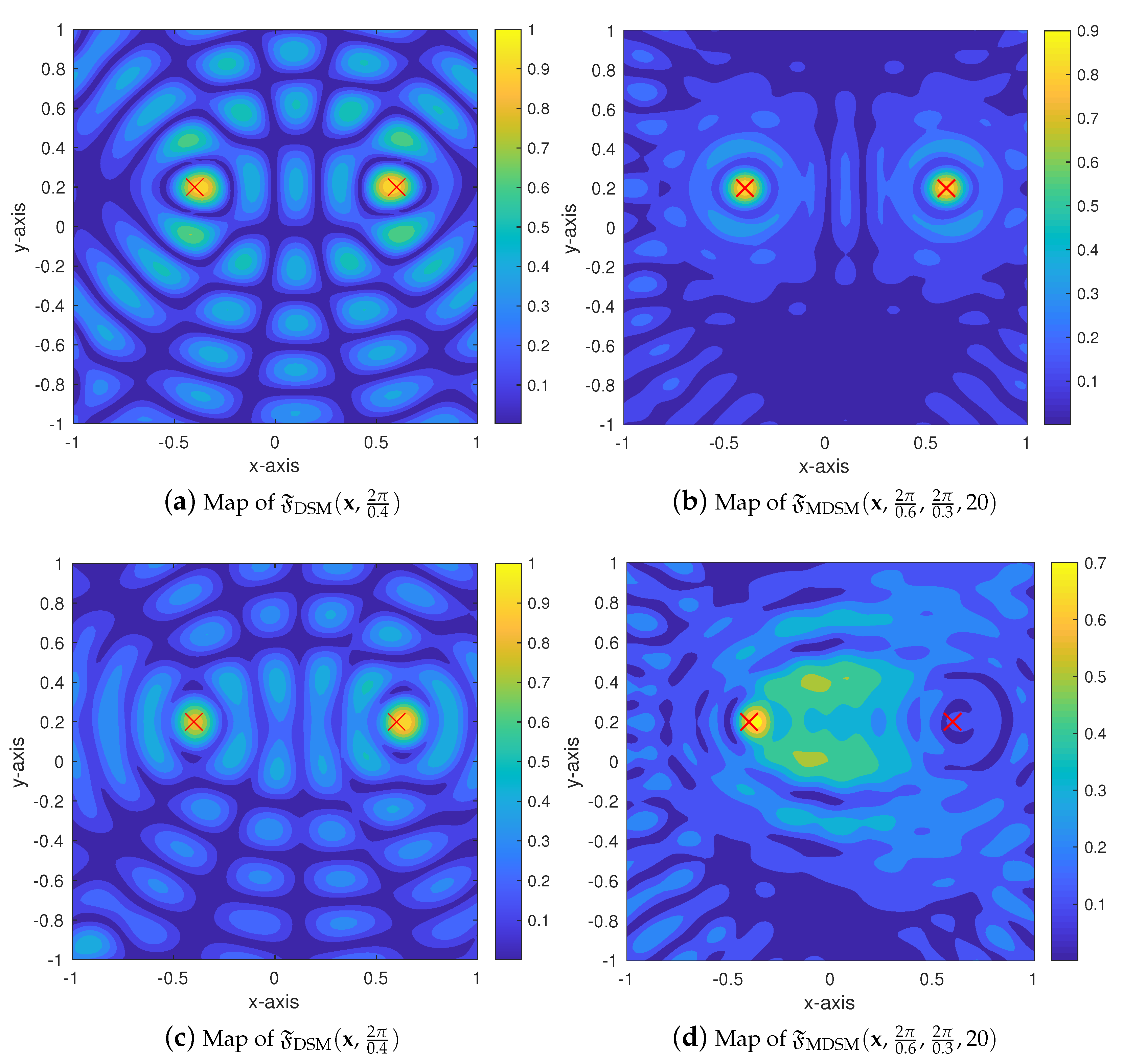
3. Theoretical Reason behind the Non-Improvement of the Multi-Frequency Imaging

In this section, we establish the mathematical theory for explaining the diminishment of the multi-frequency imaging of DSM. Before starting, we recall the following result derived in [11].

Lemma 2.

Assume that the total number of measurement data N is sufficiently large. Then,

$${\mathfrak{F}}_{DSM}(\mathbf{x},k)\approx \frac{\left|\mathrm{\Phi }\right(\mathbf{x},k\left)\right|}{{\displaystyle \underset{\mathbf{x}\in \Omega }{max}\left|\mathrm{\Phi }(\mathbf{x},k)\right|}},$$

where

$$\mathrm{\Phi }(\mathbf{x},k)=\sum _{m=1}^M{e}^{ik\mathbf{d}·{\mathbf{r}}_m}{J}_0\left(k\right|\mathbf{x}-{\mathbf{r}}_m\left|\right).$$

here, $J_n$ denotes the Bessel function of order n of the first kind.

Now, we introduce the main result as follows:

Theorem 1.

Assume that the total number of measurement data N and applied frequencies F are sufficiently large. Then, ${\mathfrak{F}}_{MDSM}(\mathbf{x},k_1,k_F,F)$ can be represented as follows:

$${\mathfrak{F}}_{MDSM}(\mathbf{x},k_1,k_F,F)\approx \frac{\left|\mathrm{\Psi }\right(\mathbf{x}\left)\right|}{{\displaystyle \underset{\mathbf{x}\in \Omega }{max}\left|\mathrm{\Psi }\left(\mathbf{x}\right)\right|}},$$

(7)

where

$$\mathrm{\Psi }\left(\mathbf{x}\right)=\sum _{m\in \mathcal{M}}\left(\mathrm{\Theta }(\mathbf{x},{\mathbf{r}}_m,k_F)-\mathrm{\Theta }(\mathbf{x},{\mathbf{r}}_m,k_1)\right)+\sum _{m\in {\mathcal{M}}^{★}}\left({\mathrm{\Lambda }}_1(\mathbf{x},{\mathbf{r}}_m)+{\mathrm{\Lambda }}_2(\mathbf{x},{\mathbf{r}}_m)\right)$$

(8)

here, $\mathcal{M}=\left\{m:\mathbf{d}·{\mathbf{r}}_m=0\right\}$ and ${\mathcal{M}}^{★}=\left\{m:\mathbf{d}·{\mathbf{r}}_m\ne 0\right\}$. Let $S_n$ denotes the Struve function of order n; then,

$$\begin{array}{c}\mathrm{\Theta }(\mathbf{x},{\mathbf{r}}_m,k)=k{J}_0\left(k\right|\mathbf{x}-{\mathbf{r}}_m\left|\right)\hfill \\ \hfill +\frac{k\pi }{2}\left(J_1\left(k\right|\mathbf{x}-{\mathbf{r}}_m\left|\right)S_0\left(k\right|\mathbf{x}-{\mathbf{r}}_m\left|\right)-J_0\left(k\right|\mathbf{x}-{\mathbf{r}}_m\left|\right)S_1\left(k\right|\mathbf{x}-{\mathbf{r}}_m\left|\right)\right)\end{array}$$

(9)

and

$$\begin{array}{c}\hfill \begin{array}{cc}\hfill {\mathrm{\Lambda }}_1(\mathbf{x},{\mathbf{r}}_m)& =\frac{1}{i\left(\mathbf{d}·{\mathbf{r}}_m\right)}\left(e^{i{k}_F\mathbf{d}·{\mathbf{r}}_m}{J}_0(k_F|\mathbf{x}-{\mathbf{r}}_m\left|\right)-e^{i{k}_1\mathbf{d}·{\mathbf{r}}_m}{J}_0(k_1|\mathbf{x}-{\mathbf{r}}_m\left|\right)\right),\hfill \\ \hfill {\mathrm{\Lambda }}_2(\mathbf{x},{\mathbf{r}}_m)& =\frac{|\mathbf{x}-{\mathbf{r}}_m|}{i\left(\mathbf{d}·{\mathbf{r}}_m\right)}{\int }_{k_1}^{k_F}{e}^{ik\mathbf{d}·{\mathbf{r}}_m}{J}_1\left(k\right|\mathbf{x}-{\mathbf{r}}_m\left|\right)dk.\hfill \end{array}\end{array}$$

(10)

Proof. 

Based on the Lemma 2, we can split

$$\begin{array}{cc}\hfill \frac{\langle u_{\infty }({\theta }_n,\mathbf{d}),e^{-i{k}_f\mathbf{d}·\mathbf{x}}\rangle }{\parallel u_{\infty }({\theta }_n,\mathbf{d}){\parallel }_{L^2\left({\mathbb{S}}^1\right)}{\parallel e^{-i{k}_f\mathbf{d}·\mathbf{x}}\parallel }_{L^2\left({\mathbb{S}}^1\right)}}& =\sum _{m=1}^M{e}^{ik\mathbf{d}·{\mathbf{r}}_m}{J}_0\left(k\right|\mathbf{x}-{\mathbf{r}}_m\left|\right)\hfill \\ \hfill & =\sum _{m\in \mathcal{M}}{J}_0\left(k\right|\mathbf{x}-{\mathbf{r}}_m\left|\right)+\sum _{m\in {\mathcal{M}}^{★}}{e}^{ik\mathbf{d}·{\mathbf{r}}_m}{J}_0\left(k\right|\mathbf{x}-{\mathbf{r}}_m\left|\right).\hfill \end{array}$$

Thus,

$$\begin{array}{c}\sum _{f=1}^F\frac{\langle u_{\infty }({\theta }_n,\mathbf{d}),e^{-i{k}_f\mathbf{d}·\mathbf{x}}\rangle }{\parallel u_{\infty }({\theta }_n,\mathbf{d}){\parallel }_{L^2\left({\mathbb{S}}^1\right)}{\parallel e^{-i{k}_f\mathbf{d}·\mathbf{x}}\parallel }_{L^2\left({\mathbb{S}}^1\right)}}\hfill \\ \hfill \approx {\int }_{k_1}^{k_F}\left(\sum _{m\in \mathcal{M}}{J}_0\left(k\right|\mathbf{x}-{\mathbf{r}}_m\left|\right)+\sum _{m\in {\mathcal{M}}^{★}}{e}^{ik\mathbf{d}·{\mathbf{r}}_m}{J}_0\left(k\right|\mathbf{x}-{\mathbf{r}}_m\left|\right)\right)dk.\end{array}$$

Since the following relation holds (see ([33], Formula 11.1.7)),

$${\int }_0^x{J}_0\left(t\right)dt=x{J}_0\left(x\right)+\frac{x\pi }{2}\left(J_1\left(x\right)S_0\left(x\right)-J_0\left(x\right)S_1\left(x\right)\right),$$

we can obtain

$${\int }_{k_1}^{k_F}\sum _{m\in \mathcal{M}}{J}_0\left(k\right|\mathbf{x}-{\mathbf{r}}_m\left|\right)dk=\sum _{m\in \mathcal{M}}\left(\mathrm{\Theta }(\mathbf{x},{\mathbf{r}}_m,k_F)-\mathrm{\Theta }(\mathbf{x},{\mathbf{r}}_m,k_1)\right),$$

(11)

where the term $\mathrm{\Theta }(\mathbf{x},{\mathbf{r}}_m,k)$ is given in (9).

Since $\frac{d}{dx}{J}_0\left(x\right)=-J_1\left(x\right)$, by performing an integration by parts, we have

$${\int }_{k_1}^{k_F}\sum _{m\in {\mathcal{M}}^{★}}{e}^{ik\mathbf{d}·{\mathbf{r}}_m}{J}_0\left(k\right|\mathbf{x}-{\mathbf{r}}_m\left|\right)dk=\sum _{m\in {\mathcal{M}}^{★}}\left({\mathrm{\Lambda }}_1(\mathbf{x},{\mathbf{r}}_m)+{\mathrm{\Lambda }}_2(\mathbf{x},{\mathbf{r}}_m)\right),$$

(12)

where the terms ${\mathrm{\Lambda }}_1(\mathbf{x},{\mathbf{r}}_m)$ and ${\mathrm{\Lambda }}_2(\mathbf{x},{\mathbf{r}}_m)$ are given in (10). By combining (11) and (12), we can obtain the structure (7). □

Remark 2

(Limitation of multi-frequency DSM). Assume that $\mathbf{d}·{\mathbf{r}}_m\ne 0$ for all $m=1,2,\cdots ,M$. Then, since $J_0\left(0\right)=1$, $J_1\left(x\right)\approx x/2$ when $x\to 0$, and $\mathcal{M}=⌀$ from (8),

$$\mathrm{\Psi }\left(\mathbf{x}\right)=\sum _{m=1}^M\left({\mathrm{\Lambda }}_1(\mathbf{x},{\mathbf{r}}_m)+{\mathrm{\Lambda }}_2(\mathbf{x},{\mathbf{r}}_m)\right).$$

Thus, we can examine that

$$\begin{array}{cc}\hfill \underset{\mathbf{x}\to {\mathbf{r}}_m}{lim}{\mathrm{\Lambda }}_2(\mathbf{x},{\mathbf{r}}_m)& =\underset{\mathbf{x}\to {\mathbf{r}}_m}{lim}\frac{|\mathbf{x}-{\mathbf{r}}_m|}{i\left(\mathbf{d}·{\mathbf{r}}_m\right)}{\int }_{k_1}^{k_F}{e}^{ik\mathbf{d}·{\mathbf{r}}_m}{J}_1\left(k\right|\mathbf{x}-{\mathbf{r}}_m\left|\right)dk.\hfill \\ \hfill & \approx \underset{\mathbf{x}\to {\mathbf{r}}_m}{lim}\frac{|\mathbf{x}-{\mathbf{r}}_m{|}^2}{2i\left(\mathbf{d}·{\mathbf{r}}_m\right)}{\int }_{k_1}^{k_F}k{e}^{ik\mathbf{d}·{\mathbf{r}}_m}dk=0\hfill \end{array}$$

and hence

$$\underset{\mathbf{x}\to {\mathbf{r}}_m}{lim}\mathrm{\Psi }\left(\mathbf{x}\right)\approx \frac{1}{i\left(\mathbf{d}·{\mathbf{r}}_m\right)}\left(e^{i{k}_F\mathbf{d}·{\mathbf{r}}_m}-e^{i{k}_1\mathbf{d}·{\mathbf{r}}_m}\right)implies{\mathfrak{F}}_{MDSM}({\mathbf{r}}_m,F)\propto \frac{1}{|\mathbf{d}·{\mathbf{r}}_m|}.$$

Therefore, ${\mathfrak{F}}_{MDSM}(\mathbf{x},k_1,k_F,F)$ will reach its maximum value at $\mathbf{x}={\mathbf{r}}_{m^{\prime }}$ if $|\mathbf{d}·{\mathbf{r}}_{m^{\prime }}|<|\mathbf{d}·{\mathbf{r}}_m|$ for $m=1,2,\cdots ,M$, $m\ne m^{\prime }$. That means only the location of ${\mathbf{r}}_{m^{\prime }}$ will be identified clearly through the map of ${\mathfrak{F}}_{MDSM}(\mathbf{x},k_1,k_F,F)$ since ${\mathfrak{F}}_{MDSM}({\mathbf{r}}_{m^{\prime }},F)>{\mathfrak{F}}_{MDSM}({\mathbf{r}}_m,F)$, $m=1,2,\cdots ,M$, and $m\ne m^{\prime }$. We refer to Figure 1 and Figure 2 for a detailed description. This is the theoretical reason why only a certain location ${\mathbf{r}}_{m^{\prime }}$ is detected in the multi-frequency DSM in contrast with the single-frequency DSM. Moreover, if there exists a single inhomogeneity, its location can be identified through the map of ${\mathfrak{F}}_{MDSM}(\mathbf{x},k_1,k_F,F)$ for any $\mathbf{d}$.

Remark 3

(Identifiable locations). Notice that if two locations ${\mathbf{r}}_{m^{\prime }}$ and ${\mathbf{r}}_{m^{″}}$ satisfy $|\mathbf{d}·{\mathbf{r}}_{m^{\prime }}|\approx |\mathbf{d}·{\mathbf{r}}_{m^{″}}|$, their locations can be identified simultaneously via the map of ${\mathfrak{F}}_{MDSM}(\mathbf{x},k_1,k_F,F)$; refer to Figure 2a. Moreover, if a crack ${\mathrm{\Gamma }}_{m^{\prime }}$ is located at the origin ($\mathbf{d}·{\mathbf{r}}_{m^{\prime }}=0$ for any $\mathbf{d}$), then since $J_0\left(0\right)=1$, $J_1\left(0\right)=0$, $S_1\left(0\right)=0$, and $S_2\left(0\right)=0$,

$$\underset{\mathbf{x}\to {\mathbf{r}}_{m^{\prime }}}{lim}\left(\mathrm{\Theta }(\mathbf{x},{\mathbf{r}}_m,k_F)-\mathrm{\Theta }(\mathbf{x},{\mathbf{r}}_m,k_1)\right)=k_F-k_1.$$

This means that ${\mathfrak{F}}_{MDSM}({\mathbf{r}}_{m^{\prime }},F)\approx 1$ for $m\ne m^{\prime }$; thus, the location ${\mathbf{r}}_{m^{\prime }}$ can always be identified through the map of ${\mathfrak{F}}_{MDSM}(\mathbf{x},k_1,k_F,F)$ for any $\mathbf{d}$, as shown in Figure 2b.

Remark 4.

In order to identify the location ${\mathbf{r}}_m$ through the map of ${\mathfrak{F}}_{MDSM}(\mathbf{x},k_1,k_F,F)$, one must select an incident direction that satisfies $\mathbf{d}·{\mathbf{r}}_m=0$. However, the identification of every location of cracks with a single incident direction will be difficult, since we have no a priori information of ${\mathbf{r}}_m$. This is the theoretical reason why multiple incident fields must be applied to obtain good results; refer to [1,11,27].

Remark 5.

According to [17], the indicator function of the orthogonality sampling method (OSM) is equivalent to the that for DSM. Therefore, it can be said that based on the aforementioned descriptions in Remarks 2–4, multi-frequency indicator function of OSM (6) did not yield a reasonable reconstruction examined by the numerical simulation results of ([27], Section 3.3).

4. Simulation Results and Discussion

In this section, we exhibit numerical simulation results to support the theoretical result. For this, we applied $k=\frac{2\pi }{0.4}$ for single-frequency imaging and $F=20$ different wavenumbers with $k_1=\frac{2\pi }{0.6}$ and $k_F=\frac{2\pi }{0.3}$ for multi-frequency imaging. The imaging region $\Omega$ was set to $\Omega =[-1,1]\times [-1,1]$, and the values of ${\mathfrak{F}}_{DSM}(\mathbf{x},\frac{2\pi }{0.4})$ and ${\mathfrak{F}}_{MDSM}(\mathbf{x},\frac{2\pi }{0.6},\frac{2\pi }{0.3},20)$ were evaluated for each $\mathbf{x}\in \Omega$. The far-field pattern data $u_{\infty }({\theta }_n,\mathbf{d})$, $n=1,2,\cdots ,N=30$, was generated by solving a Fredholm integral equation of the second kind along the cracks; refer to ([34], Chapter 4). After the generation of the far-field pattern data, a $20$ dB white Gaussian random noise was added. Throughout this section, the length of all cracks is chosen as $\ell =0.05$.

Example 1.

Figure 3 shows maps of ${\mathfrak{F}}_{DSM}(\mathbf{x},\frac{2\pi }{0.4})$ and ${\mathfrak{F}}_{MDSM}(\mathbf{x},\frac{2\pi }{0.6},\frac{2\pi }{0.3},20)$ for $\mathbf{d}=(1,0)$ in the presence of three small cracks located at ${\mathbf{r}}_1=(0.60,0.20)$, ${\mathbf{r}}_2=(-0.20,-0.60)$, and ${\mathbf{r}}_3=(-0.40,-0.35)$. Notice that peaks of large magnitude appeared at the location of all cracks ${\mathrm{\Gamma }}_m$ in the map of ${\mathfrak{F}}_{DSM}(\mathbf{x},\frac{2\pi }{0.4})$, so it is possible to identify the location of cracks. However, since $|\mathbf{d}·{\mathbf{r}}_1|=0.60$, $|\mathbf{d}·{\mathbf{r}}_2|=0.20$, and $|\mathbf{d}·{\mathbf{r}}_3|=0.40$, only the location ${\mathbf{r}}_2$ can be identified through the map of ${\mathfrak{F}}_{MDSM}(\mathbf{x},\frac{2\pi }{0.6},\frac{2\pi }{0.3},20)$.

Example 2.

Figure 4 shows maps of ${\mathfrak{F}}_{DSM}(\mathbf{x},\frac{2\pi }{0.4})$ and ${\mathfrak{F}}_{MDSM}(\mathbf{x},\frac{2\pi }{0.6},\frac{2\pi }{0.3},20)$ with the same simulation configuration of Example 1 except the lengths of the cracks are equal to $2\ell =0.1$. By regarding the result, we can observe similar phenomenon so if the length of the cracks is the same, the identification via multi-frequency DSM is dependent on the propagation direction and independent of the crack length.

Example 3.

Figure 5 shows maps of ${\mathfrak{F}}_{MDSM}(\mathbf{x},k_1,k_F,20)$ for various $k_1$ and $k_F$ with the same simulation configuration of Example 1. It is interesting to examine that opposite to the simulation result in Example 1, the location of ${\mathbf{r}}_3$ can be identified clearly when $k_1=\frac{2\pi }{0.8}$ and $k_F=\frac{2\pi }{0.5}$. Notice that a peak of small magnitude appeared at the location ${\mathbf{r}}_1$ when $k_1=\frac{2\pi }{0.8}$ and $k_F=\frac{2\pi }{0.5}$; however, due to the appearance of several artifacts in the map, it will be hard to conclude the existence of any cracks. Throughout the map of ${\mathfrak{F}}_{MDSM}(\mathbf{x},\frac{2\pi }{0.4},\frac{2\pi }{0.2},20)$, it is very hard to identify all cracks due to the appearance of artifacts with large magnitude. Therefore, a theoretical exploration of the selection of the range of wavenumbers will be a notable subject.

Example 4.

Figure 6 shows maps of ${\mathfrak{F}}_{DSM}(\mathbf{x},\frac{2\pi }{0.4})$ and ${\mathfrak{F}}_{MDSM}(\mathbf{x},\frac{2\pi }{0.6},\frac{2\pi }{0.3},20)$ with the same configuration as in Example 1, except that the propagation direction $\mathbf{d}=(0,1)$. Similar to Example 1, it is possible to identify the location of cracks through the map of ${\mathfrak{F}}_{DSM}(\mathbf{x},\frac{2\pi }{0.4})$. In contrast, only the location ${\mathbf{r}}_1$ can be identified through the map of ${\mathfrak{F}}_{MDSM}(\mathbf{x},\frac{2\pi }{0.6},\frac{2\pi }{0.3},20)$ because $|\mathbf{d}·{\mathbf{r}}_1|=0.20<|\mathbf{d}·{\mathbf{r}}_2|=0.60$ and $|\mathbf{d}·{\mathbf{r}}_3|=0.35$.

Example 5.

Figure 7 shows maps of ${\mathfrak{F}}_{DSM}(\mathbf{x},\frac{2\pi }{0.4})$ and ${\mathfrak{F}}_{MDSM}(\mathbf{x},\frac{2\pi }{0.6},\frac{2\pi }{0.3},20)$ with the same configuration as in Example 1, except that the location ${\mathbf{r}}_1=(0,0)$. Since $|\mathbf{d}·{\mathbf{r}}_1|=0$, the location of ${\mathbf{r}}_1$ can be identified through the map of ${\mathfrak{F}}_{MDSM}(\mathbf{x},\frac{2\pi }{0.6},\frac{2\pi }{0.3},20)$. Moreover, since $|\mathbf{d}·{\mathbf{r}}_2|=0.20<|\mathbf{d}·{\mathbf{r}}_3|=0.40$, the location of ${\mathbf{r}}_2$ can also be recognized.

Example 6.

Figure 8 shows maps of ${\mathfrak{F}}_{DSM}(\mathbf{x},\frac{2\pi }{0.4})$ and ${\mathfrak{F}}_{MDSM}(\mathbf{x},\frac{2\pi }{0.6},\frac{2\pi }{0.3},20)$ with the same configuration as in Example 5, except that the propagation direction is now $\mathbf{d}=(0,1)$. Similarly with Example 5, the location of ${\mathbf{r}}_1$ can be identified through the map of ${\mathfrak{F}}_{MDSM}(\mathbf{x},\frac{2\pi }{0.6},\frac{2\pi }{0.3},20)$ because $|\mathbf{d}·{\mathbf{r}}_1|=0$. In contrast to Example 5, although $|\mathbf{d}·{\mathbf{r}}_2|=0.60>|\mathbf{d}·{\mathbf{r}}_3|=0.35$, it is difficult to recognize the location of ${\mathbf{r}}_3$ due to the appearance of several artifacts in the neighborhood of ${\mathbf{r}}_3$. Notice that although several artifacts are included, three location of cracks can be identified through the map of ${\mathfrak{F}}_{DSM}(\mathbf{x},\frac{2\pi }{0.4})$ for any selection of $\mathbf{d}$.

Example 7.

Figure 9 shows maps of ${\mathfrak{F}}_{DSM}(\mathbf{x},\frac{2\pi }{0.4})$ and ${\mathfrak{F}}_{MDSM}(\mathbf{x},\frac{2\pi }{0.6},\frac{2\pi }{0.3},20)$ for $\mathbf{d}=(0,1)$ in the presence of three small cracks located at ${\mathbf{r}}_1=(0,0)$, ${\mathbf{r}}_2=(-0.20,-0.60)$, and ${\mathbf{r}}_3=(0.60,0)$. Since $|\mathbf{d}·{\mathbf{r}}_1|=0$ and $|\mathbf{d}·{\mathbf{r}}_3|=0$, the location of both ${\mathbf{r}}_1$ and ${\mathbf{r}}_3$ can be identified through the map of ${\mathfrak{F}}_{MDSM}(\mathbf{x},\frac{2\pi }{0.6},\frac{2\pi }{0.3},20)$. However, since $|\mathbf{d}·{\mathbf{r}}_2|=0.60\gg |\mathbf{d}·{\mathbf{r}}_1|,|\mathbf{d}·{\mathbf{r}}_3|$, it is very hard to recognize the location of ${\mathbf{r}}_2$. Similarly with Example 6, since $|\mathbf{d}·{\mathbf{r}}_1|=0$ and $|\mathbf{d}·{\mathbf{r}}_2|=0.20<|\mathbf{d}·{\mathbf{r}}_3|=0.60$, both ${\mathbf{r}}_1$ and ${\mathbf{r}}_2$ can be identified through the map of ${\mathfrak{F}}_{MDSM}(\mathbf{x},\frac{2\pi }{0.6},\frac{2\pi }{0.3},20)$ with $\mathbf{d}=(1,0)$; refer to the bottom line of Figure 9.

Example 8.

Figure 10 shows maps of ${\mathfrak{F}}_{DSM}(\mathbf{x},\frac{2\pi }{0.4})$ and ${\mathfrak{F}}_{MDSM}(\mathbf{x},\frac{2\pi }{0.6},\frac{2\pi }{0.3},20)$ for $\mathbf{d}=(0,1)$ in the presence of two small cracks located at ${\mathbf{r}}_1=(0.60,0.20)$ and ${\mathbf{r}}_2=(-0.40,0.20)$. Notice that since $|\mathbf{d}·{\mathbf{r}}_1|=|\mathbf{d}·{\mathbf{r}}_2|=0$, although the x-axis positions are different, the location of two cracks can be identified through the map of ${\mathfrak{F}}_{MDSM}(\mathbf{x},\frac{2\pi }{0.6},\frac{2\pi }{0.3},20)$. However, if one selects the propagation direction $\mathbf{d}=(1,0)$, it is very hard to identify ${\mathbf{r}}_1$ through the map of ${\mathfrak{F}}_{MDSM}(\mathbf{x},\frac{2\pi }{0.6},\frac{2\pi }{0.3},20)$, but it is possible through the map of ${\mathfrak{F}}_{DSM}(\mathbf{x},\frac{2\pi }{0.4})$; refer to the bottom line of Figure 10.

5. Conclusions

In this study, we considered multi-frequency DSM for a fast recognition of linear perfectly conducting cracks with small length from measured far-field pattern data. To account for the non-improvement of the multi-frequency DSM against the single-frequency one, the mathematical structure of indicator function of multi-frequency DSM were analyzed by establishing a relationship between Bessel and Struve functions and the incident plane-wave.

In this paper, we considered the crack with Dirichlet boundary condition. Application and analysis to the crack with Neumann boundary condition will be the forthcoming work. In the limited-aperture inverse scattering problem, similar phenomena can be examined. Extension to the limited-aperture problem will be the subject of a forthcoming work. Finally, extending the application and analysis to the 3D inverse scattering problem or real-world microwave imaging will be an interesting and remarkable research subject.

References

1. Ito, K.; Jin, B.; Zou, J. A direct sampling method to an inverse medium scattering problem. Inverse Prob. 2012, 28, 025003. [Google Scholar] [CrossRef]
2. Ito, K.; Jin, B.; Zou, J. A direct sampling method for inverse electromagnetic medium scattering. Inverse Prob. 2013, 29, 095018. [Google Scholar] [CrossRef] [Green Version]
3. Li, J.; Zou, J. A direct sampling method for inverse scattering using far-field data. Inverse Probl. Imag. 2013, 7, 757–775. [Google Scholar] [CrossRef]
4. Kang, S.; Lambert, M.; Park, W.K. Direct sampling method for imaging small dielectric inhomogeneities: Analysis and improvement. Inverse Prob. 2018, 34, 095005. [Google Scholar] [CrossRef] [Green Version]
5. Kang, S.; Lambert, M. Structure analysis of direct sampling method in 3D electromagnetic inverse problem: Near- and far-field configuration. Inverse Prob. 2021, 37, 075002. [Google Scholar] [CrossRef]
6. Chow, Y.T.; Ito, K.; Zou, J. A direct sampling method for electrical impedance tomography. Inverse Prob. 2014, 30, 095003. [Google Scholar] [CrossRef] [Green Version]
7. Chow, Y.T.; Ito, K.; Liu, K.; Zou, J. Direct sampling method for diffusive optical tomography. SIAM J. Sci. Comput. 2015, 37, A1658–A1684. [Google Scholar] [CrossRef]
8. Kang, S.; Lambert, M.; Park, W.K. Analysis and improvement of direct sampling method in the mono-static configuration. IEEE Geosci. Remote Sens. Lett. 2019, 16, 1721–1725. [Google Scholar] [CrossRef]
9. Liu, K.; Xu, Y.; Zou, J. A multilevel sampling method for detecting sources in a stratified ocean waveguide. J. Comput. Appl. Math. 2017, 309, 95–110. [Google Scholar] [CrossRef] [Green Version]
10. Liu, K. A simple method for detecting scatterers in a stratified ocean waveguide. Comput. Math. Appl. 2018, 76, 1791–1802. [Google Scholar] [CrossRef]
11. Park, W.K. Direct sampling method for retrieving small perfectly conducting cracks. J. Comput. Phys. 2018, 373, 648–661. [Google Scholar] [CrossRef] [Green Version]
12. Ahn, C.Y.; Ha, T.; Park, W.K. Direct sampling method for identifying magnetic inhomogeneities in limited-aperture inverse scattering problem. Comput. Math. Appl. 2020, 80, 2811–2829. [Google Scholar] [CrossRef]
13. Park, W.K. Direct sampling method for anomaly imaging from scattering parameter. Appl. Math. Lett. 2018, 81, 63–71. [Google Scholar] [CrossRef] [Green Version]
14. Ji, X.; Liu, X.; Zhang, B. Phaseless inverse source scattering problem: Phase retrieval, uniqueness and direct sampling methods. J. Comput. Phys. X 2019, 1, 100003. [Google Scholar] [CrossRef]
15. Son, S.H.; Lee, K.J.; Park, W.K. Application and analysis of direct sampling method in real-world microwave imaging. Appl. Math. Lett. 2019, 96, 47–53. [Google Scholar] [CrossRef] [Green Version]
16. Liu, K. Two effective post-filtering strategies for improving direct sampling methods. Appl. Anal. 2017, 96, 502–515. [Google Scholar] [CrossRef]
17. Harris, I.; Nguyen, D.L. Orthogonality sampling method for the electromagnetic inverse scattering problem. SIAM J. Sci. Comput. 2020, 42, B722–B737. [Google Scholar] [CrossRef]
18. Ammari, H.; Garnier, J.; Kang, H.; Park, W.K.; Sølna, K. Imaging schemes for perfectly conducting cracks. SIAM J. Appl. Math. 2011, 71, 68–91. [Google Scholar] [CrossRef] [Green Version]
19. Park, W.K. Multi-frequency subspace migration for imaging of perfectly conducting, arc-like cracks in full- and limited-view inverse scattering problems. J. Comput. Phys. 2015, 283, 52–80. [Google Scholar] [CrossRef] [Green Version]
20. Alqadah, H.F.; Valdivia, N. A frequency based constraint for a multi-frequency linear sampling method. Inverse Prob. 2013, 29, 095019. [Google Scholar] [CrossRef]
21. Guzina, B.; Cakoni, F.; Bellis, C. On the multi-frequency obstacle reconstruction via the linear sampling method. Inverse Prob. 2010, 26, 125005. [Google Scholar] [CrossRef] [Green Version]
22. Funes, J.F.; Perales, J.M.; Rapún, M.L.; Vega, J.M. Defect detection from multi-frequency limited data via topological sensitivity. J. Math. Imaging Vis. 2016, 55, 19–35. [Google Scholar] [CrossRef]
23. Park, W.K. Performance analysis of multi-frequency topological derivative for reconstructing perfectly conducting cracks. J. Comput. Phys. 2017, 335, 865–884. [Google Scholar] [CrossRef] [Green Version]
24. Moscoso, M.; Novikov, A.; Papanicolaou, G.; Tsogka, C. Robust multifrequency imaging with MUSIC. Inverse Prob. 2018, 35, 015007. [Google Scholar] [CrossRef] [Green Version]
25. Solimene, R.; Ruvio, G.; Dell’Aversano, A.; Cuccaro, A.; Ammann, M.J.; Pierri, R. Detecting point-like sources of unknown frequency spectra. Prog. Electromagn. Res. B 2013, 50, 347–364. [Google Scholar] [CrossRef] [Green Version]
26. Park, W.K. Negative result of multi-frequency direct sampling method in microwave imaging. Results Phys. 2019, 12, 859–860. [Google Scholar] [CrossRef]
27. Potthast, R. A study on orthogonality sampling. Inverse Prob. 2010, 26, 074015. [Google Scholar] [CrossRef]
28. Alzaalig, A.; Hu, G.; Liu, X.; Sun, J. Fast acoustic source imaging using multi-frequency sparse data. Inverse Prob. 2020, 36, 025009. [Google Scholar] [CrossRef] [Green Version]
29. Arens, T.; Ji, X.; Liu, X. Inverse electromagnetic obstacle scattering problems with multi-frequency sparse backscattering far field data. Inverse Prob. 2020, 36, 105007. [Google Scholar] [CrossRef]
30. Kang, S.; Lambert, M.; Ahn, C.Y.; Ha, T.; Park, W.K. Single- and multi-frequency direct sampling methods in limited-aperture inverse scattering problem. IEEE Access 2020, 8, 121637–121649. [Google Scholar] [CrossRef]
31. Kress, R. Inverse scattering from an open arc. Math. Meth. Appl. Sci. 1995, 18, 267–293. [Google Scholar] [CrossRef]
32. Ammari, H.; Kang, H.; Lee, H.; Park, W.K. Asymptotic imaging of perfectly conducting cracks. SIAM J. Sci. Comput. 2010, 32, 894–922. [Google Scholar] [CrossRef]
33. Abramowitz, M.; Stegun, I.A. Handbook of Mathematical Functions, with Formulas, Graphs, and Mathematical Tables; Dover: New York, NY, USA, 1996. [Google Scholar]
34. Nazarchuk, Z.T. Singular Integral Equations in Diffraction Theory; Mathematics and Applications Series; Karpenko Physicomechanical Institute, Ukrainian Academy of Sciences: Lviv, Ukraine, 1994.
Figure 1. (Remark 2) Illustration of identifiable locations through the map of F MDSM ( x , k 1 , k F , F ) .
Mathematics 10 01674 g001
Figure 2. (Remark 3) Illustration of identifiable locations through the map of F MDSM ( x , k 1 , k F , F ) .
Mathematics 10 01674 g002
Figure 3. (Example 1) Simulation results with d = ( 1 , 0 ) . The red-colored marks × denote the locations of cracks.
Mathematics 10 01674 g003
Figure 4. (Example 2) Simulation results with d = ( 1 , 0 ) . The red-colored marks × denote the locations of cracks.
Mathematics 10 01674 g004
Figure 5. (Example 3) Simulation results with d = ( 1 , 0 ) . The red-colored marks × denote the locations of cracks.
Mathematics 10 01674 g005
Figure 6. (Example 4) Simulation results with d = ( 0 , 1 ) . The red-colored marks × denote the locations of cracks.
Mathematics 10 01674 g006
Figure 7. (Example 5) Simulation results with d = ( 1 , 0 ) . The red-colored marks × denote the locations of cracks.
Mathematics 10 01674 g007
Figure 8. (Example 6) Simulation results with d = ( 0 , 1 ) . The red-colored marks × denote the locations of cracks.
Mathematics 10 01674 g008
Figure 9. (Example 7) Simulation results with d = ( 0 , 1 ) (top line) and d = ( 1 , 0 ) (bottom line). The red-colored marks × denote the location of cracks.
Mathematics 10 01674 g009
Figure 10. (Example 8) Simulation results with d = ( 1 , 0 ) . The red-colored marks × denote the locations of cracks.
Mathematics 10 01674 g010
Publisher’s Note: MDPI stays neutral with regard to jurisdictional claims in published maps and institutional affiliations.