Capacity-Oriented Train Scheduling of High-Speed Railway Considering the Operation and Maintenance of Rolling Stock

Abstract

The capacity of some busy rail lines is increasingly tight and passenger demand far exceeds the railway capacity. To schedule as many trains as possible in order to satisfy more transportation demands, we studied the capacity-oriented train scheduling problem. While most approaches focus only on increasing the capacity of the rail line, this research considers both the time-space distribution of transportation demands and the operation and maintenance of rolling stock. To solve this problem, we first constructed a time-space network to describe the time-space path of rolling stock. We then proposed an integer planning model with rolling stock maintenance and the OD service frequency constraints to maximize the number of running arcs in rail sections. After decomposing this model by introducing some Lagrangian multipliers to relax its hard constraints, we proposed a Lagrangian relaxation-based decomposition algorithm, including two path search sub-algorithms for rolling stock to optimize both the relaxed and the feasible solutions. Finally, we conducted a computation study on a practical double-track high-speed railway line to test the performance of this algorithm. It reports that the train timetables and the operation of rolling stock are well managed.

1. Introduction

A train timetable is the basis of transportation organization. It specifies the departure and arrival times of trains at each visited station. It is highly valued by railway companies as it ensures the safe operation of trains and effective coordination among all related departments in the rail system. Moreover, since it affects the transportation efficiency and the quality of passenger travel service, it determines whether the passengers decide to travel by train. Optimizing train scheduling will not only help to reduce the operating costs of the railway company, but it will also help to provide high-quality travel services for passengers. In other words, it is beneficial to attract more passengers and increase the benefits of the railway company. As demand for rail services grows with passenger numbers, fixing the train scheduling problem is critical in the operation and management of a high-speed railway.

Generally speaking, train scheduling problems are divided into cost-oriented problems and demand-oriented problems. Cost-oriented train timetabling aims to improve transportation efficiency and lower operating costs on the basis of passenger satisfaction. The optimization objectives usually include minimizing trains’ total travel time, maximizing the total benefit of the railway company, and reducing trains’ delays at stations, etc. For instance, Shi et al. [1] improved transportation efficiency by minimizing trains’ total travel time and turnaround time. Zhou et al. [2] adopted the sequential optimization method to optimize train timetables to minimize the total trains’ travel time. Cacchiani et al. [3] designed two relaxation-based heuristics and precise algorithms to maximize the operating profit for railway companies. Furthermore, some studies proposed to reduce trains’ delays to optimize train scheduling, such as Xu et al. [4] and Li et al. [5]. Additionally, some studies such as Shafia et al. [6], Su et al. [7], Bešinović et al. [8], and Robenek et al. [9] optimized train scheduling for the purpose of improving robustness and saving energy. However, the demand-oriented train timetabling problem intends to save passengers’ travel time and improve passenger satisfaction. For example, Goerigk and Schöbel [10] designed a periodic timetabling model with the goal of minimizing passengers’ travel time. Wong et al. [11] proposed a timetabling model to minimize the waiting time for transfer passengers. Kroon et al. [12] took reducing the sum of passengers’ waiting time and travel time as the optimization objective. Huang et al. [13] developed a method to optimize uneven running train timetables by considering passenger departure time and seat-class preferences.

With the enormous transportation demand on some busy rail lines, their capacity is increasingly tight. Therefore, the capacity-oriented problem has recently received increasing attention. It aims to make full use of transportation capacity in order to operate more trains. A great deal of research considers transportation organization as a major factor affecting capacity. Chen et al. [14] proposed a timing-cycle iterative method to maximize the number of scheduled trains by considering the combination of the train stop plan and speed level. Boroun et al. [15] proposed a new mathematical programming approach to maximize the railway infrastructure capacity by minimizing the schedule makespan. Lu et al. [16] proposed different train speed level ratios to maximize the utilization of railway capacity. Dong and Siji [17] aimed to minimize the average minimum interval time for increasing the capacity for rail sections. Some works transformed this problem into a multi-commodity network flow problem, such as Harrod [18] and Azadi et al. [19]. Compared with the existing studies for capacity-oriented train scheduling problems, most of them only focus on the train operational factor. Our work differs from these studies in that our model generates train scheduling and rolling stock scheduling simultaneously.

In recent years, many integrated models of train timetable and rolling stock circulation have been proposed. Olsson [20] analyzed how the interaction between train timetables and rolling stock affects train punctuality. Veelenturf et al. [21] studied the integrated optimization for train rescheduling and rolling stock circulation. Liao et al. [22] formulated an integrated model to maximize transportation performance and proposed a Lagrangian relaxation decomposition method. These approaches provide strong support for the integrated capacity-oriented optimization. Similarly, our model generates train scheduling and rolling stock circulation simultaneously. Unfortunately, few studies have focused on the impact of rolling stock maintenance on capacity. Therefore, our model involves the daily rolling stock maintenance problem, which is an important area in railway operations. The related works include the rolling stock maintenance problem typically proposed as a two-step approach that combines the scheduling tasks related to train services, such as Giacco et al. [23] and Zhong et al. [24].

Compared with the existing studies for capacity-oriented train scheduling, they assume a set of trains given in advance and aim to calculate the maximum number of trains that can be feasibly scheduled. Our approach does not pre-determine candidate trains, but rather provides a set of candidate routes and stop plans. Particularly, some service requirements are considered to match trains’ scheduling with the time-space distribution of transportation demand, such as the minimum dwell rate of trains at each station and the minimum number of trains to serve each OD.

This paper studies the capacity-oriented train scheduling problem on a busy high-speed rail line whose transportation demand far exceeds the railway capacity. Our model aims to schedule as many trains as possible into a timetable and enables them to match the time-space distribution of transportation demand. We also consider the operation and maintenance of rolling stock. In this way, we can increase the transportation capacity and ensure the practical operation of the train timetable. This research will provide the following major contributions in the area of train scheduling optimization.

• The capacity-oriented train scheduling not only matches train services with the time-space distribution of transportation demand, but also ensures rolling stock maintenance. In this way, we can provide more train services to meet all OD travel demand and ensure the practical operation of rolling stock scheduling.
• A time-space network is designed to describe the operation of rolling stock. Based on this time-space network, an integer programming model is formulated to maximize the number of running arcs, so that we can increase the operating time of rolling stock in rail sections to provide more train services.
• A Lagrangian relaxation-based decomposition algorithm is designed, and it contains two path search sub-algorithms for optimizing the upper and lower bounds corresponding to the relaxation and feasible solutions, respectively. This algorithm can not only solve our model efficiently, but also optimize the quality of train scheduling.

The rest of this paper is organized as follows. In Section 2, the time-space network is presented and the problem is described in detail. In Section 3, the optimization model is presented. In Section 4, the decomposition model based on Lagrangian relaxation is presented. In Section 5, the design of the Lagrangian relaxation-based decomposition algorithm is described. In Section 6, we discuss the practical case of the Wuhan-Guangzhou high-speed railway to verify the validity of the model and the algorithm. In Section 7, some conclusions and future studies are given.

2. Capacity-Oriented Train Scheduling Problem Description

We study the train scheduling problem by considering the operation and maintenance of rolling stock. While a rolling stock unit can serve multiple trains in its operation hours, we aim to simultaneously determine the trains scheduling and the rolling stock scheduling. Our problem is based on a double-track high-speed rail line composed of rail sections, stations and depots. Trains can stop at any station for passengers to board and alight, but can only turn around at stations with turnaround capability. A depot is an area of tracks close to a station and provides parking or maintenance services for rolling stock. In addition, there are two types of depots, namely parking depots and maintenance depots. All rolling stock units are assumed to be initially and finally placed in depots. Particularly, only stations that are directly connected to depots can be used as origins and destinations of rolling stock.

2.1. Time-Space Network Construction

We design a time-space network composed of multiple types of nodes and arcs to describe the time-space paths of rolling stock units and their serving trains. $S$ represents the set of stations, and $S_z\in S$ represents the set of stations with turnaround capability. $S_y$ represents the set of depots and $y_k\in S_y$ represents a depot connected with a station $k\in S$. In addition, the parking depot is denoted as $\dot{y}\in S_y$, while the maintenance depot is denoted as $\ddot{y}\in S_y$. Given the rail line and planning time horizon, the nodes and arcs of the time-space network can be constructed as follows.

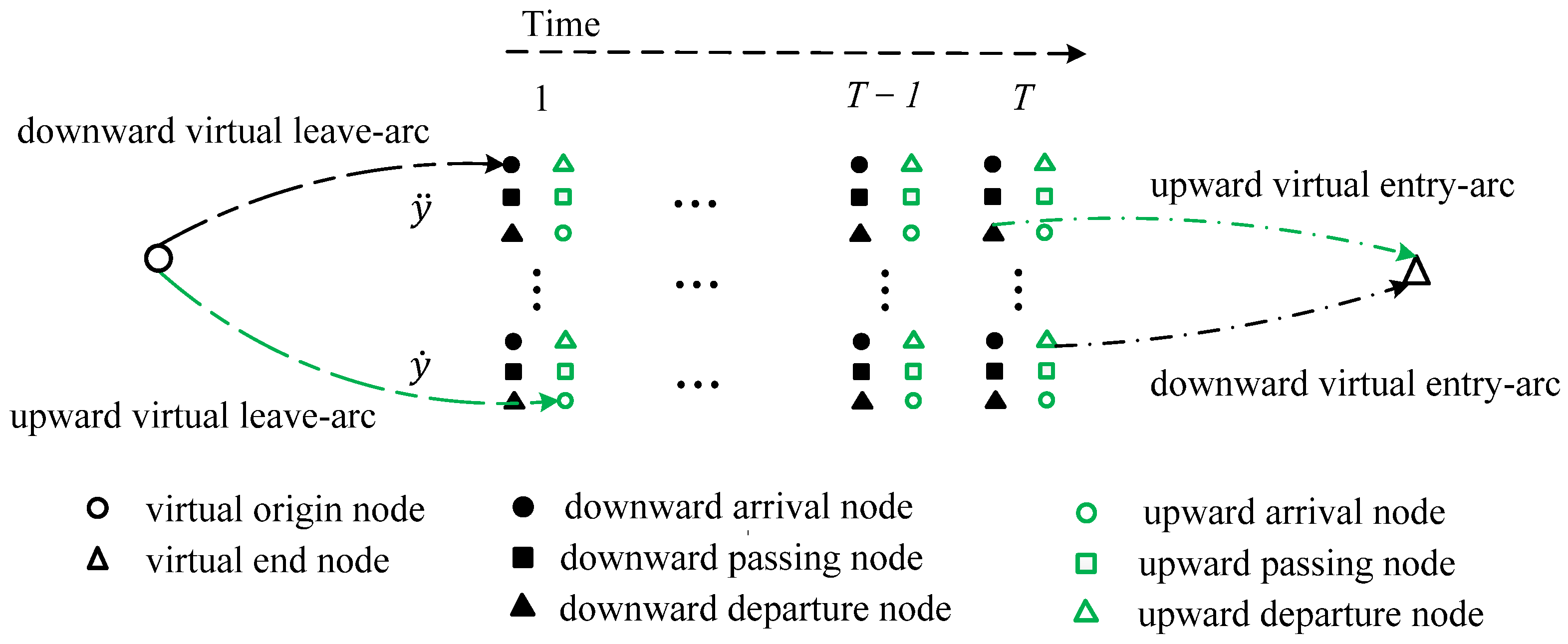
2.1.1. Nodes Construction

Each station is discretized as a set of arrival, departure and passing nodes by incorporating the time dimension. Furthermore, we construct the upward and downward arrival, departure and passing nodes to distinguish the direction. For a station $k$, we denote $u_{k,d}^t$, $w_{k,d}^t$, $v_{k,d}^t$ to represent arrival, passing and departure nodes in the direction $d$ at time $t$, respectively. When $d=1$, it indicates the downward direction, and when $d=0$, it indicates the upward direction. In addition, since the initial position of each rolling stock unit is not pre-specified, we assume a rolling stock unit will depart from a virtual origin node and return to a virtual end node on the time-space network, which are denoted as $\overline{o}$ and $\overline{d}$, respectively.

2.1.2. Directed Arcs Construction

Five types of directed arcs re constructed among the arrival, departure and passing nodes as follows.

• Virtual arcs

In the Chinese high-speed railway, rolling stock units stay in depots and are maintained at night. In other words, rolling stock units must leave depots in the morning and return to depots at night. To indicate the starting place and time of a rolling stock unit, a virtual leave-arc denoted as ${\hat{a}}_k^t=\left(\overline{o},u_{k,d}^t\right)$ is constructed from the virtual node $\overline{o}$ to an arrival node $u_{k,d}^t$ if $y_k\in S_y$ and $t=1,\dots ,T-1$. Similarly, to indicate the ending place and time of a rolling stock unit, a virtual entry-arc denoted as ${\check{a}}_k^t=\left(v_{k,d}^t,\overline{d}\right)$ is constructed from departure node $v_{k,d}^t$ to the virtual end node $\overline{d}$ if $y_k\in S_y$ and $t=1,\dots ,T$. These two kinds of arcs are shown in Figure 1.

2.

Running arcs in rail sections

The running arcs are constructed to describe trains running in rail sections. Let $E$ present the set of rail sections, and each rail section $\left(k,k^{\prime }\right)\in E$ presents the track segment from station $k$ to station $k^{\prime }$, with no intermediate station in between. Based on whether a train stops at stations in a rail section, trains running is divided into four situations: pass-pass, departure-pass, pass-arrival, and departure-arrival. Denoted $t_{k,k^{\prime }}$ as the minimum running time in the rail section $\left(k,k^{\prime }\right)$, and $t_s$, $t_b$ as the additional times for decelerating and accelerating, respectively. In the rail section $\left(k,k^{\prime }\right)$, the four kinds of running arcs are constructed as follows.

• Pass-Pass (P-P for short): when the train does not stop at both the stations $k$ and $k^{\prime }$, we construct the pass-pass running arc denoted as ${\tilde{a}}_{k,k^{\prime }}^{t,t^{\prime }}=\left(w_{k,d}^t,w_{k^{\prime },d}^{t^{\prime }}\right)$ from the passing node at station $k$ to the passing node at station $k^{\prime }$. This arc means that the train passes through station $k$ at time $t$ and then passes through station $k^{\prime }$ at time $t^{\prime }$, as shown in Figure 2 by the green dotted line with arrows. Obviously, $t^{\prime }=t+t_{k,k^{\prime }}$.
• Departure-Pass (D-P for short): when the train stops at station $k$, but passes through station $k^{\prime }$, we construct the departure-pass running arc denoted as ${\tilde{a}}_{k,k^{\prime }}^{t,t^{\prime }}=\left(v_{k,d}^t,w_{k^{\prime },d}^{t^{\prime }}\right)$ from the departure node at station $k$ to the passing node at station $k^{\prime }$. This arc means that the train departs from the station $k$ at time $t$ and then passes through station $k^{\prime }$ at time $t^{\prime }$, as shown in Figure 2 by the black dotted line with arrows. In addition, $t^{\prime }=t+t_{k,k^{\prime }}+t_s$.
• Pass-Arrival (P-A for short): when the train passes through station $k$, but stops at station $k^{\prime }$, we construct the pass-arrival running arc denoted as ${\tilde{a}}_{k,k^{\prime }}^{t,t^{\prime }}=\left(w_{k,d}^t,u_{k^{\prime },d}^{t^{\prime }}\right)$. from the passing node at station $k$ to the arrival node at station $k^{\prime }$. This arc means that the train passes through station $k$ at time $t$ and then stops at station $k^{\prime }$ at time $t$, as shown in Figure 2 by the red dotted line with arrows. In addition, $t^{\prime }=t+t_{k,k^{\prime }}+t_b$.
• Departure-Arrival (D-A for short): when the train stops at both station $k$ and station $k^{\prime }$, we construct the departure-arrival running arc denoted as ${\tilde{a}}_{k,k^{\prime }}^{t,t^{\prime }}=\left(v_{k,d}^t,u_{k^{\prime },d}^{t^{\prime }}\right)$ from the departure node at station $k$ to the arrival node at station $k^{\prime }$. This arc means that the train departs from station $k$ at time $t$ and then stops at station $k^{\prime }$ at time $t^{\prime }$, as shown in Figure 2 by the blue dotted line with arrows. In addition, $t^{\prime }=t+t_{k,k^{\prime }}+t_b+t_s$.

3.

Dwell arcs

The train will remain at the station for passengers to board and alight. Therefore, we construct the dwell arc between adjacent arrival nodes at the same station in the same direction, as shown in Figure 3 by the black dotted lines with arrows. The dwell arc is presented by ${\overline{a}}_{k,d}^t=\left(u_{k,d}^t,u_{k,d}^{t+1}\right)$, which means the train will dwell for 1 min.

4.

Stopping sign arcs

We construct the stopping sign arc to indicate a train entering a rail section after stopping at a station. The stopping sign arc denoted as ${\dot{a}}_{k,d}^t=\left(u_{k,d}^t,v_{k,d}^t\right)$ is constructed between the arrival node to the departure node in the same direction, at the same time and at the same station, as shown in Figure 3 by the yellow dotted lines with arrows.

5.

Turnaround sign arcs

When a train arrives at its terminal station, a rolling stock unit will finish serving it and start another train service. Therefore, we construct the turnaround sign arc to indicate a rolling stock unit turning around at its terminal station before serving a new train. The turnaround sign arc denoted as ${\ddot{a}}_{k,q}^t=\left(u_{k,d}^t,v_{k,d^{\prime }}^t\right)$ is constructed between the arrival node to the departure node in different directions, but at the same time and at the same station, as shown in Figure 3 by the red dotted lines with arrows. It is worth noting that $k\in S\cup S_y$.

2.1.3. Time-Space Network Characteristics

The time-space network has been widely used in train scheduling problems and locomotive assignment, since Caprara et al. [25] proposed an integer programming based on a directed graph, followed by various improvements to the time-space network approach. Many of them are used to describe the train time-space path for train scheduling [26] and the vehicle circulation for locomotive assignment [23], respectively. We combine both to indicate rolling stock circulation and train services. The time-space network constructed in this paper has the following features, compared to those studies.

• As to the nodes, while the traditional time-space network consists of a set of arrival and passing nodes corresponding to every station and time, we add a kind of nodes called passing nodes. Based on the combination of three nodes, the different types of running arcs are constructed to solve the problem of the running time being affected by stops. Moreover, we set the direction for all nodes. In addition, the sign arcs about stops and turnaround can more directly indicate the changes in state, direction and location of a rolling stock unit over time.
• A continuous path from virtual origin node $\overline{o}$ to virtual end node $\overline{d}$ corresponds to a rolling stock unit’s possible schedule. The running arcs enable the running of a train service, and after the train service, the rolling stock service does not finish, but continues to run another train service, or it goes back to the depot.

The objective of the timetable problem is to obtain the maximum transportation capacity. Therefore, it is imperative to maximize the total cost of the selected arcs in the time-space network. With a feasible solution, the selected running arcs can be interpreted as a feasible timetable, while all the time-space paths can be interpreted as the vehicle circulation schedule in the feasible timetable.

2.2. Candidate Stop Plans

In this research, we aim to find paths for rolling stock units so that they can serve as many trains as possible. To further determine the stops of each train, we provide a set of candidate stop plans. Since transportation demand varies within a day, we divide the operating time into multiple time periods, and set various sets of candidate stop plans for these time-periods. Let $q$ denote the stop plan. The set of candidate stop plans in time period $h$ is denoted by $Q_h$. When a rolling stock unit starts to serve a train during time period $h$, it can only choose one stop plan for a train from the set $Q_h$. Specifically, a set of candidate stop plans will be pre-determined according to the time-space distribution of passenger demand in each time period and a rolling stock unit must choose a candidate stop plan for each train it serves.

2.3. Problem Description and Symbol Definition

In this research, the problem is referred to as the capacity-oriented train scheduling problem. We aim to schedule more trains in order to increase the railway capacity. Furthermore, we ensure that the trains’ scheduling can meet each OD demand and the requirements of rolling stock maintenance and safe operation. We transform the train scheduling problem into the rolling stock path-searching problem. A rolling stock path consists of all the selected nodes and arcs in the time-space network, which indicates the time when a rolling stock unit enters and leaves each station. Meanwhile, the operation of rolling stock will be subject to numerous constraints, which will be detailed in the following model.

2.3.1. Assumptions

Our research is based on the following five assumptions:

• The rail line is a double-track high-speed railway, and both the stations and the depots are regarded as nodes without capacity. The depots are connected to two terminal stations of the rail line, regardless of the path between the station and the depot.
• On the rail line, there are only two terminal stations with turnaround conditions, and all rolling stock units must turn around at these two stations.
• The number of rolling stock units is provided and they are of the same type. In addition, depots are functionally divided into parking depots and maintenance depots. The latter can provide maintenance services.
• The operating time is discretized into a series of equal time intervals, and the time unit is 1 min.
• The transportation demand on this rail line is large enough and the rolling stock units do not have to light run along the track segment (i.e., run with no passengers).

2.3.2. Input and Output

The input data include the rail line, the time-space network composed of all nodes and arcs, rolling stock, and other parameters related to constraints.

Table 1. Input data.

Described Objects	Symbols	Definitions
Railway network	$E$	Set of rail sections
	$\theta$	The set of OD $m\to n$
	$S$	The set of stations
	$k,m,n$	Index of station, $k,m,n\in S$
	$S_y$	The set of depots
	$\dot{y}$	Parking depot, $\dot{y}\in S_y$
	$\ddot{y}$	Maintenance depot, $\ddot{y}\in S_y$
	$S_z$	Set of stations with turnaround capability, $S_z\subseteq S$
Rolling stock	$F$	Set of rolling stock units
	$f$	Index of rolling stock unit, $f\in F$
	$m_f$	Total number of rolling stock units
Time-space network	$N$	Set of nodes
	$t,\tau$	Index of time
	$d$	Up or down direction of the rail line
	$j$	Index of node, $j\in N$
	${\stackrel{`}{A}}_j$	Set of entry arcs connected with the node $j,{\stackrel{`}{A}}_j\in A$
	${\acute{A}}_j$	Set of leave arcs connected with the node $j,{\acute{A}}_j\in A$
	$u_{k,d}^t$	Arrival node of station $k$ at time $t$ on direction $d,u_{k,d}^t\in N$
	$v_{k,d}^t$	Departure node of station $k$ at time $t$ on direction $d,v_{k,d}^t\in N$
	$w_{k,d}^t$	Passing node of station $k$ at time $k$ on direction $d,w_{k,d}^t\in N$
	$\overline{\mathrm{o}}$	Virtual origin node of the rolling stock path, $\overline{\mathrm{o}}\in N$
	$\overline{d}$	Virtual end node of the rolling stock path, $\overline{d}\in N$
	$A$	Set of arcs
	$a$	Index of arc, $a\in A$
	${\hat{a}}_k$	Virtual leave-arc connecting to the depot $k,{\hat{a}}_k\in A$
	${\check{a}}_k$	Virtual entry-arc connecting to the depot $k,{\check{a}}_k\in A$
	${\overline{a}}_{k,d}^t$	Dwelling arc of station $k$ in direction $d$ at time $t,{\overline{a}}_{k,d}^t\in A$
	${\dot{a}}_{k,d}^t$	Stopping sign arc of station $k$ in direction $d$ at time $t,{\dot{a}}_{k,d}^t\in A$
	${\ddot{a}}_k^t$	Turnaround sign arc of station $k$ at time $t,{\ddot{a}}_k^t\in A$
	${\tilde{a}}_{k,k^{\prime }}^{t,t^{\prime }}$	Running arc, which means leaving station $k$ at time $t$ and arriving at station $k^{\prime }$ at time $t^{\prime },{\tilde{a}}_{k^{\prime }{k}^{\prime }}^{t,t^{\prime }}\in A$
	$\tilde{A}$	Set of running arcs, $\tilde{A}\subseteq A$
	$\overline{A}$	Set of dwell arcs, $\overline{A}\subseteq A$
	$D{\tilde{A}}_{k,k^{\prime }}^t$	Set of running arcs that leave the station $k$ at time $\tau$ and enter the section $\left(k,k^{\prime }\right)$
	$A{\tilde{A}}_{k,k^{\prime }}^t$	Set of running arcs that arrive at the station $k$ at time $\tau$ and leave the section $\left(k,k^{\prime }\right)$
Parameters	$t_{k,k^{\prime }}$	Minimum running time in the section $\left(k,k^{\prime }\right)$
	$t_b$	Additional time for the train decelerating
	$t_s$	Additional time for the train accelerating
	${\overline{\delta }}_{k,d}^{h_t}$	Minimum dwelling time for rolling stock from direction $d$ to stop at station $k$ within the time period $h_t$ of time $t$
	${\stackrel{=}{\delta }}_{k,d}^{h_t}$	Maximum dwelling time for rolling stock from direction $d$ to stop at station $k$ within the time period $h_t$ of time $t$
	${\overline{\phi }}_k$	Minimum turnaround time of rolling stock in station $k$
	${\stackrel{=}{\phi }}_k$	Maximum turnaround time of rolling stock in station $k$
	$\Delta D$	Train departure interval time
	$\Delta A$	Train arrival interval time
	${\overline{\sigma }}_{mn}$	Minimum travel time from station $m$ to station n
	${\stackrel{=}{\sigma }}_{mn}$	Maximum travel time from station $m$ to station n
	$L_{m,n}$	Minimum service frequency of OD $m\to n$
Other	$M$	Infinity
	$T$	Operating time period
	$h_t$	Time period $t$
	$h_s$	The initial time of a period $h$
	$h_e$	The end time of a period $h$

gives a symbolic description of the input parameters.

For each rolling stock unit, the output data include a time-space path, including the arcs selected by it. Based on this, the decision variables are defined as shown in

Table 2. Decision variables.

Variables	Definitions
$x_f\left(a\right)$	0–1 decision variables, if the rolling stock unit $f$ selects arc $a$, then $x_f\left(a\right)=1$, otherwise $x_f\left(a\right)=0$
${\vartheta }_{m,n}^f\left(\tau \right)$	0–1 variable, if the rolling stock unit $f$ serves OD $m\to n$ in the time period related to time $\tau$, ${\vartheta }_{m,n}^f\left(\tau \right)=1$, otherwise ${\vartheta }_{m,n}^f\left(\tau \right)=0$

.

3. Optimization Model of Capacity-Oriented Train Scheduling

Using the notations and decision variables detailed in Table 1 and Table 2, respectively, a model named as BM is built based on the time-space network detailed in Section 2.1.

3.1. Objective Function

Our goal is to maximize the number of scheduled trains in order to increase the transportation capacity. A train is served by a rolling stock unit and a rolling stock unit can serve multiple trains. It is obvious then that the more trains a rolling stock unit serves, the longer it runs in rail sections. In other words, more running arcs means a greater transportation capacity. For this purpose, we propose a model called BM with the goal of maximizing running arcs selected by rolling stock units.

$${\max }_{}Z={\displaystyle \sum }_f{\displaystyle \sum }_{a\in \tilde{A}}{x}_f\left(a\right)$$

(1)

3.2. The Constraints

3.2.1. Constraints Related to the Single Rolling Stock Unit Operation

• Flow balance constraints.

  $$\begin{array}{cc}{\displaystyle \sum _{t=0}^T}{\displaystyle \sum _{k\in S_y}}{x}_f\left({\hat{a}}_k^t\right)=1,\hspace{1em}\hfill & \hfill \forall f\end{array}$$

  (2)

  $$\begin{array}{cc}{\displaystyle \sum _{t=0}^T}{\displaystyle \sum _{k\in S_y}}{x}_f\left({\check{a}}_k^t\right)=1,\hspace{1em}\hfill & \hfill \forall f\end{array}$$

  (3)

  $$\begin{array}{cc}{\displaystyle \sum _{a\in A_j^{+}}}{x}_f\left(a\right)={\displaystyle \sum _{a\in A_j^{-}}}{x}_f\left(a\right),\hspace{1em}\hfill & \hfill \forall f;j\in N/\left\{\overline{\mathrm{o}},\overline{d}\right\}\end{array}$$

  (4)

Constraint (2) requires that the rolling stock unit $f$ departs from the virtual origin node, and Constraint (3) requires that the rolling stock unit $f$ finally returns to the virtual end node. Constraint (4) ensures the flow balance at every node in the network. Note that the depots related to the virtual origin and end node are the actual starting and ending places of rolling stock units.

2.

Constraint on the minimum and maximum dwell time at stations in different time periods.

When a train dwells at a station, the dwell time shall not be shorter than the minimum time required for passengers to board and alight, nor too long to affect the total travel time of trains. Note that the number of passengers boarding and alighting at each station varies throughout the day. Therefore, the minimum dwell time at stations should vary in different time periods and in different directions. Let ${\overline{\delta }}_{k,d}^{h_t}$ and ${\stackrel{=}{\delta }}_{k,d}^{h_t}$, respectively, represent the minimum and maximum dwell times, so the dwell time should satisfy the following constraint:

$${\overline{\delta }}_{k,d}^{h_t}\times x_f\left({\dot{a}}_{k,d}^t\right)\le {\displaystyle \sum }_{\tau =t-{\stackrel{=}{\delta }}_{k,d}^{h_t}-1}^{t-1}{x}_f\left({\overline{a}}_{k,d}^{\tau }\right)\le {\stackrel{=}{\delta }}_{k,d}^{h_t}\times x_f\left({\dot{a}}_{k,d}^t\right),\hspace{1em}\forall f;\forall {\dot{a}}_{k,d}^t|t\ge {\overline{\delta }}_{k,d}^{h_t}$$

(5)

where $h_t$ represents the time period to which time $t$ belongs. When $x_f\left({\dot{a}}_{k,d}^t\right)=1$, a rolling stock unit stops at station $k$ from direction $d$. Constraint (5) guarantees that a rolling stock unit continuously select at least ${\overline{\delta }}_{kd}^{h_t}$ and at most ${\stackrel{=}{\delta }}_{kd}^{h_t}$ arcs from the set of dwell arcs $\{{\overline{a}}_k^{\tau }|\tau =t-{\stackrel{=}{\delta }}_{kd}^{h_t}-1,\cdots ,t-1\}$, that is, ${\overline{\delta }}_{kd}^{h_t}\le {\sum }_{\tau =t-{\stackrel{=}{\delta }}_{kd}^{h_t}-1}^{t-1}{x}_f\left({\overline{a}}_k^{\tau }\right)\le {\stackrel{=}{\delta }}_{kd}^{h_t}$. Otherwise, the rolling stock unit cannot select any dwell arc.

3.

Constraint on the minimum and maximum turnaround time at stations.

After a train arrives at the terminal, it is essential to ensure that the turnaround time is not less than the time required for passengers to board and alight, and to ensure that the rolling stock unit can change its direction to serve the next train. In addition, the turnaround time should not be too long to affect transportation organization efficiency. Let ${\overline{\phi }}_k$ and ${\stackrel{=}{\phi }}_k,$ respectively, represent the minimum and maximum turnaround time at station $k$, so the turnaround time should satisfy the following constraint.

$${\overline{\phi }}_k\times x_f\left({\ddot{a}}_{k,q}^t\right)\le {\displaystyle \sum }_{\tau =t-{\stackrel{=}{\phi }}_k-1}^{t-1}{x}_f\left({\overline{a}}_{k,d}^{\tau }\right)\le {\stackrel{=}{\phi }}_k\times x_f\left({\ddot{a}}_{k,q}^t\right)+M\times \left[1-x_f\left({\ddot{a}}_{k,q}^t\right)\right],\hspace{1em}\forall f;\forall {\ddot{a}}_{k,q}^t|t\ge {\overline{\phi }}_k$$

(6)

When $x_f\left({\dot{a}}_{k,d}^t\right)=1$, a rolling stock starts to turnaround at station $k$ at time $t$ from direction $d$. Constraint (6) ensures that the rolling stock continuously selects not less than ${\overline{\phi }}_k$ and not more than ${\stackrel{=}{\phi }}_k$ arcs before selecting turnaround sign arc ${\ddot{a}}_k^t$.

4.

Constraint on rolling stock daily maintenance.

In the Chinese high-speed railway, rolling stock will receive maintenance services within 48 h to ensure safe operation. In order to guarantee rolling stock maintenance, we require all rolling stock units to stay at least one night in maintenance depots within two days. Specifically, a rolling stock unit must leave the maintenance depot in the morning or return there in the evening. If one of the stations in the virtual leave-arc ${\hat{a}}_k^t$ and virtual entry-arc ${\check{a}}_k^t$ connects to a depot $\ddot{y}\in S_y$, it means that a rolling stock unit enters and leaves the maintenance depot. Thus, the constraint is set as follows:

$${\displaystyle \sum }_t{x}_f\left({\hat{a}}_k^t\right)+{\displaystyle \sum }_t{x}_f\left({\check{a}}_k^t\right)\ge 1 ,\hspace{1em}\forall f;\forall k|{\mathrm{y}}_k\in S_{\ddot{y}}$$

(7)

5.

Constraint on running time in rail sections.

The running time in rail sections consists of the minimum running time and the additional time for accelerating and decelerating. It is influenced by the departure and arrival of trains. Since Section 2.1 has constructed the running arcs in four cases, this constraint can be satisfied by selecting the corresponding arcs.

6.

Constraints on consistency between OD service variables and stop variables.

For OD $m\to n$, only when rolling stock unit $f$ stops at both the station $m$ and the station $n$, can its serving trains serve the OD passengers. Considering that the train must stop at the origin and destination stations, the OD service variable ${\vartheta }_{m,n}^f\left(t\right)$ must satisfy the following four constraints:

$${\vartheta }_{m,n}^f\left(t\right)={\displaystyle \sum }_{t^{\prime }}{x}_f\left({\tilde{a}}_{k,k^{\prime }}^{t,t^{\prime }}\right) ,\hspace{1em}m,n\in S_z$$

(8a)

$${\vartheta }_{m,n}^f\left(t\right)=x_f\left({\dot{a}}_{m,d}^t\right) ,\hspace{1em}m\in S_z;n\notin S_z$$

(8b)

$${\vartheta }_{m,n}^f\left(t\right)=x_f\left({\dot{a}}_{n,d}^t\right) ,\hspace{1em}m\notin S_z;m\in S_z$$

(8c)

$$2{\vartheta }_{m,n}^f\left(t\right)\le x_f\left({\dot{a}}_{m,d}^t\right)+{\displaystyle \sum }_{t^{\prime }=t+{\overline{\sigma }}_{m,n}}^{t+{\stackrel{=}{\sigma }}_{m,n}}{x}_f\left({\dot{a}}_{n,d}^{t^{\prime }}\right)\le {\vartheta }_{m,n}^f\left(t\right)+1, m,n\notin S_z$$

(8d)

Constraint (8a) applies to ODs whose origin and destination are the terminal stations of the rail line. Since all trains stop at the two stations, the rolling stock unit can serve the OD passengers as long as it departs from station $m$ at time $t$.

Constraint (8b) applies to ODs whose origin is the terminal station of the rail line, and destination is the intermediate station. Constraint (8c) applies to ODs whose origin is the intermediate station, and destination is the terminal station of the rail line. Since the terminal stations of the rail line are the origin and destination stations of the trains, a train can serve these two types of OD passengers as long as it stops at the intermediate station.

Constraint (8d) applies to ODs whose origin and destination are the intermediate stations of the rail line. A train can serve the OD passengers as long as it stops at both stations of the OD within a reasonable period of time. Let ${\overline{\sigma }}_{m,n}$ and ${\stackrel{=}{\sigma }}_{m,n}$, respectively present the shortest time and the longest time when the train runs from the station $m$ to the station $n$, as shown in Figure 4. Within the time range of [$t$ + ${\overline{\sigma }}_{m,n},t+{\stackrel{=}{\sigma }}_{m,n}$], a train can serve the OD passengers as long as it selects stopping sign arcs ${\dot{a}}_{m,d}^t$ and ${\dot{a}}_{n,d}^t$ at station $m$ and station $n$, respectively.

3.2.2. Association Constraints among Multiple Rolling Stock Units

• Balance constraint on the number of rolling stock units leaving and entering the depot in the morning and evening.

In order to ensure that the scheduled trains can repeat regularly in a daily operation, the number of rolling stock units leaving the depot in the morning should be the same as the number of rolling stock units returning to the depot in the evening. This paper assumes that all rolling stock units are of the same type, so we do not need to ensure they return to where they left in the morning.

$${\displaystyle \sum }_f{\displaystyle \sum }_{t=0}^T{x}_f\left({\hat{a}}_k^t\right)={\displaystyle \sum }_f{\displaystyle \sum }_{t=0}^T{x}_f\left({\check{a}}_k^t\right),\hspace{1em}\forall k|{\mathrm{y}}_k\in S_y$$

(9)

Constraint (9) guarantees that the number of virtual entry-arcs ${\hat{a}}_k^t$ is the same as the number of virtual leave-arcs ${\check{a}}_k^t$.

2.

Constraints on arrival and departure intervals.

When two trains depart successively from the same station to the same rail section, a certain interval should be kept between the departure times to ensure operation safety. Similarly, a certain interval should also be kept between the arrival times of the trains. $D{\tilde{A}}_{k,k^{\prime }}^{\tau }$ represents the set of running arcs that leave the station $k$ at time $\tau$ and enter the section $\left(k,k^{\prime }\right)$. $A{\tilde{A}}_{k,k^{\prime }}^{\tau }$ represents the set of running arcs that arrive at the station $k$ at time $\tau$ and leave the section $\left(k,k^{\prime }\right)$. Meanwhile, $\Delta D$ and $\Delta A$ are denoted as the minimum safe departure interval and arrival interval, respectively, and the constraints are set as follows:

$${\displaystyle \sum }_f{\displaystyle \sum }_{\tau =t}^{t+\Delta D-1}{\displaystyle \sum }_{{\tilde{a}}_{k,k^{\prime }}^{\tau ,{\tau }^{\prime }}\in D{\tilde{A}}_{k,k^{\prime }}^{\tau }}{x}_f\left({\tilde{a}}_{k,k^{\prime }}^{\tau ,{\tau }^{\prime }}\right)\le 1,\hspace{1em}\forall \left(k,k^{\prime }\right)\in E;t=0,1,\cdots ,T$$

(10)

$${\displaystyle \sum }_f{\displaystyle \sum }_{\tau =t}^{t+\Delta A-1}{\displaystyle \sum }_{{\tilde{a}}_{k,k^{\prime }}^{{\tau }^{\prime },\tau }\in A{\tilde{A}}_{k,k^{\prime }}^{\tau }}{x}_f\left({\tilde{a}}_{k,k^{\prime }}^{{\tau }^{\prime },\tau }\right)\le 1,\hspace{1em}\forall \left(k,k^{\prime }\right)\in E;t=0,1,\cdots ,T$$

(11)

Constraint (10) guarantees that at most one running arc entering the section $\left(k,k^{\prime }\right)$ can be selected within the time range of [$t$, $t+\Delta D-1$], which ensures that only one train can depart from station $k$ and enter the section $\left(k,k^{\prime }\right)$ within the minimum departure interval. Similarly, constraint (11) guarantees that only one train can leave the section $\left(k,k^{\prime }\right)$ and arrives at station $k$ within the minimum arrival interval.

3.

Constraint on OD service frequency in different time periods.

The frequency of trains stopping at each station should match the travel demand intensity of each OD. Meanwhile, for each OD $m\to n$, the travel demand intensity varies in different time periods, so the number of trains serving the OD must not be less than the minimum required number in different time periods.

$${\displaystyle \sum }_f{\displaystyle \sum }_{t\in h_t}{\vartheta }_{m,n}^f\left(t\right)\ge {\rho }_{m,n}^{h_t},\hspace{1em}\forall m\to n;\forall h$$

(12)

where ${\rho }_{m,n}^{h_t}$ represents the minimum number of trains serving OD $m\to n$ in the period $h_t$ to which time $t$ belongs.

4. Lagrangian Relaxation Decomposition Model

Lagrangian relaxation is an effective method for solving large scale combinatorial problems. This method has been widely used in solving the train scheduling problem [25], the train routing problem [27], and the locomotive assignment problem [28]. Taking the advantage of the decomposability of the time-space network, the Lagrangian relaxation approach can be applied to decompose the integrated model into an easier relaxation problem.

Since the BM model has large-scale decision variables and complex constraints, it is an NP-hard problem. For this reason, a heuristic algorithm based on Lagrangian relaxation decomposition will be designed to solve it.

4.1. Equivalent Minimization Model EM

Since the original model BM belongs to the maximization optimization problem, we first convert it into an equivalent minimization optimization model. In this way, it is easier to facilitate the design of a Lagrangian relaxation heuristic algorithm.

The Chinese high-speed railway conducts regular evening maintenance on the rail line and signal equipment. One day’s operating time ranges from 6:00 to 24:00. Under the premise of fixed operating hours, the less time that the rolling stock units dwell at stations, the longer they will run in rail sections, which means the rolling stock units can serve more trains and increase transportation capacity accordingly. Therefore, the maximization of total running arcs in the original BM model is equivalent to the minimization of total dwell arcs. Let $c\left(a\right)$ indicate the weight of arc $c$, which means the dwell time generated when the rolling stock selects the arc $a$. Obviously, if any dwell arc $a$ is selected, $c\left(a\right)=1$, otherwise, $c\left(a\right)=0$. Consequently, the model BM is converted into the following equivalent model called EM.

$${\min }_{}G={\displaystyle \sum }_f{\displaystyle \sum }_{a\in A}{x}_f\left(a\right)\times c\left(a\right)$$

(13)

Subject to constraints (2) to (12).

In the original time-space network, the virtual origin node (virtual end node) is connected to multiple virtual leave-arcs (virtual entry-arcs) corresponding to different times. Under the guidance of the objective of the equivalent EM model, the rolling stock units may choose to leave the virtual origin node later and enter the virtual end node earlier to finish their service tasks. In this case, even if the total dwell time of rolling stock units is short, it still cannot provide more train services. To avoid this, we need to make some adjustments to the time-space network. We keep all the earliest virtual leaving arcs and the latest virtual entering arcs and remove the other virtual arcs. As a result, all rolling stock units will leave the depot at the earliest time and return to the depot at the latest time. In this way, we guarantee consistency between the original BM model and the equivalent EM model.

Note that a dwell arc will increase the total dwell time by 1, while other types of arcs will not. In the equivalent EM model, rolling stock units will prefer arcs other than dwell arcs to reduce total dwell time when they search the routes.

4.2. Lagrangian Relaxation Decomposition Based on Rolling Stock

In the EM model, it is obvious that the constraints associated with multiple rolling stock units (i.e., constraints (9) to (12)) are complex, making the model difficult to solve. Therefore, we relax the four complicated constraints into the objective function of the EM model to make it easier to solve. For this purpose, we introduce four non-negative Lagrange multipliers for constraints (9) to (12), respectively, as shown in

Table 3. Definition of Lagrange multipliers.

Lagrange Multipliers	Define Scope	Related Constraints
${\mu }_k$	$\forall k|{\mathrm{y}}_k\in S_y$	Equation (9)
${\beta }_{k,k^{\prime }}^t$	$\forall \left(k,k^{\prime }\right)\in E; t=0,1,\cdots ,T$	Equation (10)
${\gamma }_{k,k^{\prime }}^t$	$\forall \left(k,k^{\prime }\right)\in E; t=0,1,\cdots ,T$	Equation (11)
${\omega }_{m,n}^h$	$\forall m\to n; \forall h$	Equation (12)

.

When the corresponding constraints of the above four Lagrange multipliers are relaxed into the objective function, the relaxation model called RM is determined as follows:

$$\begin{array}{cc}\hfill \text{min} R={\displaystyle \sum _f}{\displaystyle \sum _{a\in A}}& x_f\left(a\right)\times c\left(a\right)+{\displaystyle \sum _{k|{\mathrm{y}}_k\in S_y}}{\mu }_k·[{\displaystyle \sum _f}{\displaystyle \sum _{t=0}^T}{x}_f\left({\hat{a}}_k^t\right)-{\displaystyle \sum _f}{\displaystyle \sum _{t=0}^T}{x}_f\left({\check{a}}_k^t\right)]\hfill \\ \hfill & +{\displaystyle \sum _{\left(k,k^{\prime }\right)\in E}}{\displaystyle \sum _{t=0}^T}{\beta }_{k,k^{\prime }}^t·[{\displaystyle \sum _f}{\displaystyle \sum _{\tau =t}^{t+\Delta D-1}}{\displaystyle \sum _{{\tilde{a}}_{k,k^{\prime }}^{\tau ,{\tau }^{\prime }}\in D{A}_{k,k^{\prime }}^{\tau }}}{x}_f\left({\tilde{a}}_{k,k^{\prime }}^{\tau ,{\tau }^{\prime }}\right)-1]\hfill \\ \hfill & +{\displaystyle \sum _{\left(k,k^{\prime }\right)\in E}}{\displaystyle \sum _{t=0}^T}{\gamma }_{k,k^{\prime }}^t·\left[{\displaystyle \sum _f}{\displaystyle \sum _{\tau =t}^{t+\Delta A-1}}{\displaystyle \sum _{{\tilde{a}}_{k,k^{\prime }}^{{\tau }^{\prime },\tau }\in A{A}_{k,k^{\prime }}^{\tau }}}{x}_f\left({\tilde{a}}_{k,k^{\prime }}^{{\tau }^{\prime },\tau }\right)-1\right]\hfill \\ \hfill & +{\displaystyle \sum _h}{\displaystyle \sum _{m\to n\in \theta }}{\omega }_{m,n}^h·\left[L_{m,n}^{h_t}-{\displaystyle \sum _f}{\displaystyle \sum _{t\in h_t}}{\vartheta }_{m,n}^f\left(t\right)\right]\hfill \end{array}$$

(14)

Subject to constraints (2) to (8) and (13).

Through reorganization, the objective function formulation (14) can be expressed in the following simplified form:

$$\min R={\displaystyle \sum }_f{\displaystyle \sum }_{a\in \mathrm{A}}{x}_f\left(a\right)·L\left(a\right)-{\displaystyle \sum }_f{C}_q\left(f\right)+ℱ$$

(15)

where $L\left(a\right)$ is the Lagrangian cost of various directed arcs adjusted by Lagrangian multipliers in the time-space network, and its specific representation is as follows:

$$L\left(a\right)=\{\begin{array}{cc}c\left(a\right)+{\displaystyle \sum _{t=\tau -\Delta D+1}^{\tau }}{\beta }_{k,k^{\prime }}^t+{\displaystyle \sum _{t={\tau }^{\prime }-\Delta A+1}^{{\tau }^{\prime }}}{\gamma }_{k,k^{\prime }}^t\hfill & a={\tilde{a}}_{k,k^{\prime }}^{\tau ,{\tau }^{\prime }}\hfill \\ c\left(a\right)+{\mu }_k\hfill & a={\hat{a}}_k^t\hfill \\ c\left(a\right)-{\mu }_k\hfill & a={\check{a}}_k^t\hfill \\ c\left(a\right)\hfill & a\in \left\{{\overline{a}}_k^t,{\dot{a}}_{k,d}^t,{\ddot{a}}_k^t\right\}\hfill \end{array}$$

(16)

$C_q\left(f\right)$ presents the Lagrangian cost of the rolling stock unit $f$ for serving OD with a stop plan adjusted by the Lagrangian multiplier, and its expression is as follows:

$$C_q\left(f\right)={\displaystyle \sum }_h{\displaystyle \sum }_{m\to n}{\displaystyle \sum }_{t\in h_t}{\vartheta }_{m,n}^f\left(t\right)·{\omega }_{m,n}^h\hspace{1em}\forall f$$

(17)

$ℱ$ is denoted as the sum of the relevant Lagrange multipliers, which is expressed as follows:

$$ℱ={\displaystyle \sum }_h{\displaystyle \sum }_{m\to n}{\omega }_{m,n}^h·L_{m,n}^{h_t}-{\displaystyle \sum }_{\left(k,k^{\prime }\right)\in E}{\displaystyle \sum }_{t=0}^T{\beta }_{k,k^{\prime }}^t-{\displaystyle \sum }_{\left(k,k^{\prime }\right)\in E}{\displaystyle \sum }_{t=0}^T{\gamma }_{k,k^{\prime }}^t$$

(18)

With a given value of four Lagrangian multipliers, the Lagrangian cost $L\left(a\right)$ and the sum of the Lagrangian multipliers $ℱ$ are both fixed values. Since all constraints in the Lagrangian relaxation RM model are only for one rolling stock unit, the objective function can be decomposed based on rolling stock units. Furthermore, if the constant term $ℱ$ is removed, the above relaxation model can be decomposed into multiple path search sub-problems, where each sub-problem is to find a shortest path for a rolling stock unit in the time-space network. In this way, the model RM is decomposed into multiple independent rolling stock path search sub-models, which is the relaxation sub-model called SRM for the rolling stock unit $f$ only, as follows:

$$\min R_f={\displaystyle \sum }_{a\in \mathrm{A}}{x}_f\left(a\right)·L\left(a\right)-C_q\left(f\right)$$

(19)

Subject to constraints (2) to (8) and (13).

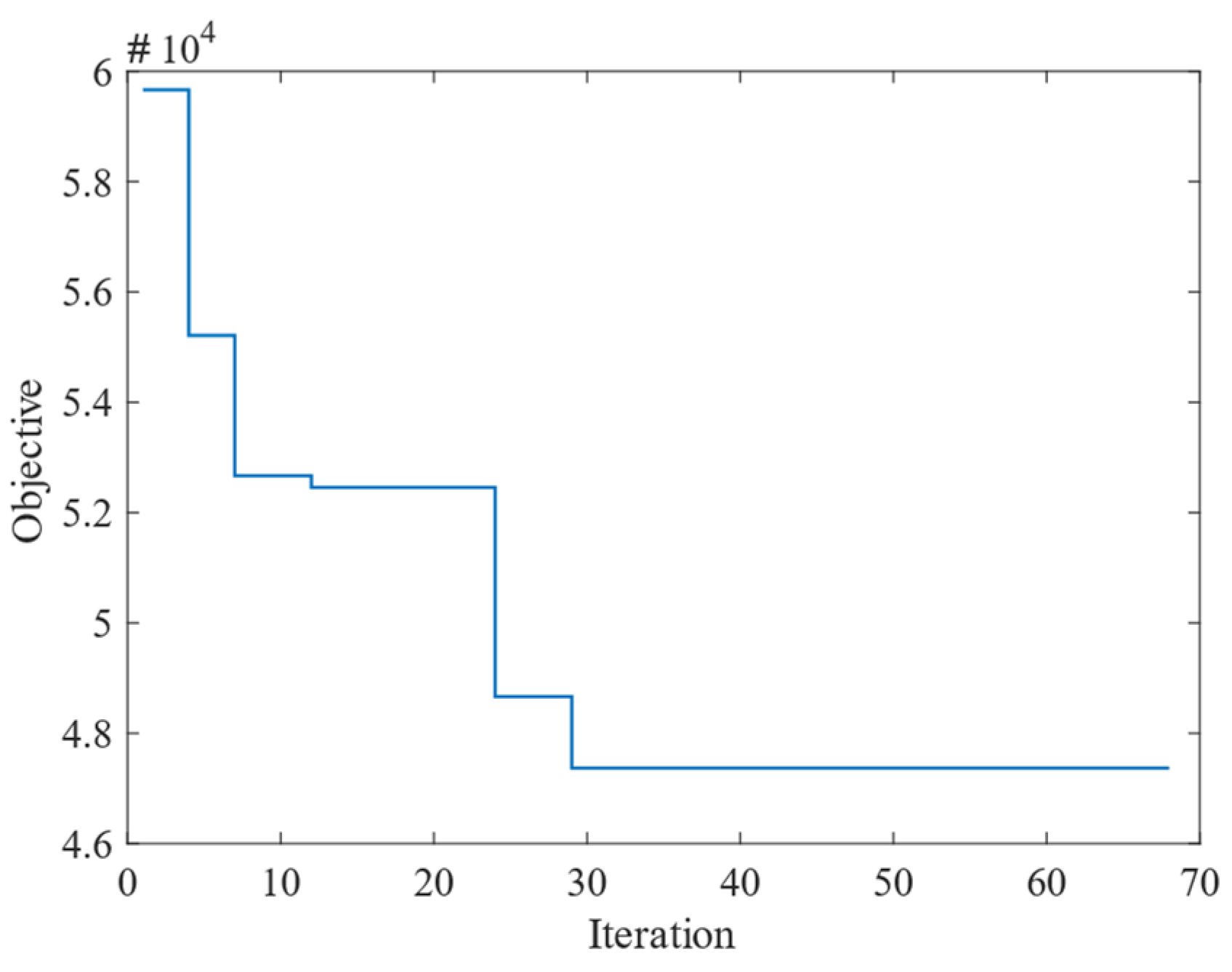
5. Algorithm Design Based on Lagrange Relaxation Decomposition

The core idea of the Lagrange relaxation decomposition algorithm is to obtain the relaxed solution and the feasible solution in each iteration. Specifically, it should firstly solve the Lagrangian relaxed model RM to obtain a relaxed solution corresponding to a lower bound and then use it to generate a feasible solution corresponding to an upper bound. With the Lagrangian multipliers improved by iterations, both the lower and upper bound will be continuously improved. The iteration process terminates until the gap between these two bounds is less than or equal to the given acceptable value or the iteration number reaches the maximum given value. The basic idea and the framework of the Lagrange relaxation decomposition algorithm are introduced in Section 5.1. Furthermore, the algorithms that generate the relaxed and the feasible solutions are detailed in Section 5.2 and Section 5.3, respectively, which are the most critical parts of the algorithm.

5.1. The Solving Framework of Lagrange Relaxation Decomposition Algorithm

We obtain the lower bound by solving each Lagrangian relaxation sub-model SRM of the RM model in each iteration. Since the lower bound can be optimized by the Lagrangian multipliers, we use the Lagrangian multipliers as the decision variables to construct a dual model called DM, as follows:

$$\underset{\mu ,\beta ,\gamma ,\omega }{\max }L=\underset{x}{\min }{\displaystyle \sum }_f{\displaystyle \sum }_{a\in \mathrm{A}}{x}_f\left(a\right)·L\left(a\right)-{\displaystyle \sum }_f{\displaystyle \sum }_h{\displaystyle \sum }_{m\to n}{\displaystyle \sum }_{t\in h_t}{\vartheta }_{m,n}^f\left(t\right)·{\omega }_{m,n}^h+ℱ$$

(20)

$$\mathrm{s}.\mathrm{t}.\hspace{1em}{\mu }_k\ge 0,\hspace{1em}\forall k|{\mathrm{y}}_k\in S_y$$

(21)

$${\beta }_{k,k^{\prime }}^t\ge 0,\hspace{1em}\forall \left(k,k^{\prime }\right)\in E;t=0,1,\cdots ,T$$

(22)

$${\gamma }_{k,k^{\prime }}^t\ge 0,\hspace{1em}\forall \left(k,k^{\prime }\right)\in E;t=0,1,\cdots ,T$$

(23)

$${\omega }_{m,n}^h\ge 0,\hspace{1em}\forall m\to n;\forall h$$

(24)

We can solve the above dual model DM of the relaxation model to obtain the optimal relaxed solution corresponding to the optimal lower bound. The sub-gradient method is widely used to solve the dual problem of Lagrangian relaxation. For example, Xu et al. [23] designed an improved sub-gradient algorithm to solve the Lagrangian relaxation problem of the joint optimization of train scheduling and locomotive allocation. Castillo et al. [24] proposed the stepwise sub-gradient method based on the standard sub-gradient algorithm to improve the convergence speed of solving dual problems. The core idea of the sub-gradient method in our problem is given as follows.

The sub-gradients of the $n$ iteration are represented as ${\rho }_{\mu }^n\left(k\right),{\rho }_{\beta }^n\left(t,k,k^{\prime }\right)$, ${\rho }_{\gamma }^n\left(t,k,k^{\prime }\right)$ and ${\rho }_{\omega }^n\left(m,n\right)$, respectively, and they can be updated as follows:

$${\rho }_{\mu }^n\left(k\right)={\displaystyle \sum }_f{\displaystyle \sum }_{t=0}^T{x}_f\left({\hat{a}}_k^t\right)-{\displaystyle \sum }_f{\displaystyle \sum }_{t=0}^T{x}_f\left({\check{a}}_k^t\right)$$

(25)

$${\rho }_{\beta }^n\left(t,k,k^{\prime }\right)={\displaystyle \sum }_f{\displaystyle \sum }_{\tau =t}^{t+\Delta D-1}{\displaystyle \sum }_{{\tilde{a}}_{k,k^{\prime }}^{\tau ,{\tau }^{\prime }}\in D{A}_{k,k^{\prime }}^{\tau }}{x}_f\left({\tilde{a}}_{k,k^{\prime }}^{\tau ,{\tau }^{\prime }}\right)-1$$

(26)

$${\rho }_{\gamma }^n\left(t,k,k^{\prime }\right)={\displaystyle \sum }_f{\displaystyle \sum }_{\tau =t}^{t+\Delta A-1}{\displaystyle \sum }_{{\tilde{a}}_{k,k^{\prime }}^{{\tau }^{\prime },\tau }\in A{A}_{k,k^{\prime }}^{\tau }}{x}_f\left({\tilde{a}}_{k,k^{\prime }}^{{\tau }^{\prime },\tau }\right)-1$$

(27)

$${\rho }_{\omega }^n\left(m,n\right)=L_{m,n}^{h_t}-{\displaystyle \sum }_f{\displaystyle \sum }_{t\in h_t}{\vartheta }_{m,n}^f\left(t\right)$$

(28)

According to the updated sub-gradients, four Lagrange multipliers of the $n+1$ iteration are updated as follows:

$${\mu }_k{}^{\left(n+1\right)}=max\left\{0,{\mu }_k{}^{\left(n\right)}+g^n·{\rho }_{\mu }^n\left(k\right)\right\}$$

(29)

$${\beta }_{k,k^{\prime }}^t{}^{\left(n+1\right)}=max\left\{0,{\mu }_k^{\prime }{}^{\left(n\right)}+g^n·{\rho }_{\beta }^n\left(t,k,k^{\prime }\right)\right\}$$

(30)

$${\gamma }_{k,k^{\prime }}^t{}^{\left(n+1\right)}=max\left\{0,{\mu }_k^{\prime }{}^{\left(n\right)}+g^n·{\rho }_{\gamma }^n\left(t,k,k^{\prime }\right)\right\}$$

(31)

$${\omega }_{m,n}^{\left(n+1\right)}=max\left\{0,{\mu }_k^{\prime }{}^{\left(n\right)}+g^n·{\rho }_{\omega }^n\left(m,n\right)\right\}$$

(32)

where ${\mu }_k{}^{\left(n\right)}, {\beta }_{k,k^{\prime }}^t{}^{\left(n\right)}$, ${\gamma }_{k,k^{\prime }}^t{}^{\left(n\right)}$, ${\omega }_{m,n}^{\left(n\right)}$ are the values of Lagrangian multipliers of the $n$ iteration, respectively. $g^n$ is the step size of $n$ generation, and it is calculated as follows:

$$g^n=1/\left(1+n\right)$$

(33)

At the beginning of each iteration, the Lagrangian cost of each arc will be reset based on the current Lagrange multipliers. Since each relaxation sub-model SRM is actually a shortest path problem, we will search for the shortest rolling stock path in the time-space network with the goal of the minimum total Lagrangian cost of arcs (i.e., the optimal objective value of the sub-model SRM). Then a relaxed solution can be obtained and its corresponding lower bound is denoted as $R_{lower}^n$. After that, to ensure the rolling stock routes do not violate the constraints related to multiple rolling stock units, we change the relaxed solution to a feasible solution and denote its corresponding upper bound as $R_{upper}^n$.

After generating the relaxed solution and the feasible solution, the Lagrangian cost of each arc will be recalculated with the Lagrangian multiples updated according to formulation (29) to (32). The procedure then goes to the next iteration and terminates only when each of the following three termination conditions is triggered:

(1)

The iteration number reaches its maximum limit $N_{max}$.

(2)

All sub-gradients are no more than the given standard values ${\rho }_{max}$.

(3)

The number of continuous iterations without improving the lower bound reaches the maximum limit $K_{max}$, where the judgment principle of the unimproved lower bound is as follows:

$$\frac{\left|R_{lower}^n-R_{lower}^{n-1}\right|}{R_{lower}^{n-1}}\le \mathsf{\epsilon }$$

(34)

where $R_{lower}^n$ and $R_{lower}^{n-1}$ are the lower bounds of the $n$ and $n-1$ iterations, respectively, and ε is the given calculation accuracy.

Overall, the entire procedure of the algorithm based on the Lagrange relaxation decomposition method are shown in Algorithm 1.

Algorithm 1: Algorithm based on Lagrange relaxation decomposition

Input: rail line, number of rolling stock, set of alternative stop plans Output: Optimal feasible solution and its upper bound Start   Step 1: Initialization   Let iteration index $n=1$, initial multiplier update step size $g^n=1/2$, Lagrangian multipliers ${\mu }_k{}^{\left(n\right)}=0,{\beta }_{k,k^{\prime }}^t{}^{\left(n\right)}=0,{\gamma }_{k,k^{\prime }}^t{}^{\left(n\right)}=0,{\omega }_{m,n}^{\left(n\right)}=0$.   Step 2: Calculate the Lagrangian cost $L\left(a\right)$ and $C_q\left(f\right)$ according to formulations (16) and (17), respectively.   Step 3: (Solving the relaxation model RM to achieve a relaxed solution and its lower bound)   Achieve a relaxed solution using the relaxation solution generation sub-algorithm introduced in Section 5.2. Search the shortest paths for rolling stock based on the Lagrange cost of arcs one by one in any order.   Step 4: (Generating a feasible solution and its upper bound based on the relaxed solution)Achieve a feasible solution using the feasible solution generation sub-algorithm introduced in Section 5.3. Search the shortest paths for rolling stock based on the weights of arcs one by one in ascending priority order.   Step 5: The sub-gradient is updated according to formulations (25) to (28).   Step 6: (Termination conditions)   If all termination conditions are not satisfied, then update the Lagrange multipliers according to formulations (29) to (32), and return to step 2. Otherwise, the procedure is terminated. End

Note that the above designed algorithm includes two key sub-algorithms. One is to search for the shortest rolling stock paths without considering the constraints related to multiple rolling stock units, and the other is the heuristic algorithm to search the rolling stock paths considering constraints related to multiple rolling stock units. These two sub-algorithms are introduced in detail in Section 5.2 and Section 5.3, respectively.

5.2. Sub-Algorithm of Generating the Relaxed Solution

In this section, a shortest path algorithm based on the label strategy of the Dijkstra algorithm is designed to search the path with the minimum total Lagrangian cost for each rolling stock unit. Thus, we can obtain a relaxed solution of the model RM. Its value is the total Lagrangian costs of rolling stock paths. It should be noted that the path of each rolling stock unit will not be affected by other rolling stock paths as we do not consider the association constraints among rolling stock units in this sub-algorithm.

This sub-algorithm takes the dwell arc and the sub-path unit formed between two terminal stations of the rail line as the search object. To be exact, it starts from the virtual origin node and continuously searches for the sub-path units and dwell arcs visited by the rolling stock unit until it reaches the virtual end node. Note that we define a sub-path unit to describe the rolling stock path from one terminal station to another terminal station of the rail line. Particularly, each sub-path unit is uniquely determined by a stop plan, and a set of candidate stop plans are determined in advance. The introduction of the sub-path unit can greatly improve the searching efficiency of the shortest path and ensure the rationality of a train’s stops. In this way, we can select one of the candidate stop plans to determine the corresponding sub-path unit.

In general, the search object of the common Dijkstra shortest path algorithm is a directed arc starting from the current node, but the search object of our sub-algorithm includes both the directed arc and the sub-path unit. For the convenience of expression, the directed arc search is also regarded as a sub-path unit. Therefore, the sub-algorithm can be described as starting from the virtual origin node and continuously searching the sub-path units until reaching the virtual end node.

Based on the above main idea, a label set is defined for each node. Each label contains the information of the total cost of the shortest path from the virtual origin node to its corresponding node, its previous sub-path unit and its previous label set. Then, a shortest rolling stock path search algorithm based on the labeling idea is constructed. The symbols used in the sub-algorithm are shown in

Table 4. Symbols used in the algorithm definition.

Symbols	Meaning
$L_v$	Set of labels of node $v$
$l$	The index of label, $l\in L_v$
$v_l$	Node to which label $l$ belongs, if $l\in L_v,v_l=v$
$t_v$	Time of node $v$
$S_v$	Station to which node $v$ belongs
$Z_l$	Total Lagrangian costs for the path from virtual starting point $\overline{o}$ to node $v_l$ belonging to label $l$
${\stackrel{⟵}{l}}_l$	Pre-label of label $l$
$p\left(v,v^{\prime },q\right)$	Sub-path unit from node $v$ to node $v^{\prime }$ by stop plan $q$
$C_l\left(v,v^{\prime },q\right)$	Total Lagrangian costs of directed arcs in a path unit
$C_q$	Total cost of the $OD$ served by stop plan $q$
$L_c$	Set of labels have been checked
$L_X$	Set of labels have been checked by the latest updating
$L_{temp}$	Set of temporary storing labels

, and its detailed steps are described in Algorithm 2.

Algorithm 2: Single rolling stock shortest path search algorithm based on label idea

Input: operation time $T$, node set, arc set, number of rolling stock, candidate stop plan set, stop time parameters, turnaround time parameters Output: Relaxation solution and its upper bound Start   Step 1: Initialization    Add label $l$ to set $L_{\overline{o}}$ and let other label sets equal to $\varnothing$.    Let set $L_c=L_X=\left\{l\right|v_l=\overline{o}\}$, set $L_{temp}=\varnothing .$   Step 2: Label checking and updating    Select each label $l$ in set $L_X$ one by one, execute     Select sub-path units $p\left(v,v^{\prime },q\right)$ from node $v_l$ of label $l$ one by one, and execute      If $l^{\prime }=\varnothing$, execute        Add the label $l^{\prime }$ to label set $L_{v^{\prime }}$ of the node $v_{l^{\prime }}$, and set its subordinate nodes $v_{l^{\prime }}=v^{\prime }$, total cost       $Z_{l^{\prime }}=+\infty$ and pre-label ${\stackrel{⟵}{l}}_{l^{\prime }}=\varnothing$.      If $l^{\prime }\notin L_c$, execute        If the time of the nodes contained in sub-path unit $p\left(v,v^{\prime },q\right)$ are all within the operation time $T$, execute         Calculate the total cost $C_l\left(v,v^{\prime },q\right)$ of the sub-path unit and the OD service cost $C_q$ of the stop plan.      If $Z_{l^{\prime }}>Z_l+C_l\left(v,v^{\prime },q\right)-C_q$, execute      Let $Z_{l^{\prime }}=Z_l+C_l\left(v,v^{\prime },q\right)-C_q$, ${\stackrel{⟵}{l}}_{l^{\prime }}=l$, and add label $l^{\prime }$ to set $L_{temp}$.   Step 3: Judgment termination condition    Let $L_X=\varnothing$. Find the minimum cost label in $L_{temp}$ and transfer it to $L_c$ and $L_X.$     If there is label $\overline{l}$ in $L_X$ and its node $v_{\overline{l}}$ is the virtual end point $\overline{d}$, go to step 4. Otherwise, return to step 2.   Step 4: Backtracking primary path and determining all subordinate paths    Traceback the path from node $v_{\overline{l}}$ of label $\overline{l}$ according to the node and the path unit of pre-label End

5.3. Sub-Algorithm of Generating Feasible Solution Based on the Relaxed Solution

This sub-algorithm is to obtain a feasible solution based on a relaxed solution, to make it satisfy the constraints related to multiple rolling stock units such as safe headway, maintenance requirements, and OD service frequency requirements. Note that the rolling stock path with the lower total Lagrangian cost in the relaxed solution contains more non-dwell arcs, which is more conducive to improving the objective value of the model EM. Thus, we rank the rolling stock units in ascending order according to their optimal objective values of the sub-model SRM. Then, search the path for each rolling stock unit one by one in this order. In order to ensure the train scheduling does not violate the constraints (9 to12) related to multiple rolling stock units of the equivalent model BM, the occupied arcs by the former paths cannot be chosen by the current rolling stock unit.

Compared with the sub-algorithm generating the relaxation solution, the sub-algorithm generating feasible solution has the following differences.

• Path search is based on the total weights of arcs contained in each path unit. To be exact, it aims to find the path with the minimum total weights of arcs, rather than the path with the minimum total Lagrangian cost of arcs. For simplicity, the symbols $Z_l$ and $C_l\left(v,v^{\prime },q\right)$ in this section are redefined as the total weights of arcs.
• In order to satisfy the OD service frequency constraints, there are two options when searching a path for the current rolling stock unit. If the generated rolling stock paths have not satisfied the minimum service frequency requirements of each OD, it will select the sub-path unit that is most conductive to improving the OD service frequency according to the greedy principle. Otherwise, when all OD service frequencies in the generated paths have met the requirements, it will select the sub-path unit with the minimum number of stops (i.e., the sub-path unit with minimum total weights of arcs). The matching degree $c_{od}$ of service OD of each stop plan is calculated as follows:

  $$c_{od}=\{\begin{array}{cc}1 ,& if {\displaystyle \sum _h}{\displaystyle \sum _{o\to d}}{\displaystyle \sum _{t\in h_t}}{\vartheta }_{o,d}^f\left(t\right)<L_{o,d}^{h_t}\\ 0.1 ,& if {\displaystyle \sum _h}{\displaystyle \sum _{o\to d}}{\displaystyle \sum _{t\in h_t}}{\vartheta }_{o,d}^f\left(t\right)\ge L_{o,d}^{h_t}\end{array}$$

  (35)
• In order to satisfy constraints on arrival and departure intervals related to multiple rolling stock units, the restricted arc set is determined in advance. No arcs in the set are allowed to be selected, otherwise the safe headway conflict will occur. The restricted arc set consists of running arcs that are occupied by high priority rolling stock units and the related running arcs that do not conform to their safe interval constraints. Let $A_{visit}$ be denoted as the set of all running arcs selected by the scheduled rolling stock paths, then restrict arc set. $A_{restrict}$ can be determined as follows:

  $$A_{restrict}=A_{visit}\cup \left\{{\tilde{a}}_{k,k^{\prime }}^{\tau ,{\tau }^{\prime }}|\exists {\tilde{a}}_{k,k^{\prime }}^{t,t^{\prime }}\in A_{visit},\left|t-\tau \right|<\Delta D\right\}\cup \left\{{\tilde{a}}_{k,k^{\prime }}^{{\tau }^{\prime },\tau }|\exists {\tilde{a}}_{k,k^{\prime }}^{t^{\prime },t}\in A_{visit},\left|t-\tau \right|<\Delta A\right\}$$

  (36)
• In order to meet the rolling stock maintenance constraint we must ensure that all rolling stock units can enter the maintenance depot within 48 h. Thus, for each rolling stock unit, if it starts from the virtual leave-arc related to the maintenance depot, it can choose any virtual entry-arc to return to the virtual end node. Otherwise, it can only return to the virtual end point by the virtual entry-arc related to the maintenance depot. In this way, we can guarantee that all rolling stock units stay one night every two days at the maintenance depot to receive maintenance.

In summary, based on the sub-algorithm generating relaxation solution, the sub-algorithm generating a feasible solution can be designed by integrating the differences of the path search above, and its detailed steps are described in Algorithm 3.

Algorithm 3: Heuristic algorithm for generating feasible solutions

Input: operation time $T$, node set, arc set, number of rolling stock, candidate stop plan set, dwell time parameters, turnaround time parameters Output: Feasible solution and upper bound Start   Step 1: Initialization   Let $A_{restrict}=\varnothing$. Rank all rolling stock in ascending order according to their optimal function value in model SRM.    The priority order is represented as $f_{\left(n\right)}$.   Step 2: Search rolling stock path one by one   Select rolling stock $f$ in priority order $f_{\left(n\right)}$, execute    Step 2.1: Initialization    Add label $l$ to set $L_{\overline{o}}$ and let other label sets equal to $\varnothing$.    Let $L_c=L_X=\left\{l\right|v_l=\overline{o}\}$, $L_{temp}=\varnothing .$    Step 2.2: Judging the balance between entering and leaving the depot    Judge whether the rolling stock starting from the depot with maintenance capability can return to the depot and adjust the virtual arc of returning to the depot.    Step 2.3: Restricted arc set updating      Update $A_{restrict}$ according to the restricted arc set update method.    Step 2.4: Label checking and updating    Select each label $l$ in the set $L_X$ one by one, execute     Select sub-path units $p\left(v,v^{\prime },q\right)$ from node $v_l$ of label $l$ one by one, execute      If the sub-path unit is not a dwell arc, execute       The combination of greedy principle and shortest path principle is used to select the optimal sub-path unit for node $v_l$.      If $l^{\prime }=\varnothing$, execute        Add the label $l^{\prime }$ to the label set $L_{v^{\prime }}$ of node $v_{l^{\prime }}$, and let $v_{l^{\prime }}=v^{\prime }$, $Z_{l^{\prime }}=+\infty$, ${\stackrel{⟵}{l}}_{l^{\prime }}=\varnothing$.       If $l^{\prime }\notin L_c$, execute        If the time of the nodes contained in $p\left(v,v^{\prime },q\right)$ is within the time $T$, execute       Calculate the total cost $C_l\left(v,v^{\prime },q\right)$ of the sub-path unit.        If $Z_{l^{\prime }}>Z_l+C_l\left(v,v^{\prime },q\right)$, execute          let $Z_{l^{\prime }}=Z_l+C_l\left(v,v^{\prime },q\right),{\stackrel{⟵}{l}}_{l^{\prime }}=l$, and add $l^{\prime }to{L}_{temp}$.    Step 2.5: Termination conditions    Let $L_X=\varnothing$. Find the label with the lowest cost in $L_{temp}$ and transfer it to $L_c$ and $L_X$.    If $\overline{l}\in L_X$ and node $v_{\overline{l}}$ is node $\overline{d}$, go to Step 2.6. Otherwise, return to Step 2.4.    Step 2.6: Backtracking primary path and determining all subordinate paths    Traceback the path from node $v_{\overline{l}}$ of label $\overline{l}$ according to the node and the sub-path unit of pre-label. End

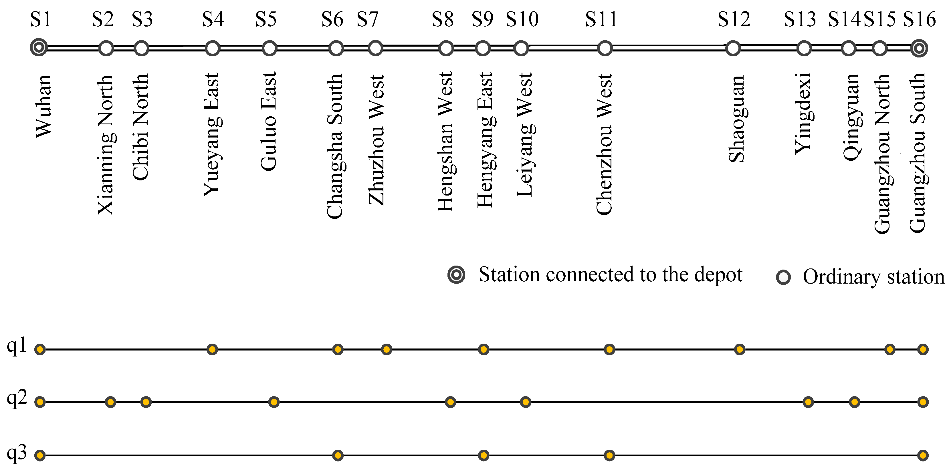
6. Case Study

In this section, we conduct a computation study on a practical double-track high-speed railway line to test the performance of this algorithm. We show the results of the solution and perform an in-depth analysis of them.

6.1. Experiment Setup

In this case study, the performance of our approach is reported on a practical high-speed railway between Wuhan city and Guangzhou city in China. This high-speed railway consists of 16 stations and 15 double-track rail sections, and its total length is 1069 km, as shown in Figure 5. Its terminal stations, namely Wuhan station and Guangzhou South station, have the turnaround capacity, and they both connect to the maintenance depots. We define the direction of leaving from Wuhan station as the downward direction, and the direction of leaving from Guangzhou South station as the upward direction.

We set the parameters of the stop plans and the OD service frequency according to the passenger flow characteristics and train plan in this railway in 2016. The planning horizon T is set from 6:00 to 24:00. We divide it into three time periods according to passenger travel preferences, namely [6:00–10:00], [10:00–16:00], [16:00–24:00]. Particularly, we set time period 2 (i.e., from 10:00 to 16:00) as a high demand period, because passengers prefer to travel during this period. The parameters of all OD service frequency in the whole day are shown in

Table 5. The parameters of all OD service frequency in the whole day.

OD	S1	S2	S3	S4	S5	S6	S7	S8	S9	S10	S11	S12	S13	S14	S15	S16
S1	0	27	27	40	27	53	40	27	53	27	53	40	27	27	40	53
S2	27	0	27	0	27	0	0	27	0	27	0	0	27	27	0	27
S3	27	27	0	0	27	0	0	27	0	27	0	0	27	27	0	27
S4	40	0	0	0	0	40	40	0	40	0	40	40	0	0	40	40
S5	27	27	27	0	0	0	0	27	0	27	0	0	27	27	0	27
S6	53	0	0	40	0	0	40	0	53	0	53	40	0	0	40	53
S7	40	0	0	40	0	40	0	0	40	0	40	40	0	0	40	40
S8	27	27	27	0	27	0	0	0	0	27	0	0	27	27	0	27
S9	53	0	0	40	0	53	40	0	0	0	53	40	0	0	40	53
S10	27	27	27	0	27	0	0	27	0	0	0	0	27	27	0	27
S11	53	0	0	40	0	53	40	0	53	0	0	40	0	0	40	53
S12	40	0	0	40	0	40	40	0	40	0	40	0	0	0	40	40
S13	27	27	27	0	27	0	0	27	0	27	0	0	0	27	0	27
S14	27	27	27	0	27	0	0	27	0	27	0	0	27	0	0	27
S15	40	0	0	40	0	40	40	0	40	0	40	40	0	0	0	40
S16	53	27	27	40	27	53	40	27	53	27	53	40	27	27	40	0

For simplicity, the stations are numbered in sequence in the down direction, corresponding to S1–S16.

and the parameters in each time period are set according to the ratio of 3:8:3. There are three candidate stop plans, as shown in Figure 5.

In this case, both the minimum departure and arrival time intervals in rail sections are set as 5 min. The minimum and the maximum dwell times at each station are set as 3 min and 5 min, respectively. The minimum turnaround time is set as 20 min. The additional times for the decelerating and accelerating are both 1 min. The minimum running times are set as shown in

Table 6. The minimum running times.

Section	Origin Station	Terminal Station	Minimum Running Time (min)
1	Wuhan	Xianning North	20
2	Xianning North	Chibi North	10
3	Chibi North	Yueyang East	21
4	Yueyang East	Guluo East	17
5	Guluo East	Changsha South	18
6	Changsha South	Zhuzhou West	12
7	Zhuzhou West	Hengshan East	20
8	Hengshan East	Hengyang East	10
9	Hengyang East	Leiyang West	13
10	Leiyang West	Chenzhou West	24
11	Chenzhou West	Shaouguan	36
12	Shaouguan	Yingdexi	21
13	Yingdexi	Qingyuan	14
14	Qingyuan	Guangzhou North	9
15	Guangzhou North	Guangzhou South	11

. In addition, the parameters related to the algorithm are shown in

Table 7. Values of parameters in algorithm.

Parameter	Value	Unit
$T$	1080	min
$h$	[1–239; 240–599, 600–1080]	min
$Q_h$	[$q_1{q}_2{q}_3;q_1{q}_2{q}_3;q_1{q}_2{q}_3$]	-
$N_{max}$	100	-
${\rho }_{max}$	0.05	-
$K_{max}$	20	-
$\mathsf{\epsilon }$	0.005	-

.

All algorithms are implemented by a Matlab 9.1.0.441655 (R2016b) version and all instances are performed on a XiaoXinAir-14ARE 2020 Laptop with a 2.10 GHz CPU, 16.0 GB memory (15.4 GB usable) and a Windows 10 64-bit professional operating system.

6.2. Analysis with the Computational Results

In the following case studies, we define the following evaluation indexes to evaluate the quality of the solution.

• Upper bound (UB): the optimal objective value of model EM. This corresponds to a feasible solution.
• Trans scheduled: the maximum number of trains that can be included in the train timetable.
• Capacity utilization (CU): indicating the transportation capacity in a train timetable which is the ratio of the number of scheduled trains to the ideal number of trains.

Note that the number of scheduled trains in the train timetable corresponds to an optimal feasible solution, and the ideal number of trains refers to the upper limit of railway capacity. Considering that the dwell time and the number of stops will affect the departure intervals among trains, it is generally impossible to achieve the capacity calculated by the minimum safe headway. Thus, we calculate the ideal number of trains with a deduction coefficient based on the actual operation experience, and its formulation as follows:

$$\mathrm{Ideal}\mathrm{number}\mathrm{of}\mathrm{trains}=\frac{T-T_o}{\Delta D}\times \left(1-ℛ\right)\times 2\times 100\%$$

(37)

where, $\Delta D$ represents the minimum departure interval as well as the minimum safe headway. $T_o$ represents fixed occupied time, and it is set as $T_o=212$. $ℛ$ represents the deduction coefficient, and it is set as $ℛ=0.1$.

6.2.1. Computational Results

Table 8. Computation results with increasing values of $\left|L\right|$.

$\left|\mathit{L}\right|$	UB	Trains Scheduled	CU
80	33,400	250	80.01%
84	35,176	262	83.85%
88	36,952	274	87.69%
92	39,576	282	90.25%
96	43,048	286	91.53%
100	47,368	286	91.53%
120	68,968	286	91.53%

shows part of the optimization results when the input number of rolling stock units is increased from 80 to 120, and $\left|L\right|$ represents the input amount of rolling stock units. Based on the results, we can observe that the maximum number of scheduled trains in the practical high-speed railway is 286, and the actual number of used rolling stock units is 95. As the optimal result, no more trains can be added to the train timetable, and the capacity utilization rate is up to 91.53%. It shows that our approach can effectively improve transportation capacity.

Figure 6 shows the convergence process of the Lagrangian algorithm when $\left|L\right|=100$. The algorithm terminates after 68 iterations, and it can stably converge. The train timetable obtained by this algorithm is shown in Figure 7.

6.2.2. Analysis of the Turnaround Efficiency of Rolling Stock

The turnaround time of a rolling stock unit determines its turnaround efficiency. Figure 8 shows the number of trains served by a rolling stock unit and the average time for one turnaround. As shown, there are 95 rolling stock units in service. We observe that a rolling stock unit with a shorter turnaround time can serve more trains. There are 67 rolling stock units whose turnaround times are within 40 min, accounting for 70%. The number of rolling stock units serving 4 trains is 10, and their average turnaround time is about 20 min, which is equal to the minimum turnaround time. This indicates that the connection efficiency of rolling stock is extremely high. The number of rolling stock units serving 3 trains is 78, and their average turnaround time is 33 min. The number of rolling stock units serving 2 trains is 5, and their average turnaround time is 69 min, which is relatively long but acceptable. Besides, there are 2 rolling stock units that only serve one train, so there is no turnaround process. In general, the turnaround times of rolling stock are short or acceptable, and the turnaround efficiency is high.

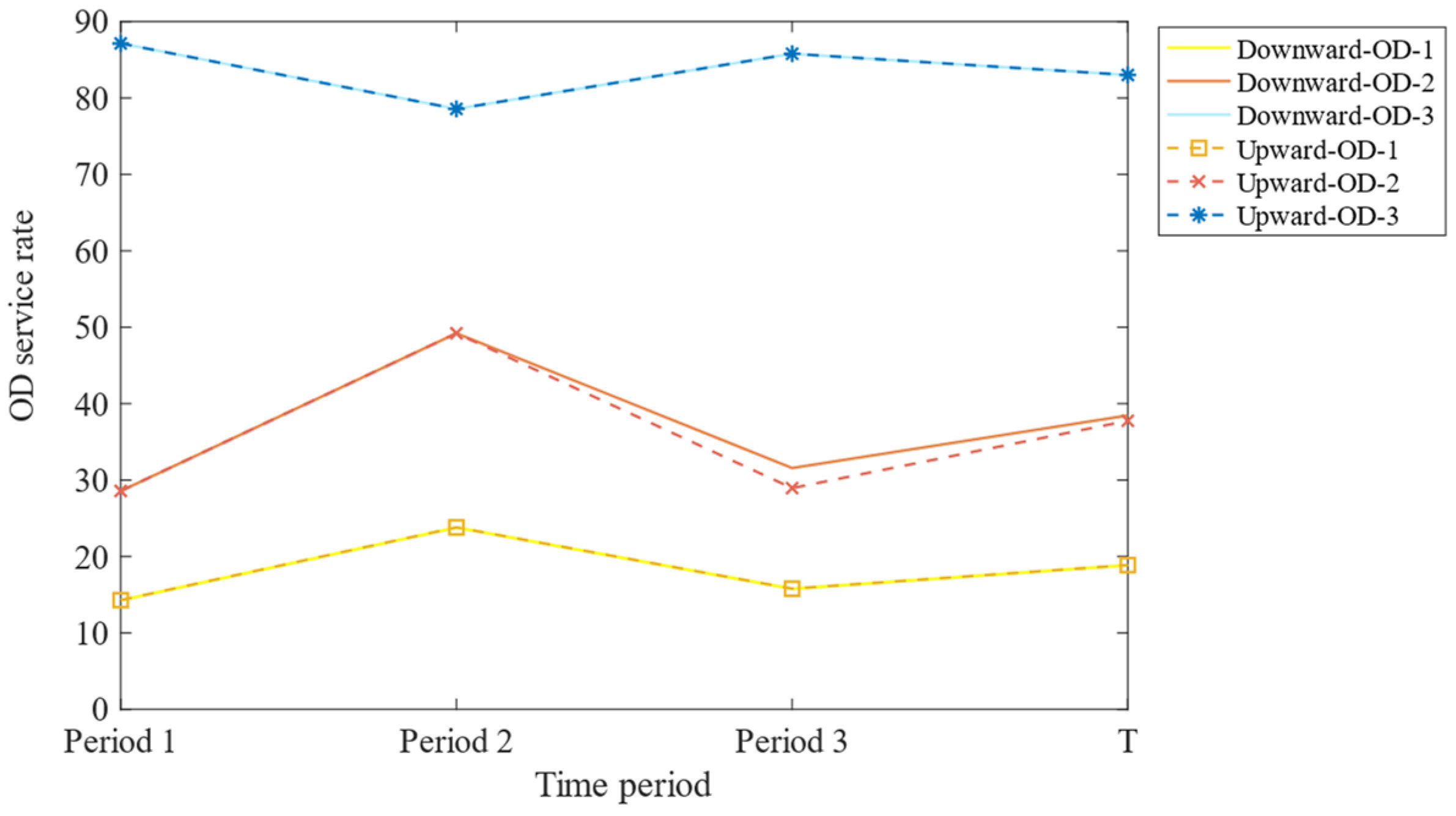
6.2.3. Analysis of OD Service Quality

In order to explore the influence of different OD demand intensities on train scheduling, we divide the planning time into three time periods. Each time period has different OD service requirements. In particular, time period 2 is the high demand period. According to the different travel demand intensities, we set three types of ODs. These ODs are denoted as OD-1, OD-2, OD-3 in descending order of intensity, corresponding to the ODs with values of 27, 40, and 53 in

Table 9. OD service frequency.

Direction	Type	Time Period 1		Time Period 2		Time Period 2		$$\mathit{T}$$
		Minimum Value	Average Value	Minimum Value	Average Value	Minimum Value	Average Value	Minimum Value	Average Value
Downward	OD-1	6	6	15	15	6	6	27	27
	OD-2	9	12	23	31	9	12	40	55
	OD-3	11	37	30	50	11	33	53	119
Upward	OD-1	6	6	15	15	6	6	27	27
	OD-2	9	12	23	31	9	11	40	54
	OD-3	11	37	30	50	11	33	53	119

, respectively.

Table 9 shows the service frequency of each OD in different time periods. The ‘Average value’ in the Table 9 is the average service frequency of ODs. The ‘Minimum value’ in the Table 9 indicates the minimum service frequency required by ODs. Figure 9 shows the OD service rate in upward and downward directions. The OD service rate is the ratio of the OD service frequency to the number of scheduled trains.

From Table 9, we observe that the train scheduling can satisfy the requirements of different OD service frequencies in different time periods. If the OD demand intensity is high, the OD service frequency tends to be high. This indicates that it tends to provide more train services for ODs with a large travel demand.

Figure 9 compares the OD service rates in different time periods. The minimum OD service rate of OD-3 is in period 2, and the maximum OD service rates of OD-1 and OD-2 are in period 2. It indicates that all the ODs of various travel demand intensity have satisfactory OD service rates in high demand time periods. In other time periods, trains prefer to serve ODs with a high travel demand.

Overall, our approach can provide OD services that match the OD travel demand distribution.

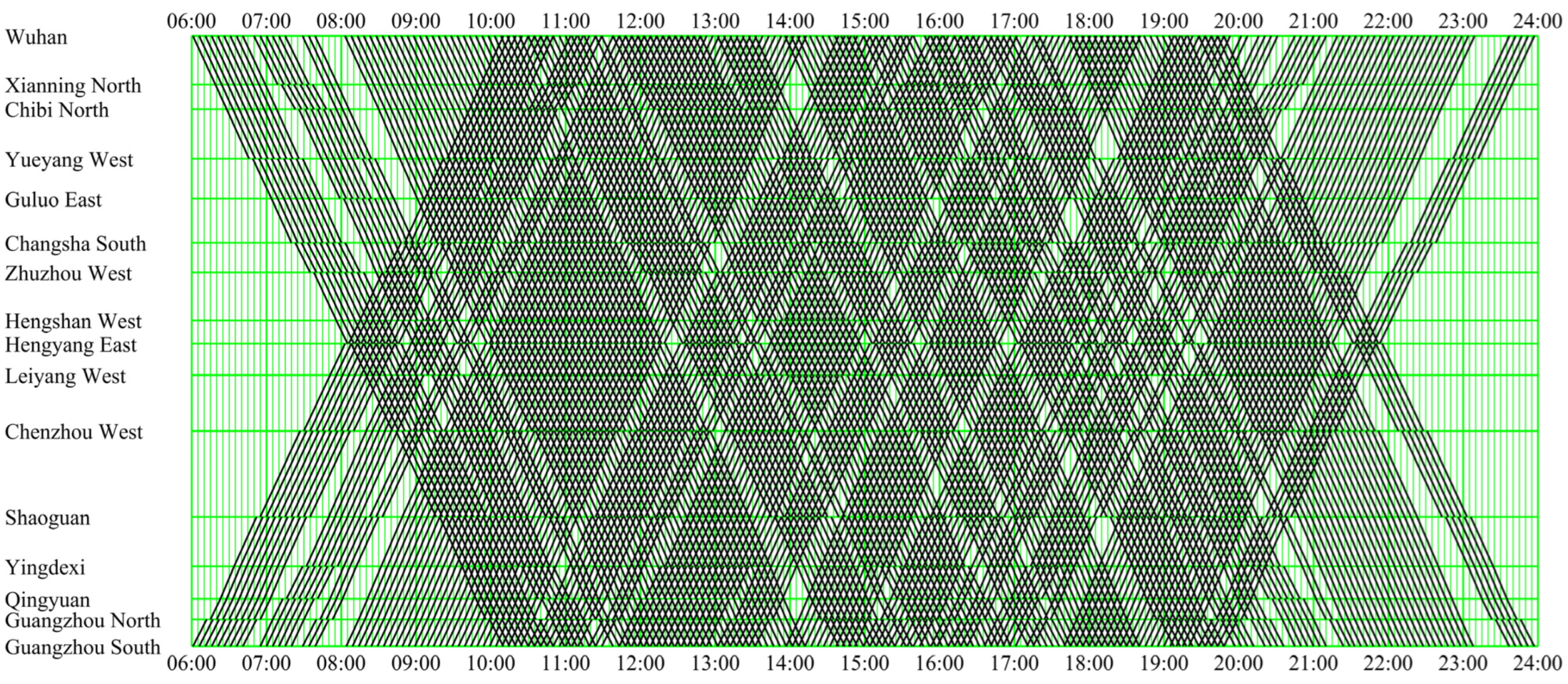
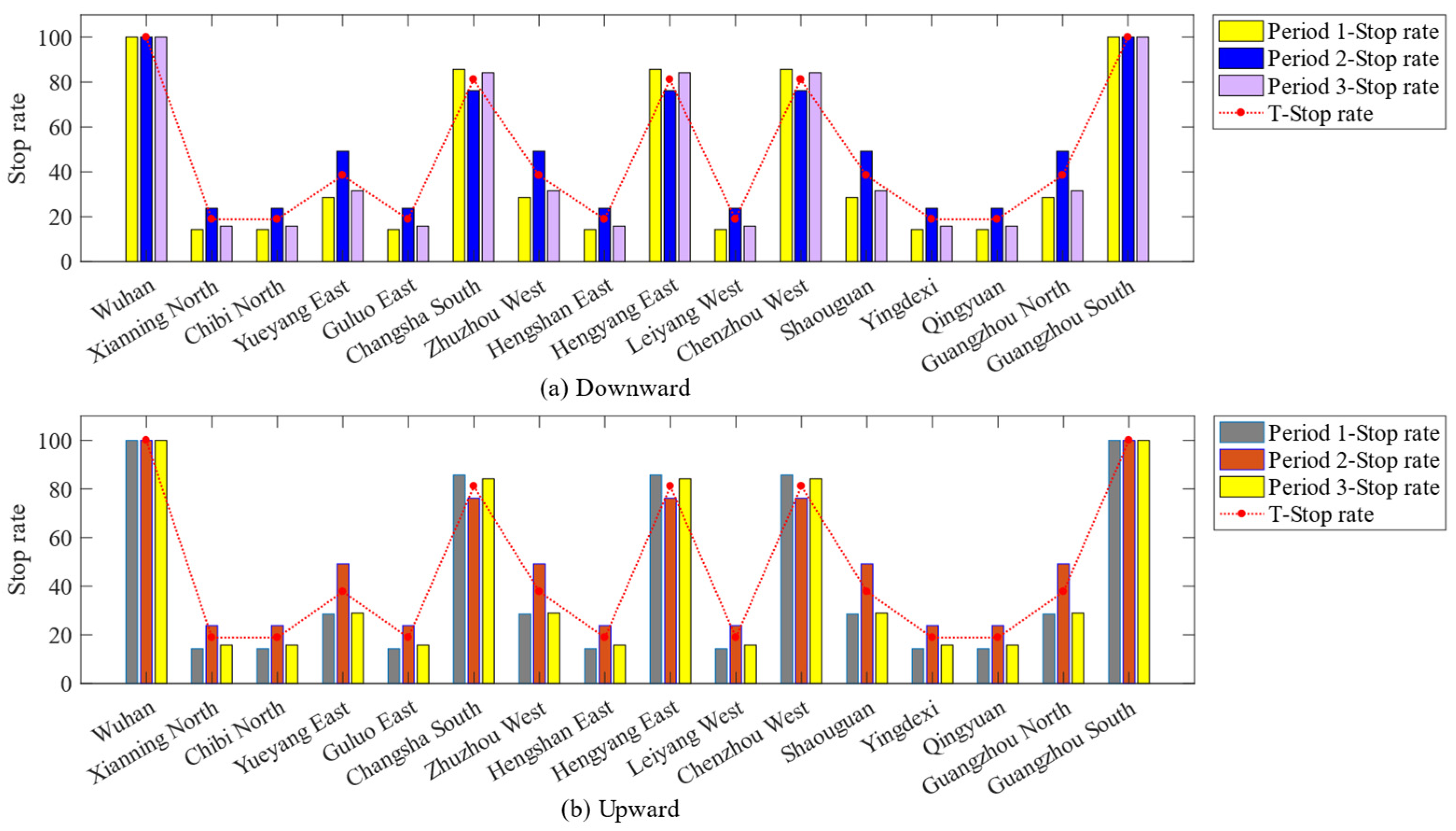
6.2.4. Analysis of the Quality of Train Services

Along the Wuhan-Guangzhou high-speed railway, there are seven intermediate stations with large passenger flow, namely Yueyang East, Changsha South, Zhuzhou West, Hengyang East, Chenzhou West, Shaoguan, and Guangzhou North. Among them, the passenger flow of Changsha South, Hengyang East and Chenzhou West is far larger than other stations. Based on the passenger flow distribution at each station, we can analyze the quality of train services from the following aspects.

Figure 10 shows the train stop rate at each station in different time periods. Comparing Figure 10a,b, it can be found that the train stop rates in the upward and downward directions have the same distribution characteristics. Comparing different time periods, we can observe that the stopping rates at each station have the same distribution characteristics. Particularly, a station with high passenger flow has a high stop rate. For example, the stop rates of Changsha South station, Hengyang East station and Chenzhou West station are 81.1%. In summary, this means that we can provide train services that match the passenger flow distribution of each station in different time periods and in different directions.

Table 10. Stop plans and average train travel time.

Stop Plan	Average Train Travel Time/min		D-Value		Number of Stop Plans
	Down Direction	Up Direction	Down Direction	Up Direction	Down Direction	Up Direction
$q_1$	249	249	0	0	55	54
$q_2$	249	249	0	0	27	27
$q_3$	229	229	0	0	61	62

shows the use of each stop plan and the corresponding average train travel time. The “D-value” column reports the difference between the average travel time and the minimum travel time. $q_1$ ensures that the train stops at large passenger flow stations. $q_2$ ensures that the train stops at small passenger flow stations. $q_3$ is the stop plan with the minimum number of stops, mainly serving the ODs among the five stations of Wuhan, Changsha South, Hengyang East, Chenzhou East, and Guangzhou North.

From Table 10, the results show that the number of q₃ and q₁ is more than the number of q₂. This indicates that the trains will choose the matching stop plans according to the passenger flow of the stations. Comparing D-value, we observe that the train travel times are short, and there is no serious operational disturbance between different trains. Therefore, trains can provide efficient transportation services.

Table 11. Time-space distribution of trains and rolling stock departure.

Origin Station	Number of Train Departures			Number of Rolling Stock Units
	Period 1	Period 2	Period 3	T	Departure	Arrival
Wuhan	42	63	38	143	48	48
Guangzhou South	42	63	38	143	47	47

shows the time-space distribution of trains. From the perspective of time distribution, the trains departing from the upward and downward directions are the same in each time period, which indicates that the train departure distribution is symmetrical. From the perspective of time distribution, the number of departures in time period 2 is more than that in the other two time periods because the transportation demand in this time period is huge. In summary, the number of trains is consistent with the trend of travel demand over time.

Furthermore, Table 11 displays the origin places and terminal places of rolling stock units. We observe that the number of rolling stock units departing and returning at each depot is equal which indicates that we can ensure the daily repeated operation of rolling stock.

6.3. Analysis of Sensitivity

The amount of rolling stock and the minimum headway are very important factors of capacity in our problem. Specifically, we conduct some instances to explore the sensitivity of transportation capacity and its impact factors with different parameters. To save the computation time of the algorithm, we construct a small-scale double-track rail line containing five stations. The planning time horizon is 240 min and the parameters of the Lagrangian algorithm are unchanged. Other time parameters are reset according to Appendix A. In this section, we will analyze the sensitivity based on this small-scale case.

6.3.1. Analysis of Sensitivity Based on Rolling Stock Amount

In order to explore the influence of the rolling stock amount on railway capacity, we set the minimum headway to 4 min and increase the number of rolling stock units from 1 to 35.

From Figure 11, we observe that there are no feasible solutions here when the $\left|L\right|$ value is less than 9. This is because the current number of rolling stock units is small, and it cannot satisfy the requirements of all OD service frequency in all time periods. As seen in it, UB increases as $\left|L\right|$ increases, because for every additional rolling stock unit, whether it is used or not, the time it stays at stations or depots is counted. Figure 11 further shows that CU value increases first and then remains unchanged as the $\left|L\right|$ value increases from 10 to 25. It indicates that increasing the number of rolling stock units can improve the transportation capacity, but there is an upper limit to it. Furthermore, it can be found that the maximum capacity utilization rate in our case is 88.89%. Its corresponding transportation capacity is very close to the upper limit of the transportation capacity.

As shown in Figure 12, the blue curve shows the variation of the number of scheduled trains with different rolling stock amounts. The ideal number of trains with the red dashed line is 99. We observe that the number of scheduled trains grows faster at the beginning as $\left|L\right|$ increases. When $\left|L\right|=16$, the rail line can schedule 80 trains, and the capacity utilization rate is 80.81%. After that, its growth gradually slows down to no change, and it reaches 88 when $\left|L\right|\ge 19$. This means that at least three rolling stock units must be added to reach the maximum transportation capacity, but the capacity utilization rate is increased by only 8%. Thus, from the point of view of saving operational cost, it is not economical to use too many rolling stock units when the transportation capacity is large enough.

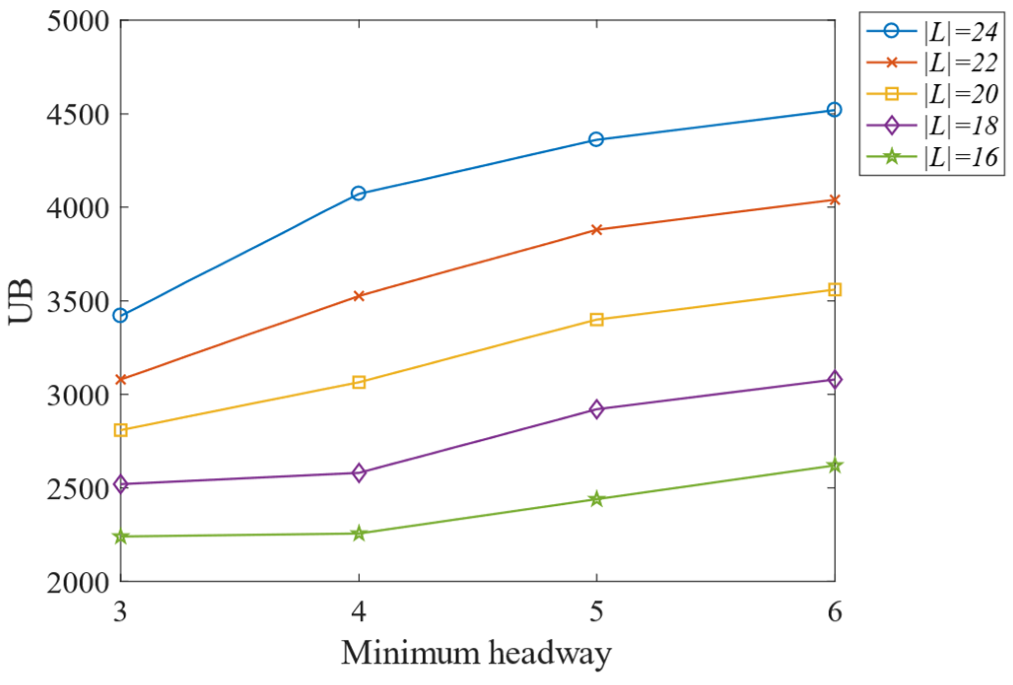
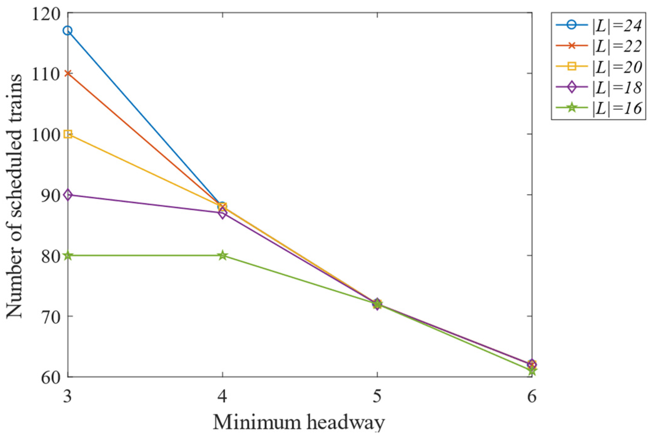
6.3.2. Analysis of Sensitivity Based on Minimum Headway

The minimum headway denoted as $\Delta D$ is an important factor affecting the railway capacity. In order to analyze the influence of different minimum headways on the results, we set $\left|L\right|=16,18,20,22,24$ and $\Delta D=3, 4, 5, 6$.

Figure 13 shows the variation tendency of UB with the increase in the minimum headway. We observe that UB value increases as $\Delta D$ increases. In addition, if the $\left|L\right|$ value is larger, the UB value is higher. This is because the increase in the minimum headway will increase the waiting time of the rolling stock units in stations or depots.

Figure 14 displays the variation of CU with the increase in the minimum headway. We observe that when the rolling stock amount is small (16 and 18 in the instance), CU increases significantly as $\Delta D$ decreases. This indicates that the increase in the minimum headway will result in a smaller upper limit of transportation capacity. However, when the rolling stock amount is large (20, 22 and 24 in the instance) and $\Delta D$ value is small, CU is significantly affected by $\left|L\right|$. As seen in it, when $\Delta D$ = 3, the CU increases from 60.61% to 88.64% with the increase of $\left|L\right|$. This is because the transportation capacity at this time is limited by the amount of rolling stock, and there is still room for further improvement. Furthermore, we also observe that the capacity utilization rate can reach more than 90% under different ΔD values, which shows that our approach can effectively improve the transportation capacity.

Figure 15 displays the variation of scheduled trains with the increase in the minimum headway. The number of the scheduled trains decreases significantly with the increase of ΔD. In particular, the loss of transportation capacity is greater when $\left|L\right|$ is large. For example, when $\left|L\right|=24$, the number of trains decreases by 55 as ΔD increases from 3 to 6. Thus, we can draw a conclusion that compressing the minimum headway is beneficial to schedule more trains.

7. Conclusions and Further Study

This paper studies a capacity-oriented train scheduling problem that is devoted to maximizing the transportation capacity by considering the operation of rolling stock and the OD service frequency constraints. The capacity optimization problem is practically solved to schedule as many trains as possible on a busy double-track high-speed rail line. We propose an integer model based on a time-space network. An algorithm based on a Lagrangian relaxation decomposition is designed to solve this problem efficiently, and for practical instances. The main conclusions of this paper are as follows:

• The proposed method is proved to improve the overall transportation capacity by solving a practical instance. The computational results show that we can obtain a saturate train timetable, and the maximum capacity utilization is 91.53%, which closely approximates the expected maximum capacity of the rail line.
• The approach first allows quantifying the impact of rolling stock operations and maintenance aspects into transportation capacity optimization. The optimization result shows that good coordination between train timetable and rolling stock circulation helps improve capacity. Furthermore, the train scheduling can optimize the stop rate and OD service frequency to well match the time-space distribution of passenger demands. Meanwhile, the rolling stock scheduling achieves a high turnaround efficiency and ensures the daily maintenance of rolling stock.
• From a comprehensive sensitivity analysis, increasing rolling stock amounts and reducing the minimum headway are obvious ways to improve capacity. However, the level of rolling stock shortage determines the effect of increasing capacity by reducing the minimum headway. Abundant rolling stock is more beneficial to improvement.

Finally, several important limitations need to be considered. Firstly, the most important limitation lies in the fact that the network size is very large, which greatly improves the difficulty of solving the problem. Further, rolling stock maintenance constraints do not take into account the limitation of mileage, which may reduce the practical operation of rolling stock. Finally, the stations and the depots are incapacitated, and their potential effects were not accounted for in the model.

Therefore, the following main contents are required to conduct further studies in the future: Since incapacitated stations and depots are out of touch with reality, our method can be improved by considering the station and depot capacity constraints. Moreover, the rolling stock maintenance can consider the constraints of time, space and mileage. It is worth noting that HSR lines are organized differently in other countries, and the model we study is more suitable for those busy HSR lines with aperiodic train scheduling.

References

1. Shi, F.; Wei, T.; Zhou, W.; Luo, X. Optimization method for train diagram of high-speed railway considering the turnover of multiple units and the utilization of arrival-departure tracks. Zhongguo Tiedao Kexue 2012, 33, 107–114. [Google Scholar] [CrossRef]
2. Zhou, W.; Qu, L.; Shi, F.; Deng, L. Train scheduling on high-speed rail network based on fixed order optimization. J. Railw. Sci. Eng. 2018, 15, 551–558. [Google Scholar] [CrossRef]
3. Cacchiani, V.; Caprara, A.; Toth, P. A column generation approach to train timetabling on a corridor. 4OR 2008, 6, 125–142. [Google Scholar] [CrossRef]
4. Xu, X.; Li, K.; Yang, L. Scheduling heterogeneous train traffic on double tracks with efficient dispatching rules. Transp. Res. Part B Methodol. 2015, 78, 364–384. [Google Scholar] [CrossRef]
5. Li, K.; Huang, H.; Schonfeld, P. Metro timetabling for time-varying passenger demand and congestion at stations. J. Adv. Transp. 2018, 2018, 3690603. [Google Scholar] [CrossRef]
6. Shafia, M.A.; Aghaee, M.P.; Sadjadi, S.J.; Jamili, A. Robust train timetabling problem: Mathematical model and branch and bound algorithm. IEEE Trans. Intell. Transp. Syst. 2011, 13, 307–317. [Google Scholar] [CrossRef]
7. Su, S.; Li, X.; Tang, T.; Gao, Z. A subway train timetable optimization approach based on energy-efficient operation strategy. IEEE Trans. Intell. Transp. Syst. 2013, 14, 883–893. [Google Scholar] [CrossRef]
8. Bešinović, N.; Goverde, R.M.P.; Quaglietta, E.; Roberti, R. An integrated micro--macro approach to robust railway timetabling. Transp. Res. Part B Methodol. 2016, 87, 14–32. [Google Scholar] [CrossRef] [Green Version]
9. Robenek, T.; Maknoon, Y.; Azadeh, S.S.; Chen, J.; Bierlaire, M. Passenger centric train timetabling problem. Transp. Res. Part B Methodol. 2016, 89, 107–126. [Google Scholar] [CrossRef] [Green Version]
10. Goerigk, M.; Schöbel, A. Improving the modulo simplex algorithm for large-scale periodic timetabling. Comput. Oper. Res. 2013, 40, 1363–1370. [Google Scholar] [CrossRef]
11. Wong, R.C.W.; Yuen, T.W.Y.; Fung, K.W.; Leung, J.M.Y. Optimizing timetable synchronization for rail mass transit. Transp. Sci. 2008, 42, 57–69. [Google Scholar] [CrossRef]
12. Kroon, L.G.; Peeters, L.W.P.; Wagenaar, J.C.; Zuidwijk, R.A. Flexible connections in PESP models for cyclic passenger railway timetabling. Transp. Sci. 2014, 48, 136–154. [Google Scholar] [CrossRef] [Green Version]
13. Huang, Z.; Zhang, Y.; Zhang, Z.; Yang, L. Optimization of train timetables in high-speed railway corridors considering passenger departure time and seat-class preferences. Transp. Lett. 2022, 1–18. [Google Scholar] [CrossRef]
14. Chen, A.; Zhang, X.; Chen, J.; Wang, Z. Joint optimization of high-speed train timetables, speed levels and stop plans for increasing capacity based on a compressed multilayer space-time network. PLoS ONE 2022, 17, e0264835. [Google Scholar] [CrossRef]
15. Boroun, M.; Ramezani, S.; Vasheghani Farahani, N.; Hassannayebi, E.; Abolmaali, S.; Shakibayifar, M. An efficient heuristic method for joint optimization of train scheduling and stop planning on double-track railway systems. INFOR Inf. Syst. Oper. Res. 2020, 58, 652–679. [Google Scholar] [CrossRef]
16. Lu, C.; Zhou, L.; Chen, R. Optimization of high-speed railway timetabling based on maximum utilization of railway capacity. J. Railw. Sci. Eng. 2018, 15, 32–40. [Google Scholar] [CrossRef]
17. Dong, Z.H.A.O.; Siji, H.U. Research of new method of capacity calculation for passenger flow section of high-speed railway. J. China Railw. Soc. 2018, 9, 1–6. [Google Scholar] [CrossRef]
18. Harrod, S. Modeling network transition constraints with hypergraphs. Transp. Sci. 2011, 45, 81–97. [Google Scholar] [CrossRef]
19. Azadi Moghaddam Arani, A.; Jolai, F.; Nasiri, M.M. A multi-commodity network flow model for railway capacity optimization in case of line blockage. Int. J. Rail Transp. 2019, 7, 297–320. [Google Scholar] [CrossRef]
20. Olsson, N.O. Train punctuality analysis in a rolling stock perspective. Transp. Res. Procedia 2020, 47, 641–647. [Google Scholar] [CrossRef]
21. Veelenturf, L.P.; Kidd, M.P.; Cacchiani, V.; Kroon, L.G.; Toth, P. A railway timetable rescheduling approach for handling large-scale disruptions. Transp. Sci. 2016, 50, 841–862. [Google Scholar] [CrossRef] [Green Version]
22. Liao, Z.; Li, H.; Miao, J.; Corman, F. Railway capacity estimation considering vehicle circulation: Integrated timetable and vehicles scheduling on hybrid time-space networks. Transp. Res. Part C Emerg. Technol. 2021, 124, 102961. [Google Scholar] [CrossRef]
23. Giacco, G.L.; Carillo, D.; D’Ariano, A.; Pacciarelli, D.; Marín, Á.G. Short-term rail rolling stock rostering and maintenance scheduling. Transp. Res. Procedia 2014, 3, 651–659. [Google Scholar] [CrossRef]
24. Zhong, Q.; Lusby, R.M.; Larsen, J.; Zhang, Y.; Peng, Q. Rolling stock scheduling with maintenance requirements at the Chinese High-Speed Railway. Transp. Res. Part B Methodol. 2019, 126, 24–44. [Google Scholar] [CrossRef] [Green Version]
25. Caprara, A.; Fischetti, M.; Toth, P. Modeling and solving the train timetabling problem. Oper. Res. 2002, 50, 851–861. [Google Scholar] [CrossRef]
26. Xu, X.; Li, C.L.; Xu, Z. Integrated train timetabling and locomotive assignment. Transp. Res. Part B Methodol. 2018, 117, 573–593. [Google Scholar] [CrossRef]
27. Meng, L.; Zhou, X. Simultaneous train rerouting and rescheduling on an N-track network: A model reformulation with network-based cumulative flow variables. Transp. Res. Part B Methodol. 2014, 67, 208–234. [Google Scholar] [CrossRef]
28. Cordeau, J.F.; Soumis, F.; Desrosiers, J. A Benders decomposition approach for the locomotive and car assignment problem. Transp. Sci. 2000, 34, 133–149. [Google Scholar] [CrossRef]
Figure 1. Nodes and virtual arcs in the time-space network.
Mathematics 10 01639 g001
Figure 2. Four types of running arcs in down directions.
Mathematics 10 01639 g002
Figure 3. Dwell arc, stopping sign arc and turnaround sign arc.
Mathematics 10 01639 g003
Figure 4. Schematic diagram of OD train service.
Mathematics 10 01639 g004
Figure 5. A double-track high-speed railway line between Wuhan city and Guangzhou city.
Mathematics 10 01639 g005
Figure 6. Convergence process of the Lagrangian relaxation algorithm ( | L | = 100 ).
Mathematics 10 01639 g006
Figure 7. Train timetable ( | L | = 100 ).
Mathematics 10 01639 g007
Figure 8. Number of trains served and average turnaround time of each rolling stock.
Mathematics 10 01639 g008
Figure 9. OD serve rates in upward and downward directions.
Mathematics 10 01639 g009
Figure 10. Stop rates at each station in different time periods and directions. (a) Stop rates at each station at different time periods in the downward direction; (b) Stop rates at each station at different time periods in the upward direction.
Mathematics 10 01639 g010
Figure 11. The variation of UB and UR with the increase in the number of rolling stock units.
Mathematics 10 01639 g011
Figure 12. The variation of number of trains scheduled under different values of | L | .
Mathematics 10 01639 g012
Figure 13. The variation tendency of UB with the increase in the minimum headway.
Mathematics 10 01639 g013
Figure 14. The variation of CU with the increase in the minimum headway.
Mathematics 10 01639 g014
Figure 15. The variation of trains scheduled with the increase in the minimum headway.
Mathematics 10 01639 g015