A Distributed Formation Joint Network Navigation and Positioning Algorithm

Abstract

In view of the problem that the leader-follower joint navigation scheme relies too much on the absolute navigation and positioning accuracy of the leader node, under the conditions of distributed network-centric warfare (NCW) and to meet the location service accuracy, reliability, and synergy efficiency of the future integrated communication, navigation (ICN), we built a joint navigation and positioning system with low Earth orbit (LEO), airborne data link, and inertial navigation system (INS) as the core; designed a ranging and time-synchronization scheme of the joint navigation and positioning system; and established a joint navigation and positioning method for formation and networking based on mutual ranging and velocity measurement information between aircrafts. Finally, based on the designed LEO constellation, the universality, effectiveness, superiority, and potential superiority of algorithm are verified, respectively. The simulation results show that the scheme can meet the requirements of joint location services in challenging environments, and could be used as a reference scheme for future ICN integration.

1. Introduction

At present, satellite navigation systems have entered a new era of integration with multi-source information carriers, such as positioning, navigation, timing, mobile communication, and broadband Internet. Satellite navigation systems have become an important infrastructure for national defense system and national economic development. The medium Earth orbit (MEO) constellation navigation systems represented by GPS, Beidou, Galileo, and GLONASS have been rapidly developed and fully applied in various fields [1,2,3,4], and the well-known absolute navigation positioning, relative navigation, and collaborative navigation all depend on MEO constellation navigation systems, especially the currently widely used collaborative navigation.

Collaborative navigation is a key technology for collaborative positioning among formation flight members and has a wide of applications in the fields of fighter formation flying, unmanned aerial vehicle (UAV) swarms, and aerial autonomous refueling [5,6]. However, the mission performance and anti-damage capability of a single UAV are limited. Under the background of modern warfare in network-centric warfare (NCW) [7], the focus of research is gradually transitioning to UAV swarms. Because UAV swarms have the advantages of high survival rate, low cost, and high efficiency, joint navigation and positioning has therefore become one of the key technologies for cluster networking and cooperative air combat.

In recent years, a variety of co-localization techniques have been developed to improve the localization performance of adjacent agents; however, it remains challenging to comprehensively study their performance. At present, the research on cooperative navigation mainly focuses on multi-UAV or unmanned underwater vehicle (UUV) cooperative navigation based on leader-follower or hierarchical [8,9], GNSS/INS cooperative navigation based on pseudorange differences, and micro-electro-mechanical system-inertial measurement unit (MEMS-IMU)-based cooperative navigation scheme [10] and a collaborative positioning architecture based on 3D modeling or terrain assistance [11,12]. In view of the gradual formation of inter-aircraft communication and ranging systems, some scholars have proposed a network positioning method that utilizes the mutual ranging of each aircraft in the fleet [13,14]. In addition, based on the adaptive artificial potential function, ref. [15] presents a cooperative navigation algorithm suitable for navigation and control uncertainty. As for the guidance, navigation, and control methods of deep space formation, the corresponding technical reference schemes are also given in references [16,17,18].

With the development of artificial intelligence (AI), smart cities, and future navigation systems and to solve the problems of divergence of formation cooperative navigation accuracy, large amounts of calculation for a fully connected cooperative navigation algorithm and a heavy communication burden have been caused by leader failure in the traditional single leader-follower UAV cooperative navigation. Therefore, it is necessary to find another way and give a low-cost and efficient joint navigation and positioning scheme suitable for the future so as to improve the stability of cluster navigation and the utilization of navigation information. Finally, the formation positioning error is reduced, and the problem of cooperative navigation formation is guaranteed. In recent years, with the emergence of the broadband low Earth orbit (LEO) constellation, a number of typical LEO constellation systems have gradually been applied in various fields, which provides a potential opportunity for modern collaborative navigation and positioning.

In this paper, to solve the problem of low-cost and high-efficiency joint navigation and positioning in the future, we start from the currently “hot” LEO constellation navigation and propose a distributed formation joint network navigation and positioning reference solution. In Section 2, firstly, we give the specific distributed joint navigation algorithm principle and formation node self-positioning process and then give the construction scheme of the relative navigation information required by the distributed joint navigation and positioning; next, the platform composition and overall architecture of distributed joint navigation and positioning are given; and finally, the ranging and time synchronization problems involved in joint navigation and positioning are given and analyzed. In Section 3, we establish the specific distributed joint navigation and positioning state model and measurement model; in Section 4, we configure the designed distributed joint navigation and positioning parameter model and then carry out simulation experiment verification and comparative analysis. In the last section, we give our conclusions and point out the improvement direction of the paper.

2. Distributed Joint Navigation Method

2.1. Principles of Distributed Joint Navigation

By using global navigation satellite system/inertial navigation system (GNSS/INS) combined navigation algorithms or algorithms such as ultra-wide band (UWB) and visual integration, we can obtain relatively accurate position, velocity, and attitude information (typical values are: 0.1 m, 0.01 m/s, and $1\times {10}^{-3}$ deg [19,20,21,22]) of the navigation target. This accurate information can provide a reference source for navigation information in formation flight. Compared with GNSS signals, inter-machine communication is less susceptible to interference, is conducive to the cooperation and control of formation flight, and can also ensure the anti-interference performance of formation and the accuracy of cooperative navigation and positioning [23].

Considering that the mutual ranging of each aircraft has high requirements on the time synchronization of the ranging system and the real-time performance of the communication system, it is therefore difficult to implement. For this reason, we use the LEO constellation as the navigation framework since, at present, most of the existing broadband LEO satellites, such as the satellites of constellations of SpaceX, oneweb, or Telesat, are essentially communication satellites, and the clock bias between LEO satellite and user terminal can be eliminated by a bidirectional communication method like full duplex (FD). Therefore, when solving the absolute position and relative position of the user terminal, we can use the “duplex” system to eliminate the time synchronization error. In addition, we briefly introduce the time synchronization problem in joint positioning later in the article.

Based on the LEO navigation constellation for the formation of joint navigation, we introduce relative navigation information, that is, relative position information and relative velocity information, which can be obtained by relative sensors, such as laser rangefinders, Doppler velocimeters, and goniometers, and then, a corresponding relative navigation algorithm can be constructed to improve the navigation accuracy and fault tolerance between formations. The members of the formation can obtain high enough absolute position information through GNSS without relying on a reference node with high absolute positioning accuracy. In addition, the formation node can realize the sharing of navigation resources through the data link, and the formation nodes can access and exit at will. This is the idea of the distributed joint navigation and positioning algorithm that we built; the advantages of this distributed formation joint positioning scheme are that it is easy to expand and has high reusability, strong reliability, and high fault tolerance. The construction of relative position information and relative velocity information of formation nodes is described below.

2.2. Self-Positioning Process of Distributed Joint Navigation and Positioning and Construction of Relative Navigation Information

(1)

Distributed joint navigation and positioning node self-positioning process [24]:

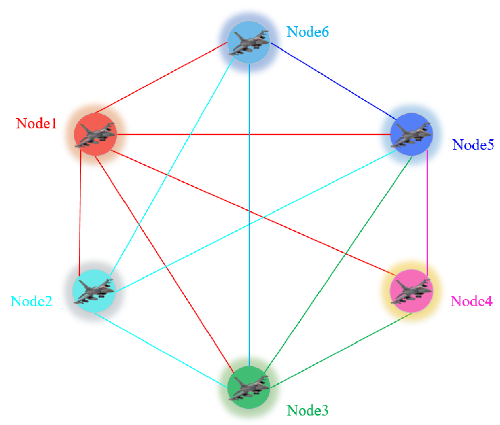
We call each aircraft in the formation as a formation node, assuming that the formation has a total of N nodes, $P_{\mathrm{R}}\{x_i,y_i,z_i\}(i=1,2,\dots ,N)$, which is the actual position of node i; $P_I\{x_{Ii},y_{Ii},z_{Ii}\}(i=1,2,\dots ,N)$, is the position of the INS solution output. The detailed schematic diagram is shown in Figure 1.

Without the aid of an altimeter, the absolute position information of node i and node j can be solved by least squares or Kalman filter method through the following equations:

$$\{\begin{array}{l}{\rho }_i=\sqrt{{(x_{s1}-x_i)}^2+{(y_{s1}-y_i)}^2+{(z_{s1}-z_i)}^2}\\ {\rho }_{INS-i}=\sqrt{{(x_{s1}-x_{Ii})}^2+{(y_{s1}-y_{Ii})}^2+{(z_{s1}-z_{Ii})}^2}\end{array}$$

(1)

$$\{\begin{array}{l}{\rho }_j=\sqrt{{(x_{s2}-x_j)}^2+{(y_{s2}-y_j)}^2+{(z_{s2}-z_j)}^2}\\ {\rho }_{INS-j}=\sqrt{{(x_{s2}-x_{Ij})}^2+{(y_{s2}-y_{Ij})}^2+{(z_{s2}-z_{Ij})}^2}\end{array}$$

(2)

In the same way, with the aid of an altimeter, on the basis of Equations (1) and (2), the absolute position information of node i and node j can be obtained by combining the following equations:

$$\{\begin{array}{l}{\rho }_{Hi}=R_e+H_i\\ {\rho }_{IH-i}=\sqrt{{(x_{Ii}-0)}^2+{(y_{Ii}-0)}^2+{(z_{Ii}-0)}^2}\end{array}$$

(3)

$$\{\begin{array}{l}{\rho }_{Hj}=R_e+H_j\\ {\rho }_{IH-j}=\sqrt{{(x_{Ij}-0)}^2+{(y_{Ij}-0)}^2+{(z_{Ij}-0)}^2}\end{array}$$

(4)

where $R_e$ is the average earth radius; $H_i$ is the elevation reading of node I; and $H_j$ is the elevation reading of node j. Other parameters can be interpreted by referring to Figure 1 or reference [24].

(2)

Relative Navigation Information Construction of Distributed Joint Navigation and Positioning:

The mutual ranging value $D_{ij}^m$ between node i and node j can be expressed as:

$$\begin{array}{ll}{D}_{ij}^m& =\Vert D_j-D_i\Vert \\ & =\sqrt{{(x_j^{}-x_i^{})}^2+{(y_j^{}-y_i^{})}^2+{(z_j-z_i)}^2}+\delta D_{ij}^m\hfill \\ & =D_{ij}^{}+\delta D_{ij}^m\hfill \end{array}$$

(5)

In the formula, $D_{ij}^{}$ is the real relative position among the formation members i and j; $\delta D_{ij}^m$ is the ranging error; and $\delta D_{ij}^m$~$N(0,{\sigma }_{D\_ij}^2)$, ${\sigma }_{D\_ij}^2$ is the ranging variance.

The relative angle between node i and node j measured by the node i angle sensor is

$$\{\begin{array}{l}{\theta }_{m1}={\theta }_1+\mathsf{\Delta }{\theta }_1\\ {\theta }_{m2}={\theta }_2+\mathsf{\Delta }{\theta }_2\end{array}$$

(6)

where ${\theta }_{m1}$ and ${\theta }_{m2}$ are the measured values of the pitch and azimuth of node j relative to node i in the body coordinate system (as shown in Figure 1); ${\theta }_1$ and ${\theta }_2$ represent the real values of the pitch and azimuth, respectively; $\mathsf{\Delta }{\theta }_1$ and $\mathsf{\Delta }{\theta }_2$ represent the angle measurement error of the pitch and azimuth, assuming that they meet the Gaussian white-noise process; that is, $\mathsf{\Delta }{\theta }_1\sim N(0,{\sigma }_{{\theta }_1}^2)$, $\mathsf{\Delta }{\theta }_2\sim N(0,{\sigma }_{\theta 2}^2)$, ${\sigma }_{\theta 1}^2$, ${\sigma }_{\theta 2}^2$ are the corresponding variances.

To correspond to the navigation information, we decompose $D_{ij}^m$ along the three directions of the carrier coordinate system:

$$\{\begin{array}{l}{D}_{ij-x}^m=D_{ij}^m\cos {\theta }_1\sin {\theta }_2\\ D_{ij-y}^m=D_{ij}^m\cos {\theta }_1\cos {\theta }_2\\ D_{ij-z}^m=D_{ij}^m\sin {\theta }_1\end{array}$$

(7)

Assuming that the relative ranging error and angle error are relatively small, according to the infinitesimal equivalent replacement principle, there are

$$\{\begin{array}{l}\cos (\mathsf{\Delta }{\theta }_1)\approx 1\\ \cos (\mathsf{\Delta }{\theta }_2)\approx 1\\ \sin (\mathsf{\Delta }{\theta }_1)\approx {\theta }_1\\ \sin (\mathsf{\Delta }{\theta }_2)\approx {\theta }_2\end{array}$$

(8)

Ignoring higher-order small quantities, we have

$$\{\begin{array}{l}\delta D_{ij}^m\mathsf{\Delta }{\theta }_1\approx 0\\ \delta D_{ij}^m\mathsf{\Delta }{\theta }_2\approx 0\\ \mathsf{\Delta }{\theta }_1\mathsf{\Delta }{\theta }_2\approx 0\end{array}$$

(9)

It can be obtained from Equations (1)~(5)

$$\{\begin{array}{l}{D}_{ij-x}^m=D_{ij-x}-{\kappa }_{x1}\\ D_{ij-y}^m=D_{ij-y}-{\kappa }_{y1}\\ D_{ij-z}^m=D_{ij-z}-{\kappa }_{z1}\end{array}$$

(10)

where, $D_{ij-x}$, $D_{ij-y}$, and $D_{ij-z}$ are the components of the real relative position along the three directions of the body coordinate system; and the specific expressions of ${\kappa }_{x1}$, ${\kappa }_{y1}$, and ${\kappa }_{z1}$ are as follows:

$$\{\begin{array}{l}{\kappa }_{x1}=-\delta D_{ij}^m\cos {\theta }_1\cos {\theta }_2+\mathsf{\Delta }{\theta }_1{D}_{ij}^{}\sin {\theta }_1\sin {\theta }_2-\mathsf{\Delta }{\theta }_2{D}_{ij}^{}\cos {\theta }_1\cos {\theta }_2\\ {\kappa }_{y1}=-\delta D_{ij}^m\cos {\theta }_1\cos {\theta }_2+\mathsf{\Delta }{\theta }_1{D}_{ij}^{}\sin {\theta }_1\cos {\theta }_2+\mathsf{\Delta }{\theta }_2{D}_{ij}^{}\cos {\theta }_1\sin {\theta }_2\\ {\kappa }_{z1}=-\delta D_{ij}^m\sin {\theta }_1-\mathsf{\Delta }{\theta }_1{D}_{ij}^{}\cos {\theta }_1\end{array}$$

(11)

Similarly, omitting the redundant derivation process, we can obtain the relative velocity relationship between node i and node j as follows:

$$\{\begin{array}{l}{V}_{ij-x}^m=V_{ij-x}-{\mu }_{x1}\\ V_{ij-y}^m=V_{ij-y}-{\mu }_{y1}\\ V_{ij-z}^m=V_{ij-z}-{\mu }_{z1}\end{array}$$

(12)

$$\{\begin{array}{l}{\mu }_{x1}=-\delta V_{ij}^m\cos {\varphi }_1\cos {\varphi }_2+\mathsf{\Delta }{\varphi }_1{V}_{ij}\sin {\varphi }_1\sin {\varphi }_2-\mathsf{\Delta }{\varphi }_2{V}_{ij}\cos {\varphi }_1\cos {\varphi }_2\\ {\mu }_{y1}=-\delta V_{ij}^m\cos {\varphi }_1\cos {\varphi }_2+\mathsf{\Delta }{\varphi }_1{V}_{ij}\sin {\varphi }_1\cos {\varphi }_2+\mathsf{\Delta }{\varphi }_2{V}_{ij}\cos {\varphi }_1\sin {\varphi }_2\\ {\mu }_{z1}=-\delta V_{ij}^m\sin {\varphi }_1-\mathsf{\Delta }{\varphi }_1{V}_{ij}\cos {\varphi }_1\end{array}$$

(13)

where ${\varphi }_1$ and ${\varphi }_2$ have similar meanings to ${\theta }_1$ and ${\theta }_2$; and other parameters $\delta V_{ij}^m$, $V_{ij-x}$, $V_{ij-y}$, and $V_{ij-z}$ are also similar and are not repeated here.

Thus far, the relative position information and relative velocity information have been constructed, and they are the state variables for the subsequent construction of joint navigation and positioning measurement equations.

2.3. Platform Composition and Overall Architecture of Distributed Joint Navigation and Positioning System

We assume that the joint positioning system of each node consists of a set of airborne data links, INS and ranging/velocity sensors, and a networking computer. In the joint positioning process, the local geographic coordinate system is selected as the navigation system, and the directions of the three axes are north, east, and down, respectively. The LEO and INS data of this node are transmitted to the airborne data link, and the transmitted LEO and INS data include position information and velocity information as well as the status word and frame number; the airborne data link has the functions of real-time ranging and communication; thus, we used laser rangefinders to measure the position $D_{ij}^m$$(i=1,2,\dots ,n,i\ne j)$ between each node in the formation, and at the same time, communicate the joint navigation ranging and velocity measurement information to each other in real time through radio communication equipment. Finally, the ranging information of all nodes is transmitted to the networking computer for joint positioning calculation. The node joint positioning system framework is shown in Figure 2.

As one of the core devices of the system, the airborne data link is a link device based on data link technology, which can form point-to-point, point-to-multipoint data links and mesh data links and generally has real-time ranging and communication functions [25]; a distributed non-central mesh data link structure is shown in Figure 3.

2.4. Ranging and Time Synchronization of Distributed Joint Navigation and Positioning

2.4.1. Ranging Scheme

After the formation aircraft assemble in the designated airspace, according to the time system of each aircraft, the data link of the fleet is powered on and starts ranging at a specified time. There are three commonly used radio ranging methods: one-way ranging method, double-side two-way ranging method, and dual one-way ranging method. The one-way ranging method requires expensive high-precision crystal oscillators [26], and the double-side two-way ranging equipment is complicated, and it is difficult to measure the distance of multiple machines at the same time. Therefore, the co-positioning system adopts the t dual one-way ranging method [27]. The principle is as follows:

The data link device (hereinafter referred to as device i) equipped with node i transmits one-way ranging signals and simultaneously receives one-way ranging signals from other devices. Taking the mutual ranging between devices i and j as an example, let $\mathsf{\Delta }{\tau }_{ij}$ be the time synchronization error between the clocks of devices i and j; $t_{ij}$ is the radio signal propagation time between devices i and j (usually on the microsecond scale [28]); $t_1$ is the signal propagation time measured by device i; and $t_2$ is the signal propagation time measured by device j. Then,

$$t_1=t_{ij}+\mathsf{\Delta }{\tau }_{ij}$$

(14)

$$t_2=t_{ij}-\mathsf{\Delta }{\tau }_{ij}$$

(15)

During the ranging process, the working mechanisms of devices i and j are exactly the same. Taking device i as an example: device i measures $t_1$, and at the same time, the receiving device j transmits $t_2$; then, it can be calculated from Equations (14) and (15):

$$t_{ij}=\frac{(t_1+t_2)}{2}$$

(16)

$$\mathsf{\Delta }{\tau }_{ij}=\frac{(t_1-t_2)}{2}$$

(17)

The ranging values for devices i and j are

$$D_{ij}^m=c\times t_{ij}$$

(18)

where c is the velocity of light.

It can be seen that the dual one-way ranging method can calculate the position between nodes, and at the same time, it can also calculate the time synchronization error between the clocks (ns magnitude [29]) of the airborne data link equipment, which is conducive to the simultaneous ranging of multiple machines.

2.4.2. Time Synchronization

There are the following three time synchronization problems in the joint positioning process of formation node networking:

(1)

Time synchronization between the onboard data link clocks of each node:

To achieve synchronous mutual ranging, the airborne data link should have a unified time scale, but each airborne data link cannot achieve precise time synchronization when they are turned on, so there is a time bias between their time scales. In the dual one-way ranging method, the time bias between the clocks can be calculated according to Equation (17). With the clock of an airborne data link device as a reference, time synchronization can be achieved by adjusting the clocks of all devices.

(2)

Time synchronization between the INS of node i and the airborne data link device:

Since the synchronous ranging moment of the airborne data link i is not necessarily the measurement moment of the INS-i, there is a time bias $\mathsf{\Delta }{t}_i$ between the airborne data link device i and the INS-i. $\mathsf{\Delta }{t}_i$ is a random constant. If the INS has 100 Hz output, assuming that the aircraft velocity is 340 m/s, then the position error caused by $\mathsf{\Delta }{t}_i$ within ±1 ms is usually within ±5 m, and this value is negligibly relative to the position error of INS. Therefore, in the process of joint positioning calculation, it can be considered that the clocks between the airborne data link and each INS are completely synchronized.

(3)

Time synchronization between nodes (including INS) and satellites:

As mentioned in Section 2.1, since we use the LEO constellation as the navigation framework, and the essence of the LEO satellites is communication satellite, the clock bias between the LEO constellation and the user terminal can be eliminated in a way similar to full duplex. When solving the absolute position and relative position of the user terminal, we can eliminate the time synchronization error by means of the “duplex” system, and we will not consider the variable of clock biases.

3. Establishment of Distributed Joint Navigation and Positioning Model

3.1. State Model

Without loss of generality, we only take the two formation nodes, Node 1 and Node 2, as the study objects; select the position error and velocity error as state variables; supplement the Markov noises of gyroscope and accelerometer as state variables; and establish the following system state equation [30]:

$${\dot{X}}_{JP}=\mathsf{\Gamma }{X}_{JP}+\mathsf{\Phi }{W}_{JP}$$

(19)

$$\begin{gathered} X_{JP}=[\begin{array}{ccccccccc}{\phi }_N& {\phi }_E& {\phi }_D& \delta V_N& \delta V_E& \delta V_D& \delta \lambda & \delta L& \delta h\end{array} \\ \begin{array}{cccccc}{\xi }_{gx}& {\xi }_{gy}& {\xi }_{gz}& {\xi }_{ax}& {\xi }_{ay}& {\xi }_{az}\end{array}{]}^{\mathrm{T}} \end{gathered}$$

(20)

where $\phi =[\begin{array}{ccc}{\phi }_N& {\phi }_E& {\phi }_D\end{array}]$ is the misalignment angle of the platform between the platform coordinate system and the navigation coordinate system in the N, E, and D directions; $\delta V={\left[\begin{array}{cc}\delta V_N& \begin{array}{cc}\delta V_E& \delta V_D\end{array}\end{array}\right]}^{\mathrm{T}}$ is the three-dimensional velocity error; $\delta P=\left[\begin{array}{ccc}\delta \lambda & \delta L& \delta h\end{array}\right]$ is the three-dimensional position error, and ${\xi }_g=\left[\begin{array}{ccc}{\xi }_{gx}& {\xi }_{gy}& {\xi }_{gz}\end{array}\right]$ is the first-order Markov drift of the gyroscope; ${\xi }_a=\left[\begin{array}{ccc}{\xi }_{ax}& {\xi }_{ay}& {\xi }_{az}\end{array}\right]$ is the first-order Markov drift of the accelerometer. $\mathsf{\Gamma }$ is a 15 × 15-dimensional matrix, $X_{JP}$ is an 15 × 1-dimensional matrix, $\mathsf{\Phi }$ is a 15 × 6-dimensional matrix, and $W_{JP}$ is a 6 × 1-dimensional matrix [31,32].

3.2. Measurement Model

Here, we assume that the relative position information and relative velocity information (which can be obtained by angle measurement and distance measurement) can be measured between the aircraft, and the relative position and relative velocity measured by the distance measurement and velocity measurement sensors are converted from the body coordinate system to the navigation coordinate system by

$$D_{12}^n=C_b^n(D_{12}^b+\delta D_{12}^b)$$

(21)

$$V_{12}^n=C_b^n(V_{12}^b+\delta V_{12}^b)$$

(22)

where $\delta D_{12}^b$ and $\delta V_{12}^b$ are distance measurement and velocity measurement errors, assuming that they are all Gaussian white noise with mean zero and variance ${\sigma }_{Db\_12}^2$ and ${\sigma }_{Vb\_12}^2$, respectively; $C_b^n$ is the transformation matrix from the carrier coordinate system to the navigation coordinate system, and its expression is as follows [33]:

$$C_b^n=\left[\begin{array}{ccc}\cos \alpha \cos \beta & -\cos \gamma \sin \beta +\sin \gamma \cos \beta \sin \alpha & \sin \gamma \sin \beta +\cos \gamma \cos \beta \sin \alpha \\ \cos \alpha \sin \beta & \cos \gamma \sin \beta +\sin \gamma \sin \beta \sin \alpha & \sin \gamma \cos \beta +\cos \gamma \sin \beta \sin \alpha \\ -\sin \alpha & \cos \alpha \sin \gamma & \cos \alpha \cos \gamma \end{array}\right]$$

(23)

where $\alpha$, $\beta$, and $\gamma$ represent the pitch, yaw, and roll of Node 1; $D_{12}$ and $V_{12}$ are the relative position and relative velocity between Node 1 and Node 2, and the relationship is as follows:

$$D_1^n-D_2^n=D_{12}^n$$

(24)

$$V_1^n-V_2^n=V_{12}^n$$

(25)

Since a high-precision navigation solution can be obtained between Node 1 and Node 2 by means of pseudorange-pseudorange rate [24], it can be considered that the navigation solution is approximately equal to their real values. Then, transmit their position and velocity solutions to each other by means of inter-node communication. At the same time, we assume that Node 1 and Node 2 are equipped with an inertial measurement unit (IMU) with a good index so that the accumulated error of the measurement is relatively slow; therefore, it can be considered ${\tilde{C}}_b^n\approx C_b^n$. Taking Node 1 as an example, the relationship between the relative navigation information, that is, the position and velocity deviation between the nodes, can be written as follows:

$$\begin{array}{ll}{\stackrel{⌢}{D}}_1^n& -{\tilde{D}}_2^n-D_{12}^n\\ & =M_e^n({\stackrel{⌢}{D}}_1^e-{\tilde{D}}_2^e)-{\tilde{C}}_e^n(D_{12}^b+\delta D_{12}^b)\\ & =M_e^n({\stackrel{⌢}{D}}_1^e-{\stackrel{⌢}{D}}_2^e-\delta D_2)-{\tilde{C}}_e^n(D_{12}^b+\delta D_{12}^b)\end{array}$$

(26)

$$\begin{array}{ll}{\stackrel{⌢}{V}}_1^n& -{\tilde{V}}_2^n-V_{12}^n\\ & ={\stackrel{⌢}{V}}_1^n-{\tilde{V}}_2^n-{\tilde{C}}_b^n(V_{12}^b+\delta V_{12}^b)\\ & ={\stackrel{⌢}{V}}_1^n-V_2^n-\delta V_2-{\tilde{C}}_b^n(V_{12}^b+\delta V_{12}^b)\end{array}$$

(27)

where ${\stackrel{⌢}{D}}_1^n$ and ${\stackrel{⌢}{V}}_1^n$ are the position and velocity parameters of Node 1 in the Earth-centered Earth-fixed (ECEF) coordinate system, and ${\tilde{D}}_2^n$ is the position parameter to be corrected of Node 2; in the case of a short baseline, the influence of the Earth’s curve radian can be ignored, and it can be approximated by

$$D_{12}^b=C_b^n{M}_e^n(D_1^e-D_2^e)$$

(28)

where $M_e^n$ is the transformation matrix of longitude-latitude-high to north-east-down; if the radius of curvature of the coordinate system where Node 1 and Node 2 are located is $R_{Mer}$, the radius of curvature of the Prime Vertical is $R_{\mathrm{Pr}i}$, the latitude is L, and the height is h. Then, the form of $M_e^n$ is as follows [34]:

$$M_e^n=\left[\begin{array}{ccc}{R}_{Mer}+h& & \\ & (R_{\mathrm{Pr}i}+h)\cos L& \\ & & -1\end{array}\right]$$

(29)

According to Formulas (26) and (27), $Z_D={\stackrel{⌢}{D}}_1^n-{\tilde{D}}_2^n-D_{12}^n$ and $V_D={\stackrel{⌢}{V}}_1^n-{\tilde{V}}_2^n-V_{12}^n$ are selected as the observed variables, and the Kalman filter observation equation is constructed as follows:

$$\{\begin{array}{c}{Z}_D=H_D{X}_{JP}+{\sigma }_D\\ Z_V=H_V{X}_{JP}+{\sigma }_V\end{array}$$

(30)

where the specific expressions of $H_D$ and $H_V$ are as

$$\{\begin{array}{c}{H}_D=\left[\begin{array}{ccc}{O}_{3\times 3}& -I_{3\times 3}& \begin{array}{ccc}{O}_{3\times 3}& O_{3\times 3}& O_{3\times 3}\end{array}\end{array}\right]\\ H_V=\left[\begin{array}{ccc}{O}_{3\times 3}& O_{3\times 3}& \begin{array}{ccc}-M_e^n& O_{3\times 3}& O_{3\times 3}\end{array}\end{array}\right]\end{array}$$

(31)

where ${\sigma }_D$ and ${\sigma }_V$ are the ranging and velocity noise after coupling ${\sigma }_{Db\_12}$ and ${\sigma }_{Vb\_12}$, which we model as multiplicative noise with the modulo length of the position and velocity vectors.

4. Simulation Verification

4.1. Simulation Parameter Configuration

We take two distributed nodes as an example: the initial baseline interval between them is 10 km, and the height is also 10 km. The reference formation aircraft is located in the airspace assembly trajectory shown in Figure 4, the flight velocity is 200 m/s, the corresponding sensor data are generated to verify the effectiveness of the established collaborative navigation algorithm. The reference aircraft, LEO constellation, and IMU indicators are shown in

Table 1. Reference aircraft and navigation sensor parameters.

Parameter	Node 1	Node 2
Gyroscope random walk ($deg/\sqrt{h}$)	0.0005	0.0005
Accelerometer random walk ($m/s/\sqrt{h}$)	0.003	0.003
Gyroscope first-order Markov noise RMS ($deg/\sqrt{h}$)	0.002	0.002
Accelerometer first-order Markov noise RMS ($\mu g_0$)	10	10
Position noise (m)	0.1	0.1
Velocity noise (m/s)	0.01	0.01
Data link ranging error (m)	10	10
Flight velocity (m/s)	200	200
Flight duration (s)	420	420

and

Table 2. LEO constellation parameters.

Parameter	Value
Constellation configuration type	Walker [36]
Track height (km)	1250
Orbital inclination (deg)	99
Number of orbital faces	20
Number of satellites per orbit (total/orbit)	50
Number of satellites per orbit	1000

. Since the Walker constellation has the same orbital height and uniformly distributed inclined orbital plane, it is a very suitable design scheme for the LEO constellation, and most broadband LEO constellations are deployed with this design scheme [35]. Secondly, considering the coverage characteristics in challenging environments, we deliberately set the orbital inclination to a high orbital inclination (99 deg, see Table 2) to cover the high latitudes of the Earth and the north and south poles.

4.2. Simulation Results

According to the parameter settings in Section 4.1, we divide the algorithm into two scenarios. The first is a joint navigation and positioning scenario without an altimeter assistance, and the other is a joint navigation and positioning scenario assisted by an altimeter. Then, the two scenarios are simulated and analyzed separately. Here, we only take Node 1 and Node 2 as examples for simulation, where NPE and NVE and |alt, O represent north position error, north velocity error, altimeter error (symbol “|” means under the condition that the altimeter error is x m), and original trajectory, respectively. The meaning of other parameters refers to these expressions.

4.2.1. Joint Navigation and Positioning Scenarios without an Altimeter Assistance

In the absence of an altimeter assistance, the simulation results are shown in Figure 5, in which we compare and verify the INS individual navigation and positioning results corresponding to Node 1 and Node 2 to verify the convergence effect of the algorithm.

From Figure 5, we can see that in the scenario without an altimeter assistance, the position error of Node 1 and Node 2 does not fluctuate too much, and both converge to zero, and as the velocity error is also very small, it also shows a convergence trend. For the INS autonomous joint navigation scheme, we found that the pure INS autonomous joint navigation error diverges faster, and the error is relatively large. The above results are also fully reflected on the final 3D trajectory and projected trajectory error curves, and the results are consistent; this result can be seen in Figure 5c,d. It can be clearly seen from Figure 5 that the navigation and positioning results of the INS are significantly larger than the navigation and positioning results of the corresponding nodes. These results fully show that the joint navigation and positioning algorithm without an altimeter can effectively suppress the divergence of pure INS navigation and positioning. To facilitate quantitative analysis,

Table 3. Statistics of pure INS navigation positioning position error.

Indicators	Node 1			Node 2
	N	E	D	N	E	D
Mean (m)	−130.71	97.47	−91.31	−147.07	−154.98	−91.26
STD (m)	119.91	87.73	86.10	124.78	119.79	86.05

,

Table 4. Statistics of joint navigation and positioning position error without an altimeter.

Indicators	Node 1			Node 2
	N	E	D	N	E	D
Mean (m)	−3.23	6.50	−13.8	−8.30	5.11	−16.98
STD (m)	6.80	5.89	14.11	5.02	7.55	11.79

,

Table 5. Statistics of pure INS navigation position positioning velocity error.

Indicators	Node 1			Node 2
	N	E	D	N	E	D
Mean (m/s)	−1.02	0.51	−0.69	−1.03	0.49	−0.69
STD (m/s)	0.63	0.43	0.45	0.63	0.41	0.45

and

Table 6. Statistics of joint navigation positioning velocity error without an altimeter.

Indicators	Node 1			Node 2
	N	E	D	N	E	D
Mean (m/s)	0.01	0.04	−0.01	−0.02	−0.09	−0.06
STD (m/s)	0.22	0.19	0.20	0.21	0.39	0.37

shows the corresponding statistical results of indicators.

As can be seen from the statistical results in Table 3, Table 4, Table 5 and Table 6:

(1)

For the position error curve, the position errors of Node 1 and Node 2 in the north (N), east (E), and down (D) directions are not very different, and the mean error is in the order of 1 m in both the N and E directions, while the error in the D direction is relatively large, reaching the order of 10 m, mainly because the GNSS elevation accuracy makes it difficult to distinguish the height of the moving node [32], which results in a larger error compared to the N and E directions. Correspondingly, the position error accuracy (STD) of two nodes has a similar behavior. In addition, the mean value of the pure INS autonomous navigation error of the two nodes is basically greater than 100 m, and the accuracy is also higher than 100 m. It can be seen that even without the aid of an altimeter, the algorithm can significantly suppress the problem of pure INS position divergence.

(2)

For the velocity error curve, the velocity errors of Node 1 and Node 2 in the N, E, and D directions are also not much different. The accuracy is in the order of 0.1 m/s; in comparison, the mean of the respective pure INS navigation errors of the two nodes is about 1 m/s, and the accuracy is also close to 1 m/s. Similarly, the algorithm can also obviously suppress the problem of pure INS navigation velocity divergence.

It can be seen from the above analysis that without the aid of an altimeter, the joint navigation and positioning algorithm can significantly suppress the divergence of the pure INS and greatly improve the accuracy of navigation and positioning, meeting the needs of most joint navigation and positioning services.

4.2.2. Altimeter-Assisted Joint Navigation and Positioning Scenarios

In the added altimeter scenario, we set the auxiliary altimeter error to 0 m (no error), 10 m, and 30 m for the simulations, and the results are shown in Figure 6. In addition, as a comparison, we simulated without an altimeter auxiliary scene together, and the results are also added as a comparative analysis, where alt = x m means that the altimeter error is x m (x = 0, 10, 30).

It can be seen from the simulation results in Figure 6 that the addition of an altimeter, especially the use of an unbiased altimeter, can further improve the performance of joint navigation and positioning; in particular, the improvement effect in the D direction is the best. In addition, we can also see that, as the altimeter error gradually increases from 0 m, 10 m, to 30 m, the corresponding joint navigation positioning error also gradually increases; the final convergence result depends on the fixed altimeter bias we used, and it is expected that the larger the fixed altimeter bias, the larger the final convergence result. In addition, it can be observed that with the help of the altimeter, the relative elevation information of the moving nodes can be measured, significantly improving the accuracy of the joint positioning system in the elevation direction. Similarly, the improvement of elevation also depends on the error accuracy of the altimeter used: the higher the accuracy of the altimeter, the more obvious the improvement effect. To carry out quantitative analysis, we also obtained statistics on the corresponding statistical indicators, and the specific error statistics are shown in

Table 7. Statistics of joint navigation and positioning position error in the altimeter presence scenario.

Node	Alt (m)	Mean (m)			STD (m)
		N	E	D	N	E	D
	0	−1.45	3.49	−0.41	5.73	7.22	0.64
Node 1	10	−1.74	10.58	9.37	8.59	11.83	1.15
	30	−2.33	24.78	28.96	15.56	24.37	2.98
	0	−4.54	−4.39	−0.39	15.54	19.47	0.76
Node 2	10	−3.46	0.32	9.40	16.11	21.08	1.23
	30	−1.29	9.75	28.99	16.17	27.90	3.02

and

Table 8. Statistics of joint navigation positioning velocity error in the altimeter presence scenario.

Node	Alt (m)	Mean (m/s)			STD (m/s)
		N	E	D	N	E	D
	0	−0.008	−0.42	−0.01	0.11	0.21	0.03
Node 1	10	−0.11	−0.53	−0.01	0.11	0.22	0.03
	30	−0.16	−0.59	−0.02	0.16	0.24	0.02
	0	−0.09	−1.05	−0.02	0.28	0.45	0.03
Node 2	10	−0.10	−1.00	−0.02	0.29	0.45	0.04
	30	−0.12	−0.91	−0.02	0.30	0.46	0.04

.

From the statistics results of Table 7 and Table 8, it can be seen that the addition of an altimeter can significantly improve the accuracy of joint navigation and positioning.

(1)

For the position error curve, with the assistance of an unbiased altimeter, the mean errors of Node 1 and Node 2 in the N and E directions are also in the order of 1 m, and compared with the altimeter-free scene, the error was significantly improved, especially in the D direction, which has an error of the order of 0.1 m showing relative improvement of two orders of magnitude. For accuracy, the N and E directions were also significantly improved, and the D direction accuracy also improved by two orders of magnitude. When the altimeter deviation is 10 m and 30 m, the mean values of the position errors of Node 1 and Node 2 in the N, E, and D directions also gradually increase, and the accuracy also gradually deteriorates. However, we deduct the fixed error accuracy, and it can be found that the corresponding position accuracy is also very impressive.

(2)

For the velocity error curve, compared with the scene without altitude assistance, although the addition of the altimeter does not significantly improve the velocity error in the N and E directions, the velocity error improvement in the D direction is very significant. The accuracy is improved by one order of magnitude. In addition, as the altimeter deviation increases, the corresponding joint navigation and positioning velocity indicators also gradually deteriorate. Similarly, when we deduct the fixed deviation, we can also obtain a good joint navigation and positioning effect, which is also in line with expectations.

We can see from the above analysis results that the addition of an altimeter can significantly improve the performance of joint navigation and positioning, especially in the D direction. Thus, it can be seen that the algorithm effect can be further improved by combining an altimeter, which can meet the vast majority of joint location service requirements in challenging environments.

4.2.3. Influence of Formation Baseline on Joint Navigation and Positioning Performance

To explore the impact of different formation node baseline intervals on joint navigation and positioning performance, in this subsection, we study the effect of joint navigation and positioning of nodes at different baseline intervals. To this end, we set the formation node baseline interval as 10 m, 100 m, 500 m, 1 km, 5 km, and 10 km and then use an unbiased altimeter to conduct auxiliary navigation analysis. The simulation results are shown in Figure 7, where B represents the baseline interval.

It can be seen from the simulation results in Figure 7 that with the increase of baseline interval, the fluctuation of joint navigation positioning position error and velocity error also increases gradually, but overall:

(1)

For the N direction error: regardless of Node 1 or Node 2, the position error finally converges between 0 m~10 m, the maximum fluctuation is about 50 m, the velocity error almost converges to zero, and the maximum fluctuation is not more than 1 m/s;

(2)

For the E direction error: the position error finally converges between 0 m and 20 m, and the maximum fluctuation is about 50 m. For the velocity error, the error of node 1 and Node 2 increases with the increase of the baseline interval, and the final convergence error also increased, respectively, but ultimately did not exceed 1 m/s, and the maximum fluctuation did not exceed 2 m/s;

(3)

For the D direction error: whether it is the position error or the velocity error, the final result converges to zero, and the maximum fluctuation is less than 3 m and 0.2 m/s, respectively.

For different baseline interval errors, we can select the appropriate formation flight application according to the size range of the error, specifically:

(1)

When the baseline interval is between 10 m and 1 km, the error is relatively small, which is very suitable for small UAVs formation flying situation;

(2)

When the baseline interval increases to more than 1 km, at this time, the error is relatively large, but the final error curves all have zero-crossing points, which means that the error is convergent, and this situation is suitable for the formation of large- and medium-sized UAVs.

The above analysis results show that our proposed algorithm is suitable even for relatively large baseline intervals, the maximum joint navigation positioning position error fluctuation does not exceed 50 m, and the maximum velocity error fluctuation does not exceed 2 m/s, which is sufficiently accurate for most joint navigation and positioning requirements.

5. Algorithm Comparison

In this section, to compare the universality, effectiveness, superiority, and potential superiority of the algorithm horizontally and vertically, we start from three perspectives, that is, using the current LEO constellations with relatively complete deployments, such as SpaceX, OneWeb, and Telesat, to compare and verify the universality and effectiveness of the algorithm horizontally. The vertical comparison between the proposed algorithm and the current four GNSS navigation systems is carried out to verify the superiority of the algorithm. Furthermore, our proposed algorithm is compared with existing advanced algorithms to verify the advantages and potential superiority of our algorithm.

5.1. Comparison of Different LEO Systems

As a horizontal comparison, we use an unbiased altimeter for assistance. The simulation results are shown in Figure 8 where, as a reference, we use the self-designed algorithm as a comparison to simulate together. The specific parameters of the three constellations SpaceX, OneWeb, and Telesat can be found in reference [37].

It can be found from the simulation results in Figure 8 that, on the whole, the three systems give good joint navigation and positioning results although the errors of each system in individual directions may have some fluctuations, which mainly depends on the orbital parameters of each constellation, such as the satellite orbit height, inclination, the distribution of satellites, and the number of satellites in each orbit. However, the final position error and velocity error of each LEO system are convergent, which means that the algorithm we propose is universal, suitable for present most LEO constellations, and can be used as a reference scheme for joint navigation and positioning existing LEO systems and especially as a reference for future integrated communication, navigation (ICN) technology navigation, and positioning technology plans.

5.2. Comparison with MEO Constellation Algorithm

As a vertical comparison, we also used an unbiased altimeter for assistance, and the simulation results are shown in Figure 9. Similarly, as a reference, we simulated the self-designed algorithms as a comparison. The specific parameters of the four major MEO systems BDS, GPS, Galileo, and GLONSS can be found in reference [38].

Compared with the simulation results of Figure 9, our proposed algorithm has greater accuracy advantages in both the position error and the velocity error than the traditional MEO constellation system, especially in the N and E directions. In addition, similar conclusions can be drawn on the final trajectory error curve. This shows that for the future ICN navigation and positioning scheme, MEO-based constellations are not a well-fitting alternative because the main reason for the larger navigation and positioning error of the MEO constellation is that the satellite orbit height is higher than the LEO constellation at the same observation time; as a result, GNSS signal propagation experiences more paths than LEO constellation, and it suffers more serious interference. In addition, if the orbit height is too high, the loss of GNSS signal power will be greater, and the propagation delay will also increase. Therefore, the LEO constellation can be regarded as a considerable option for future ICN technology.

5.3. Comparison with Other Algorithms

To verify the superiority and potential superiority of our proposed algorithm, we compare it with the existing advanced navigation and positioning algorithms. Here, we only take the indicators of Node 1 as an example for comparison. The detailed comparison indicators is shown in Figure 10 and Figure 11. In addition, we transformed the ENU coordinate system and the NED coordinate system correspondingly; among them, N/A means that no specific data are given in the original papers.

From the statistical histogram of position error in Figure 10, our proposed algorithm has certain advantages in terms of mean over algorithm [40] and algorithm [24]; in terms of accuracy, our algorithm is comparable to algorithm [40], but the algorithm [40] fluctuates greatly in the D direction, and our algorithm is just the opposite. In addition, our algorithm also has certain advantages compared with the algorithm [39] and the algorithm [24], and especially compared with the algorithm [39], the accuracy is improved by one order of magnitude.

From the velocity error statistical histogram in Figure 11, the algorithm we propose has a great advantage over the algorithm [40] in terms of mean, and the performance is improved by one order of magnitude; compared with algorithm [24], although the standard deviation of the algorithm [24] is relatively good in the D direction, our proposed algorithm also has certain advantages in the mean and standard deviation, especially in the N direction. From the point of view of accuracy, our proposed algorithm has great advantages compared with algorithm [41], especially in the D direction, as the performance is improved by 95.38%. Compared with algorithm [40] and algorithm [24], the performance is roughly the same, but the mean error of our algorithm is smaller, which means that the error fluctuation is smaller, and the algorithm is relatively more stable.

From the above comparison results, our algorithm has certain advantages or potential advantages compared with some advanced transposition positioning algorithms [24,39,40,41]. For localization performance, in terms of mean and standard deviation, our algorithm is simple in integration and easy to implement in engineering, thereby reducing the corresponding practical application cost. More importantly, our algorithm is oriented to future ICN technology, so it has potentially important application value.

6. Conclusions

In this paper, we take the distributed joint navigation between formation aircraft as the research background and propose a bidirectional distributed joint correction navigation and positioning model that uses relative position information and velocity information to correct the navigation state among formation members. Through the set LEO constellation, the experimental scenario is divided into two scenarios without an altimeter assistance and with an altimeter assistance, with the simulation experiment verifying the effectiveness of the model in a challenging environment. Then, the two scenarios are compared and analyzed, and from the horizontal comparison of the existing main LEO constellations, the universality and effectiveness of the algorithm are strictly verified, and the MEO constellations are compared vertically to verify the superiority of the algorithm. Finally, compared with the existing advanced navigation and positioning algorithms, the superiority and potential superiority of the algorithm are verified.

The experiments show the following:

(1)

Compared with the traditional leader-fellow collaborative navigation structure that relies on the leader node, our scheme is a distributed collaborative navigation and positioning scheme, which, without the distinction between leader and follower, is a flexible formation collaboration scheme; when performing special tasks, it will gain huge formation reconfiguration advantages;

(2)

Even without the aid of an altimeter, our algorithm can well suppress the divergence of the pure INS collaborative navigation scheme. With the aid of an altimeter, the collaborative navigation performance is further improved since the altimeter has the advantage of low cost compared with other expensive sensors; thus, it has great practical value;

(3)

Even if the node baseline interval gradually increases, our algorithm position can converge to zero with or without altimeter assistance, which has a certain robustness and can meet the needs of joint navigation and positioning location services in challenging environments. It is suitable for formation flying and other application scenarios that have high requirements for the accuracy and robustness of moving target cooperative navigation.

In addition, due to our use of a wideband LEO constellation design, with some inherent advantages of the LEO constellation, the accuracy and performance of the algorithm can be further improved compared with the MEO constellation navigation algorithm and some existing advanced schemes. Therefore, our algorithm can be regarded as an ICN reference scheme for future joint navigation and positioning, and the research results can provide reference value for the application of basic joint navigation technology and the application in practical engineering.

Of course, with the increase of the baseline interval, our joint navigation and positioning accuracy is not high enough, and the velocity cannot fully converge in individual directions. At the same time, the clock bias elimination technology in this paper needs to be verified through specific engineering experiments. Finally, it is necessary to further study the basic theory of joint navigation and positioning technology, which can provide theoretical support for solving the above problems.

References

1. Barnes, D. GPS status and modernization. In Proceedings of the Munich Satellite Navigation Summit, Alte Kongresshalle, Munich, Germany, 25–27 March 2019; Air Force Space Command: Los Angeles, CA, USA, 2019. [Google Scholar]
2. China Satellite Navigation Office. Development of the BeiDou Navigation Satellite System (Version 4.0); CSNO: Beijing, China, 2019. [Google Scholar]
3. Benedicto, J. Directions 2020: Galileo moves ahead. GPS World, 14 December 2019. [Google Scholar]
4. Langley, R.B. Innovation: GLONASS—Past, present and future. GPS World, 1 November 2017. [Google Scholar]
5. Scherer, J.; Rinner, B. Persistent multi-UAV surveillance with energy and communication constraints. In Proceedings of the IEEE International Conference on Automation Science & Engineering, Fort Worth, TX, USA, 17 November 2016; pp. 1225–1230. [Google Scholar]
6. Minetto, A.; Dovis, F. On the Information Carried by Correlated Collaborative Ranging Measurements for Hybrid Positioning. IEEE Trans. Veh. Technol. 2020, 69, 1419–1427. [Google Scholar] [CrossRef]
7. Guha, M. Technical ecstasy: Network-centric warfare redux. Secur. Dialogue 2021, 1–17. [Google Scholar] [CrossRef]
8. Causa, F.; Vetrella, A.R.; Fasano, G.; Accardo, D. Multi-UAV formation geometries for cooperative navigation in GNSS-challenging environments. In Proceedings of the IEEE/ION Position, Location & Navigation Symposium, Monterey, CA, USA, 7 June 2018; pp. 775–785. [Google Scholar]
9. Yan, Z.; Wang, L.; Wang, T.; Yang, Z.; Chen, T.; Xu, J. Polar Cooperative Navigation Algorithm for Multi-Unmanned Underwater Vehicles Considering Communication Delays. Sensors 2018, 18, 1044. [Google Scholar] [CrossRef] [PubMed] [Green Version]
10. Jin, H.; Yang, T.; Wang, X.; Zhou, G.; Yao, W. Application of multi-sensor information fusion in UAV relative navigation method. J. Natl. Univ. Def. Technol. 2017, 39, 90–95. [Google Scholar]
11. Groves, P.D.; Adjrad, M.; Gao, H.; Ellul, C.D. Intelligent GNSS Positioning using 3D Mapping and Context Detection for Better Accuracy in Dense Urban Environments. In Proceedings of the International Navigation Conference, Glasgow, UK, 8–10 November 2016; Available online: https://discovery.ucl.ac.uk/id/eprint/1524033 (accessed on 3 April 2022).
12. Zhang, G.; Wen, W.; Hsu, L.T. Rectification of GNSS-based collaborative positioning using 3D building models in urban areas. GPS Solut. 2019, 23, 1–12. [Google Scholar] [CrossRef]
13. Hu, J.; Xie, L.; Lum, K.Y.; Xu, J. Multiagent Information Fusion and Cooperative Control in Target Search. IEEE Trans. Control Syst. Technol. 2013, 21, 1223–1235. [Google Scholar] [CrossRef]
14. Zhu, Q.; Zhou, R.; Zhang, J. Connectivity Maintenance Based on Multiple Relay UAVs Selection Scheme in Cooperative Surveillance. Appl. Sci. 2017, 7, 8. [Google Scholar] [CrossRef] [Green Version]
15. Wang, Y.; Chen, X.; Ran, D.; Zhao, Y.; Chen, Y.; Bai, Y. Spacecraft formation reconfiguration with multi-obstacle avoidance under navigation and control uncertainties using adaptive artificial potential function method. Astrodyn 2020, 4, 41–56. [Google Scholar] [CrossRef]
16. Go, O.; Fuyuto, T.; Naoko, O.; Yuya, M.; Kent, Y.; Yuto, T.; Takanao, S.; Yuichi, T. Design and flight results of GNC systems in Hayabusa2 descent operations. Astrodyn 2020, 4, 105–117. [Google Scholar] [CrossRef]
17. Ogawa, N.; Terui, F.; Mimasu, Y.; Yoshikawa, K.; Ono, G.; Yasuda, S.; Tsuda, Y. Image-based autonomous navigation of Hayabusa2 using artificial landmarks: The design and brief in-flight results of the first landing on asteroid Ryugu. Astrodyn 2020, 4, 89–103. [Google Scholar] [CrossRef]
18. Peña-Asensio, E.; Trigo-Rodríguez, J.M.; Langbroek, M.; Rimola, A.; Robles, A.J. Using fireball networks to track more frequent reentries: Falcon 9 upper-stage orbit determination from video recordings. Astrodyn 2021, 5, 347–358. [Google Scholar] [CrossRef]
19. Gao, Y.; Meng, X.; Hancock, C.; Stephenson, S. UWB/GNSS-Based Cooperative Positioning Method for V2X Applications. In Proceedings of the International Technical Meeting of the Satellite Division of the Institute of Navigation, 2014 (ION GNSS+ 2014), Tampa, FL, USA, 8–12 September 2014; pp. 3212–3221. [Google Scholar]
20. Williamson, W.R.; Abdel-Hafez, M.F.; Rhee, I.; Song, E.J. An Instrumentation System Applied to Formation Flight. IEEE Trans. Control Syst. Technol. 2007, 15, 75–85. [Google Scholar] [CrossRef]
21. Zhu, Y.; Sun, Y.; Zhao, W.; Wu, L. A novel relative navigation algorithm for formation flight. Proc. Inst. Mech. Eng. 2020, 234, 308–318. [Google Scholar]
22. Han, F.; Wang, Z.; Han, Y.; Liu, C. Angles-Only Relative Navigation in Spherical Coordinates Using Unscented Kalman Filter. In Proceedings of the 2020 39th Chinese Control Conference (CCC), Shenyang, China, 27–29 July 2020. [Google Scholar]
23. Kumar, N.; Rana, D.R. Enhanced performance analysis of inter-aircraft optical-wireless communication (IaOWC) system. Opt.-Int. J. Light Electron Opt. 2014, 125, 1945–1949. [Google Scholar] [CrossRef]
24. Ye, L.; Yang, Y.; Jing, X.; Ma, J.; Deng, L.; Li, H. Single-Satellite Integrated Navigation Algorithm Based on Broadband LEO Constellation Communication Links. Remote Sens. 2021, 13, 703. [Google Scholar] [CrossRef]
25. Cao, S.; Qin, H.; Cong, L.; Huang, Y. TDMA Datalink Cooperative Navigation Algorithm Based on INS/JTIDS/BA. Electronics 2021, 10, 782. [Google Scholar] [CrossRef]
26. Liu, J. Swarming aircraft collaborative localization based on mutual rangings. J. Beijing Univ. Aeronaut. Astronaut. 2012, 38, 541–545. [Google Scholar]
27. Kim, J.; Tapley, B.D. Simulation of Dual One-Way Ranging Measurements. J. Spacecr. Rocket. 2003, 40, 419–425. [Google Scholar] [CrossRef]
28. Li, D. Discussion on the Accuracy of the Measured Value of LF Electromagnetic Wave Propagation Time Delay; Publications of Shaanxi Observatory: Xi’an, China, 1984; pp. 78–84. [Google Scholar]
29. Li, X.; Zhang, Q.S.; Xu, Y.; Wang, C. New techniques of intra-satellite communication and ranging/time synchronization for autonomous formation flyer. J. Commun. 2008, 29, 81–87. [Google Scholar]
30. Ye, L.; Yang, Y.; Ma, J.; Deng, L.; Li, H. Research on an LEO Constellation Multi-Aircraft Collaborative Navigation Algorithm Based on a Dual-Way Asynchronous Precision Communication-Time Service Measurement System (DWAPC-TSM). Sensors 2022, 22, 3213. [Google Scholar] [CrossRef]
31. Ye, L.; Yang, Y.; Jing, X.; Li, H.; Yang, H.; Xia, Y. Dual-Satellite Alternate Switching Ranging/INS Integrated Navigation Algorithm for Broadband LEO Constellation Independent of Altimeter and Continuous Observation. Remote Sens. 2021, 13, 3312. [Google Scholar] [CrossRef]
32. Ye, L.; Yang, Y.; Jing, X.; Li, H.; Yang, H.; Xia, Y. Altimeter + INS/Giant LEO Constellation Dual-Satellite Integrated Navigation and Positioning Algorithm Based on Similar Ellipsoid Model and UKF. Remote Sens. 2021, 13, 4099. [Google Scholar] [CrossRef]
33. Groves, P.D. Principles of GNSS, Inertial, and Multisensor Integrated Navigation Systems, 2nd ed.; Artech House: Fitchburg, MA, USA, 2012. [Google Scholar]
34. Groves, P.D. Principles of GNSS, Inertial, and Multisensor Integrated Navigation Systems; Artech House: Fitchburg, MA, USA, 2008; 503p, ISBN 978-1-58053-255-6. [Google Scholar]
35. Chen, Y.; Zhao, L.; Liu, H.; Li, L.; Liu, J. Analysis of Configuration and Maintenance Strategy of LEO Walker Constellation. J. Astronaut. 2019, 40, 1296–1303. [Google Scholar]
36. Guan, M.; Xu, T.; Gao, F.; Nie, W.; Yang, H. Optimal Walker Constellation Design of LEO-Based Global Navigation and Augmentation System. Remote Sens. 2020, 12, 1845. [Google Scholar] [CrossRef]
37. Del, P.I.; Cameron, B.G.; Crawley, E.F. A technical comparison of three low earth orbit satellite constellation systems to provideglobal broadband. Acta Astronaut. 2019, 159, 123–135. [Google Scholar]
38. Xie, G. Principle of GNSS: GPA, GLONASS, and Galileo; Publishing House of Electronics Industry: Beijing, China, 2013. [Google Scholar]
39. Huang, B.; Yao, Z.; Cui, X.; Lu, M. Angle-of-Arrival Assisted GNSS Collaborative Positioning. Sensors 2016, 16, 918. [Google Scholar] [CrossRef] [Green Version]
40. Hsu, W.H.; Jan, S.S. Assessment of usin g Doppler shift of LEO satellites to aid GPS positioning. In Proceedings of the 2014 IEEE/ION Position, Location and Navigation Symposium-PLANS 2014, Monterey, CA, USA, 5–8 May 2014; pp. 1155–1161. [Google Scholar]
41. Wei, H. Relative Navigation Algorithm of Tightly Integrated INS/GNSS Based on Pseudo-Range/Pseudo-Range Rate Double-Difference. Mod. Navig. 2017, 8, 87–92. [Google Scholar]
Figure 1. Schematic diagram of node self-positioning process.
Mathematics 10 01627 g001
Figure 2. Overall architecture of distributed joint network navigation and positioning.
Mathematics 10 01627 g002
Figure 3. A distributed mesh data link network structure.
Mathematics 10 01627 g003
Figure 4. Reference airspace assembly trajectory of formation aircraft.
Mathematics 10 01627 g004
Figure 5. Positioning error curve of joint navigation without an altimeter assistance. (a) Position error curve, (b) velocity error curve, (c) 3D trajectory error curve, and (d) 3D projection error curve.
Mathematics 10 01627 g005
Figure 6. Altimeter-assisted joint navigation positioning error curve. (a) Position error curve, (b) velocity error curve, (c) 3D trajectory error curve, and (d) 3D projection error curve.
Mathematics 10 01627 g006
Figure 7. Joint navigation and positioning error curves at different baseline intervals. (a) Position travel curve, (b) velocity error curve, (c) 3D trajectory error curve, and (d) 3D projection error curve.
Mathematics 10 01627 g007
Figure 8. Comparison curve of joint navigation and positioning errors for different LEO systems. (a) Position error curve, (b) velocity error curve, (c) 3D trajectory error curve, and (d) 3D projection error curve.
Mathematics 10 01627 g008
Figure 9. Comparison results with the four major GNSSs: GPS, GLONASS, Galileo, and BDS. (a) Position travel curve, (b) velocity error curve, (c) 3D trajectory error curve, and (d) 3D projection error curve.
Mathematics 10 01627 g009
Figure 10. Histogram of position error statistics comparison. (a) Huang [39], (b) Hsu [40], (c) Ye [24], and (d) this paper.
Mathematics 10 01627 g010
Figure 11. Histogram of velocity error statistics comparison. (a) Wei [41], (b) Hsu [40], (c) Ye [24], and (d) this paper.
Mathematics 10 01627 g011