1. Introduction
The state of classroom conditions is an interesting and important issue; it fluctuates depending on the students’ mental states and sometimes falls into troublesome states [
1] In order to know the state of classroom conditions, theoretical studies with quantitative and numerical expressions have been pursued [
2]. The group formation of students is known to strongly affect classroom conditions, but it is difficult to clarify how students’ groups in the classroom are spontaneously organized.
One of the most important factors in group formation is the interactions among students. In cases where group formation is not controlled, the groups should be self-organized, reflecting interactions among students. The phenomena of self-organization has been mathematically treated in “Synergetics” [
3] for the interdisciplinary realm. There exist common features in the growth of ordered states in nature and human society, which have been comprehensively studied by synergetics [
4].
Although the phenomena which occur in human society are very complicated, mathematical models have been applied to express human phenomena under restricted conditions [
5]. For example, counter-opinions or attitudes of individuals can be expressed by signs of agreement or disagreement, one of which must be selected [
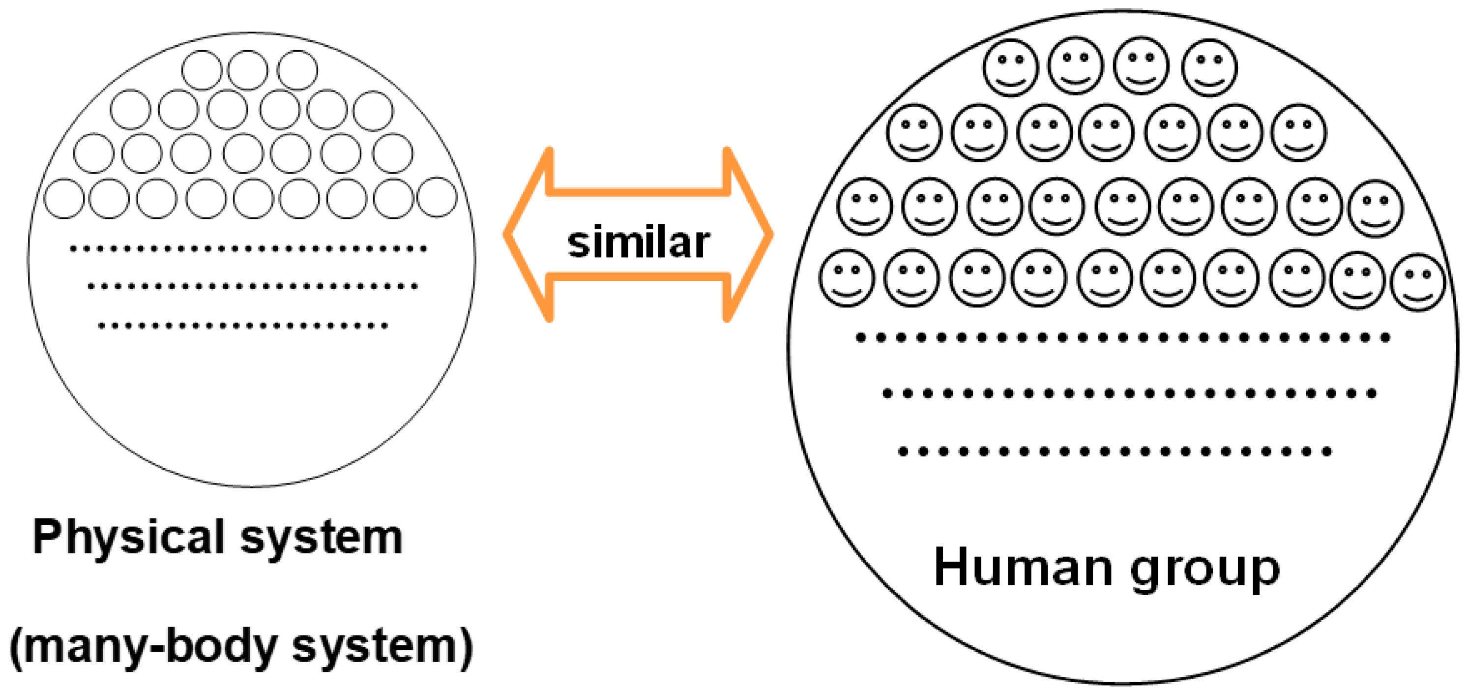
6]. In this case, each opinion is represented relatively simply. Without individual details, there are some similar properties between many-body systems in physics and human groups consisting of many persons (
Figure 1). This means we can get information on human phenomena and discover the features of groups by using statistical mechanics [
7].
Mathematical models whose components have two states are used for various fields as well as physics, for example, neuroscience [
8], sociology [
9] and economics [
10]. The sociological model of these types was originally established by Weidlich in 1971 [
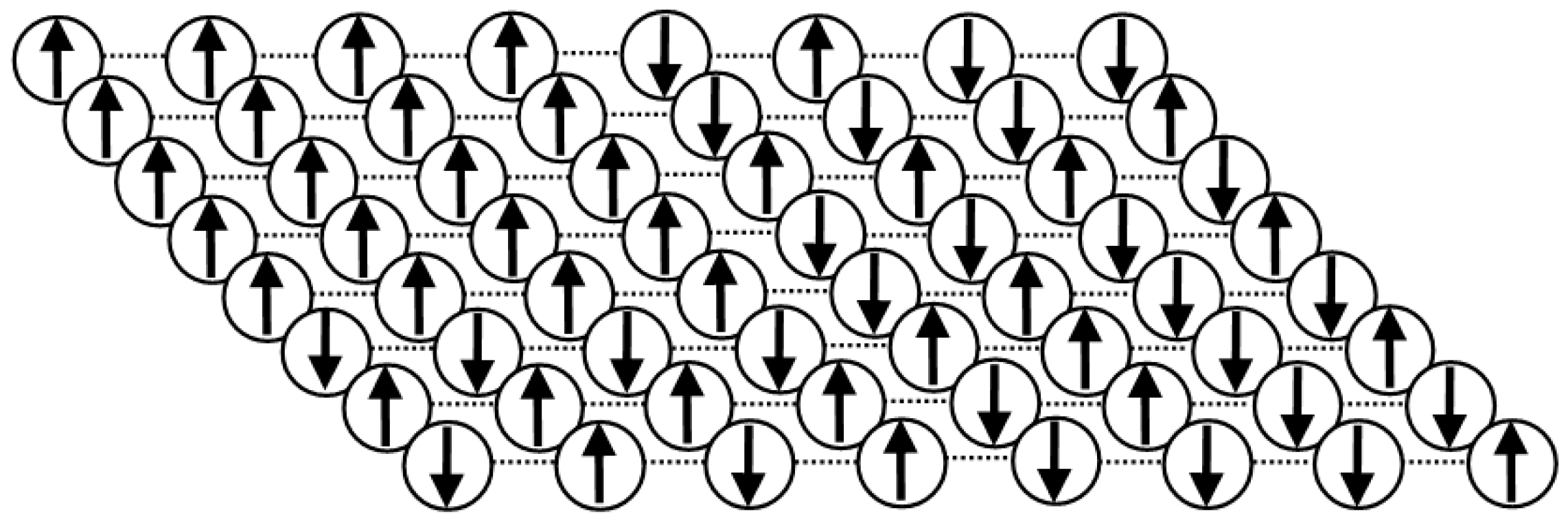
11]. In the framework of synergetics, the Weidlich model was constructed by an analogy between human decision-making mechanisms and the ferromagnetic spin model in statistical physics (
Figure 2). Nowadays, the Weidlich model has many applications [
4,
5].
On the other hand, the order and/or disorder in the many-body system can be expressed by the entropy, a concept proposed by Boltzmann in statistical physics in the nineteenth century [
12]. In the mid-twentieth century, Shannon extended the entropy concept to apply to information theory [
13]. Nowadays, entropy in the information theory has been a powerful tool, applied in many stochastic systems [
14].
Recently, we applied the principle of synergetics to construct a mathematical model of classroom conditions [
15]. In the present study, we develop the model to apply the concept of entropy to discuss classroom conditions. We argue various states of the classroom condition by numerical calculations, which are invisible in the raw data. Thereby, we can obtain a measure of interaction among students, and a measure of moral and entropy in the classroom. In order to confirm the present method, we try to get information on the fluctuation in students’ minds by taking pictures of desk arrangement in each classroom. Also, we gained information by a questionnaire given to students. Analyzing the data, we show that the present method can be a useful tool for educational psychology and management.
2. Methods: Entropy in a Sociological Model of Opinion Decision-Making Processes
A sociological model of opinion decision-making processes has been developed by Weidlich (1971) [
11]. By combining Shannon’s information theory (1948) [
13], we try to obtain entropy in the sociological model of opinion decision-making processes. As preparation for the later discussion, we recapitulate briefly the essential aspects of entropy in the information theory (
Section 2.1) and the Weidlich model (
Section 2.2). We propose the entropy formula of the Weidlich model (
Section 2.3).
2.1. Entropy in the Information Theory
The concept of entropy was originally established in thermal physics. The word “entropy” was first introduced by Clausius in 1864, then the second law of thermodynamics was clearly expressed by entropy. Afterwards, Boltzmann emphasized the probabilistic meaning of entropy, and proposed the expression S = kB logW, which means the disorder of constituents in the system, where W is the total number of possible arrangements of particles and kB is the Boltzmann constant. The increase in entropy S corresponds to the increase in disturbance of the condition of the system.
In the present study, we treat the random phenomena whose results are uncertain before the measurements. The concept of measurement of the uncertainty of random variables is described by “Entropy” in the information theory [
14].
Entropy in the information theory is defined by Shannon, as follows [
13]:
H(
p1, …,
pm) is called “entropy of probability distribution”. We can see that the concept of entropy in the information theory includes the concept in statistical physics. If
pi = 1/
W, Boltzmann’s entropy is the same as Shannon’s entropy, except for a multiple constant, as shown in the following.
In the case of continuous random variables, we need to extend the concept of entropy. Shannon introduced the new concept “differential entropy” [
13], which is an extended concept from entropy in the discrete case. In the continuous case, the probability is expressed by the function
p(
x) on the continuous variable
x. The “entropy” is extended to the following equation, which is called “the differential entropy” of
p(
x).
where
R is a set of real numbers. The differential entropy depends only on the probability density of random variables. However, there are some differences between the continuous and the discrete cases. The most important point is that the differential entropy
Hd (
X) can take negative values, whereas the entropy
H(
X) in the discrete case always satisfies
H(
X) > 0. Although the differential entropy can have not only positive value but also a negative value, it is known that the difference
Hd (
X)
-Hd (
Y) is a meaningful quantity in the system [
14]. That is, the difference
Hd (
X)
-Hd (
Y) means the increase or decrease in disturbance in the system.
2.2. The Weidlich Model for the Stochastic Process on the Change of Opinions
In order to describe opinions in human behavior mathematically, there are many approaches in mathematical modeling in sociology. Focusing the stochastic process on the changes of opinions, we can find an analogy between the human decision-making mechanism and the spin model in statistical physics (
Figure 3). As a matter of fact, Weidlich combined the spin model with the human opinion-making processes.
Thus, the components of the Weidlich model are represented by spin variables of spin up ↑ or down ↓, which correspond to two opposite human opinions. The total number of components (population) is denoted by
n
where
and
are the total number of spin ↑ and ↓, respectively. Although the values of
and
can change, the value of
n does not change, so
n is a conserved quantity in this model. In order to reduce the number of variables in the model, a new variable
x is defined as follows.
In this model, the transition probabilities per unit time for an individual are set up to follow equations by an analogy with statistical mechanics.
where parameter
k is a measure of the strength of adaptation to neighbors;
h is a preference parameter;
ν is a measure of the frequency of the flipping process. The validity of these transition probabilities is recognized in various fields [
4,
5].
In the case of
n >> 1,
x can be regarded as a continuous variable, and this statistical system is described by the probability distribution
f (
x; t), which is determined by a partial differential equation called the “Fokker–Planck equation” (
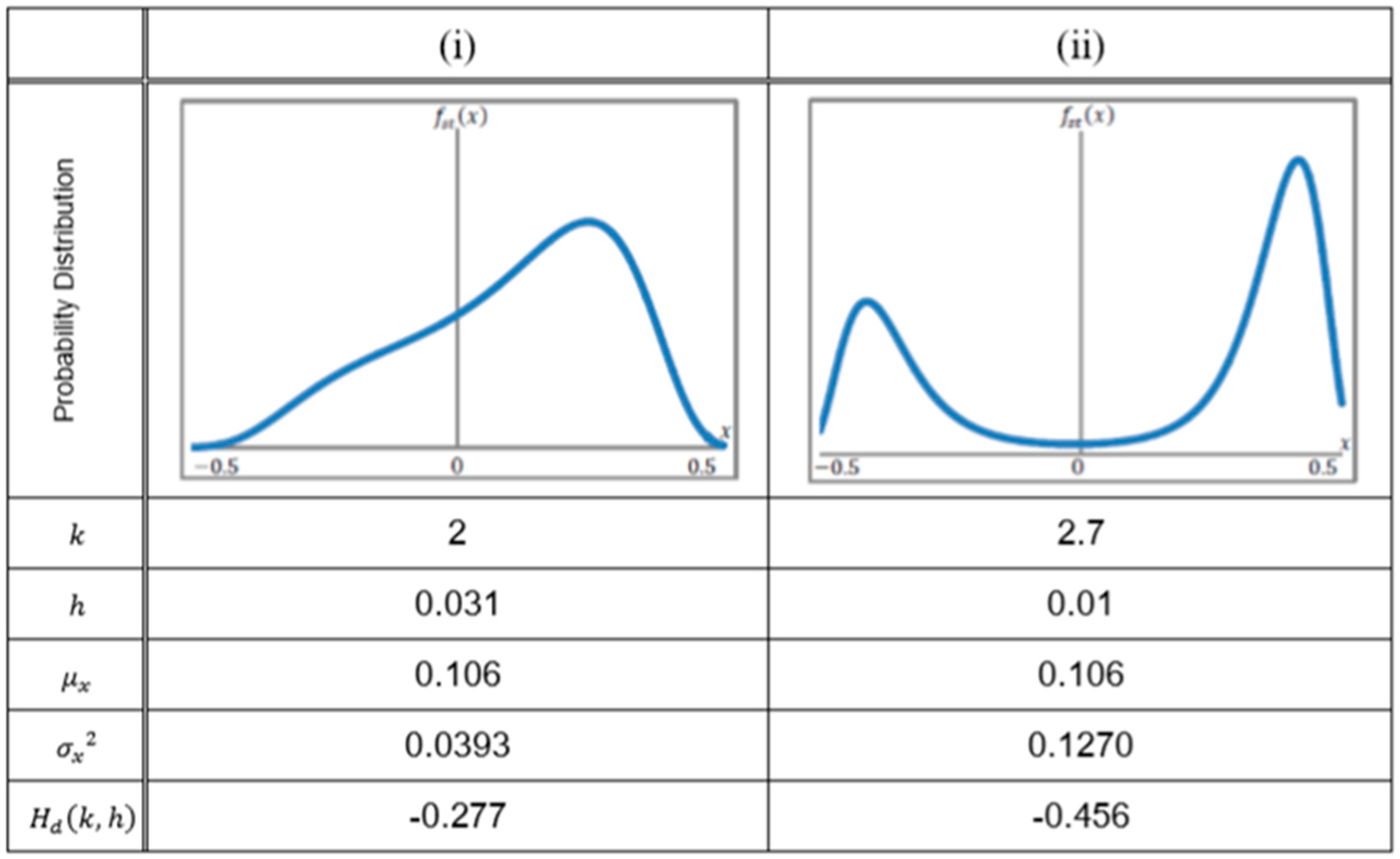
Appendix A). It is proven that the Fokker–Planck equation of the Weidlich model has a time-independent solution which is called “the stationary probability distribution” and denoted by
fst (
x). The parameters
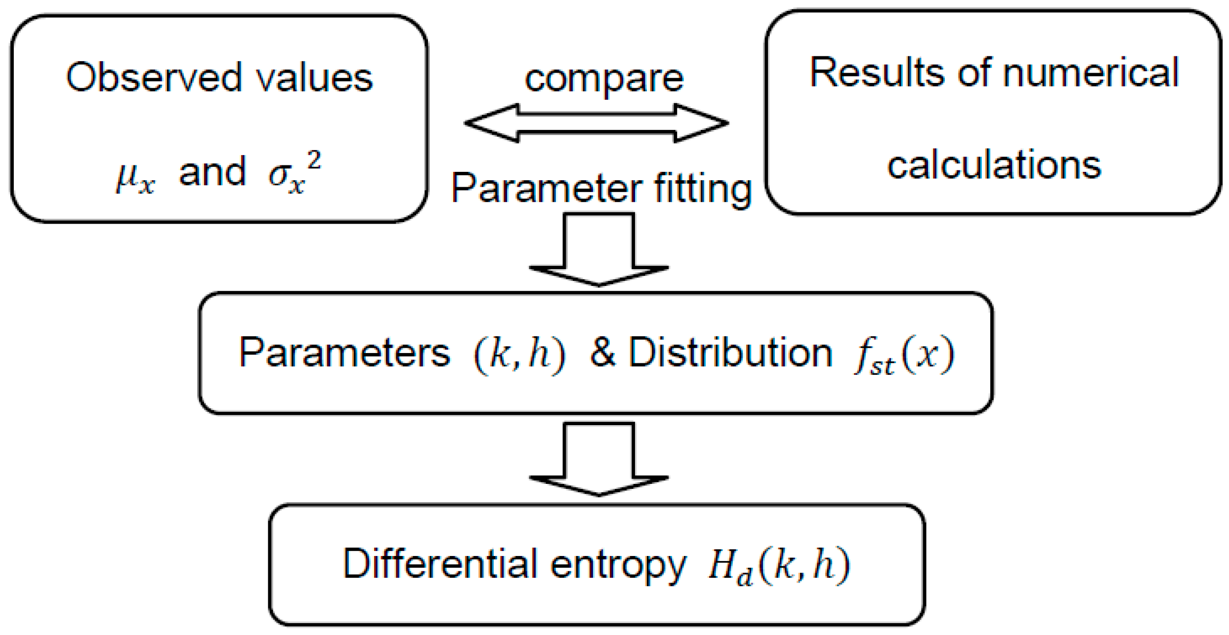
k and
h, on the other hand, are determined by the parameter fitting, comparing the results of numerical calculations with the observed values
μx (the mean value of
x) and
σx2 (variance of
x). Then, the stationary probability distribution
fst (
x) is obtained with the values of
k and
h, as shown in
Figure 4. The details of calculation are described in
Appendix A.
2.3. Differential Entropy of Stationary Distribution on the Weidlich Model
Combining the differential entropy formula and the Weidlich model, we can calculate the differential entropy Hd (k, h) on the stationary distribution fst (x; k, h), which is determined by two parameters of k and h in the Weidlich model, as follows.
The strategy of the calculation of differential entropy with the observed values is schematically summarized in
Figure 4.
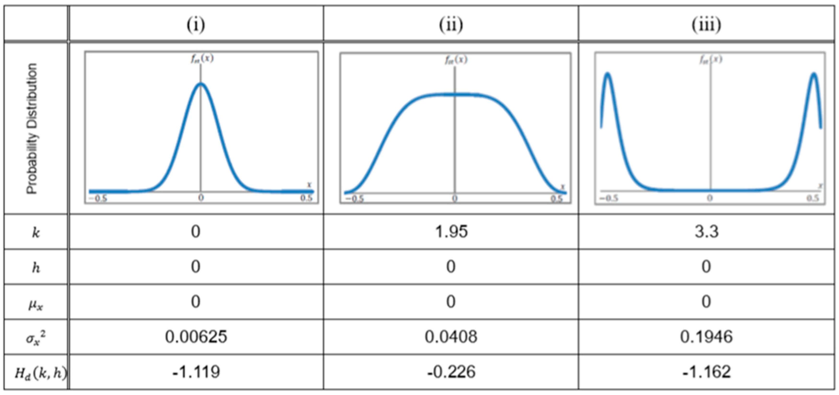
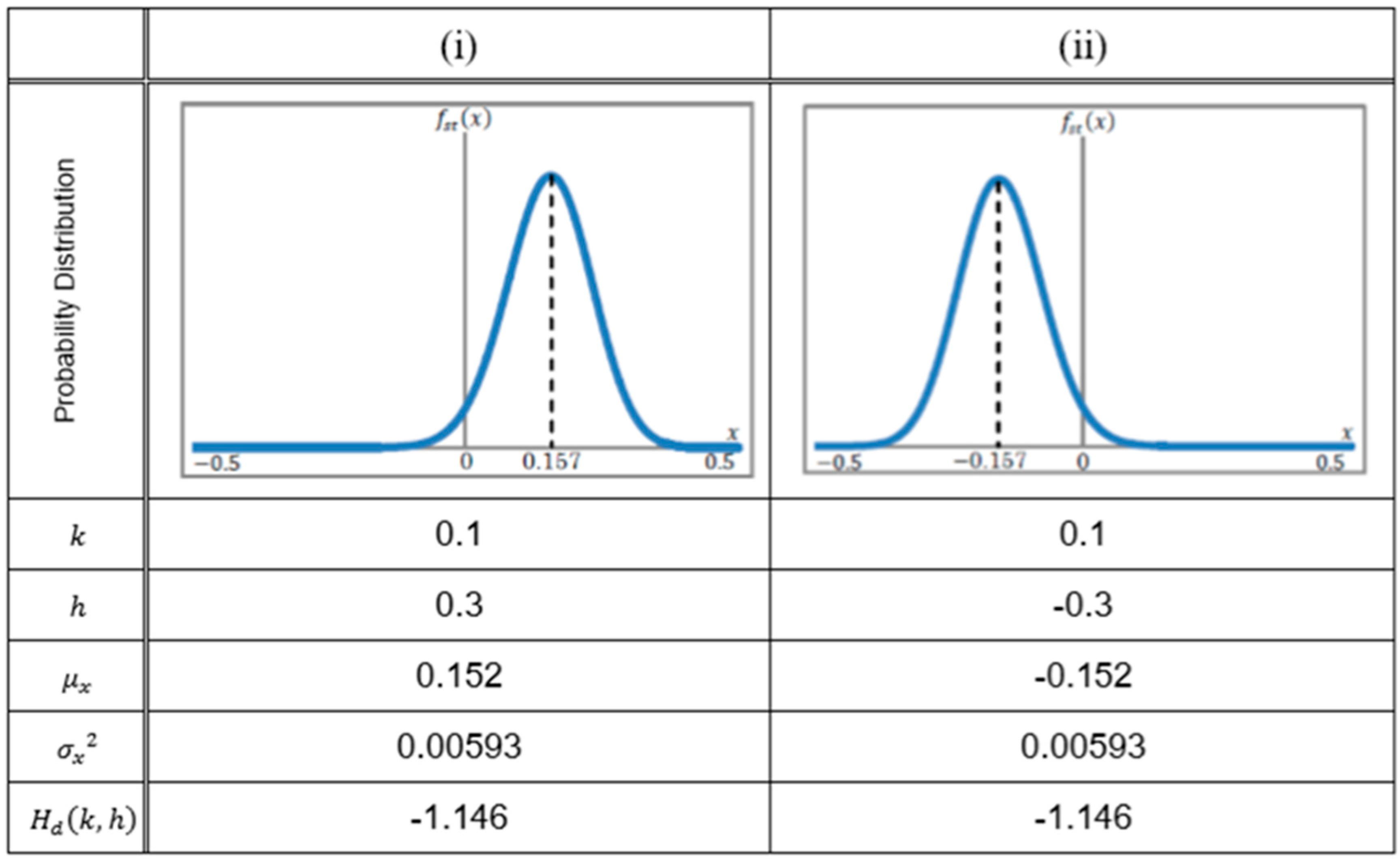
Behaviors of the differential entropy on the Weidlich model are shown in
Appendix B.
3. Materials
Hereafter, we try to apply the method shown in
Figure 4 to classroom conditions. Firstly, we tried to obtain data with different methods of photographing and a questionnaire, relating to the classroom organization in a selection of lower secondary schools in Japan (
Section 3.1). Secondly, we set the obtained data into two state variables (
Section 3.2).
3.1. Data Obtained from Classroom
In the application of the present method, the most difficult point was the selection of data which can show some fluctuations in the students’ minds. In this study, we will adapt the data of “photographing desk arrangements” and “questionnaires”, as described below. The kinds of data were intuitively chosen by the teachers.
For classroom management, we usually pay attention to students’ behaviors to detect the fluctuations in the students’ minds. Most schools adopt school lunch programs, so all students have the same lunch menu in their classroom. Students clean the classroom and other places in their school by themselves. At the start and the end of the day, they have a meeting in their classroom, which is called “Home-Room time”.
The investigations were done for three classes in a lower secondary school in Japan. The members of these classes were usually comprised to have similar scholastic ability and physical strength. The classes were not specially comprised for this investigation. The number of students in each classroom was
n = 39 or 40. The age of students was 12 or 13. The ratio of boy to girl students was approximately 1 to 1 in each classroom. The period of investigation was a successive five days in June, September and December, 2018. It must be noted that the sample size utilized in simulations on the Weidlich model should not be too large. If the sample size is too large, it becomes difficult to see the fluctuations in the data against the parameter. In fact, the sample sizes utilized so far in many simulations on the Weidlich model were between 40 and 50 [
4,
5]. Therefore, the sample size in our research was suitable for the investigation of fluctuations.
Details of the photographing and questionnaires to get information on the fluctuation in students’ minds in each classroom are as follows.
(1) Photographing Desk Arrangements
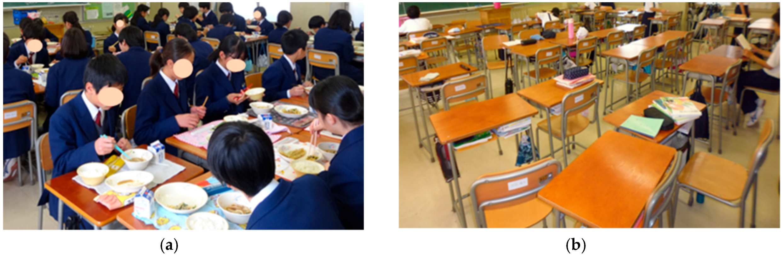
Usually, students have lunch in small groups with seven or eight members, making islands with their desks (
Figure 5a). After lunch, they return to the ordinary desk arrangement (
Figure 5b) for the next lesson. Basically, they must fix the direction of the desks (rearrangement). In order to check the turbulence of desk arrangement, we took the photos a few minutes after lunch, when the rearrangement of the desks for the next lesson was finished. The pictures of classroom were taken from four directions.
(2) Questionnaires
In order to gain information on the fluctuation in students’ minds, from the students’ school life (attitudes in lessons, cleaning, class meetings and so on) other than the rearrangement of desks after lunch time, we utilized questionnaires. Students were asked to fill out five questions in the questionnaire, which relate to their school life. Each item of the questionnaire was answered in the Likert-style 4-point scale format, ranging from 4 (strongly agree) to 1 (strongly disagree). The five questions are as follows:
“Did you calmly spend in every lesson today?”
“Did you do good greetings of the beginning and end in every lesson today?”
“Did you eat all the lunch today?”
“Did you do cleaning earnestly today?”
“Did you participate positively in the Home-Room time today?”
3.2. Setting of Two-States Variables on the Desk Arrangements and the Questionnaires
Each category—the desk arrangements and the questionnaires—was divided into two parts which relate to two states of spin variable ↑ and ↓, described in
Section 2.2. For instance, in the photographic investigation, the state of desks where the angle deviates more than 20 degrees from the right angle were assigned to ↓, and the other states to ↑. In the questionnaires, positive answers and others were assigned to ↑ and ↓, respectively. Setting the two states, the value of x is obtained as described in
Section 2.2.
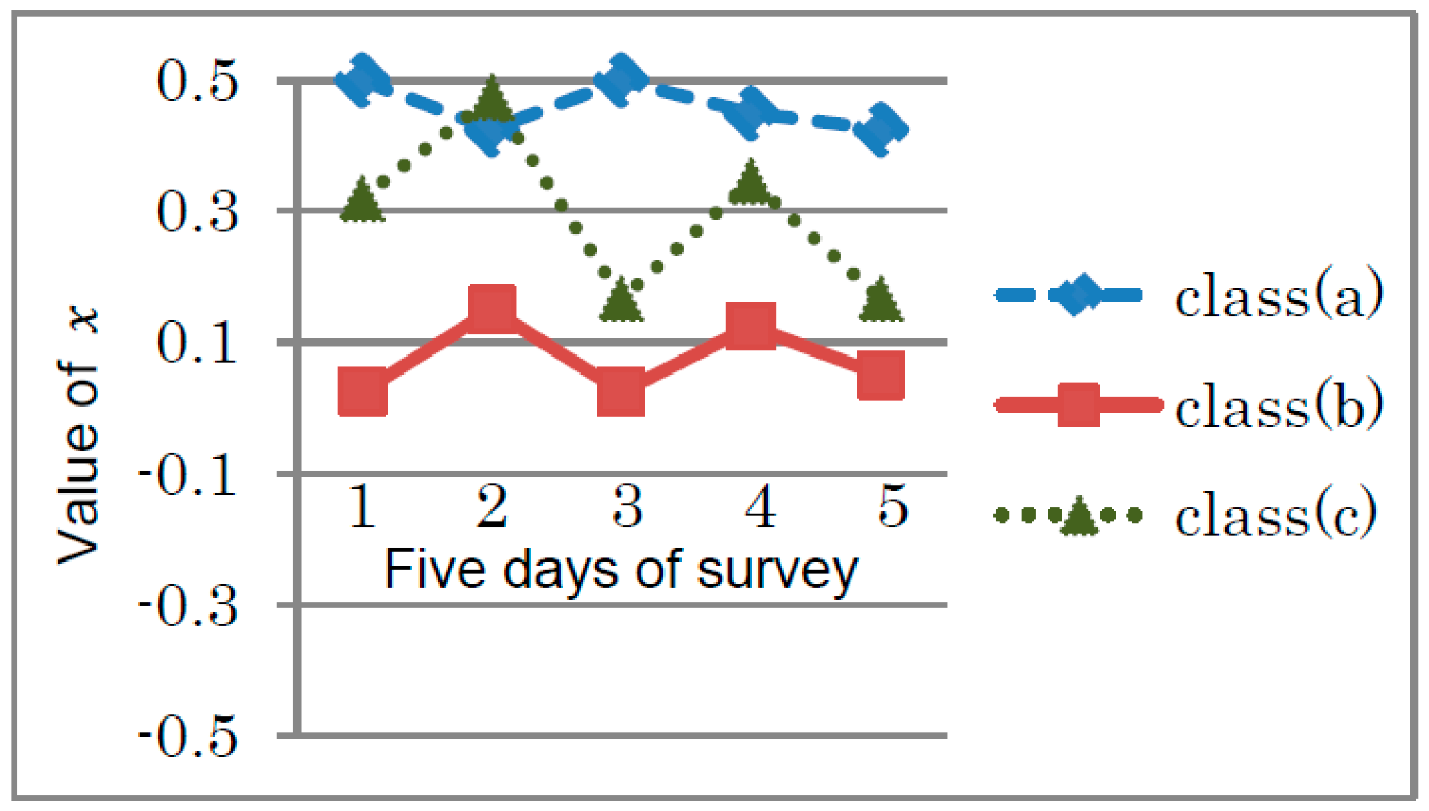
Figure 6 shows the change in the value of x on the desk arrangements over five days in September for the classes (a), (b) and (c).
4. Results: Calculations of (k, h) and Hd (k, h) with the Obtained Data
In this section, we calculate the values of (
k,
h) and the differential entropy
Hd (
k, h) by using the data of the desk arrangements and the questionnaire about attitudes in lessons obtained in
Section 3.
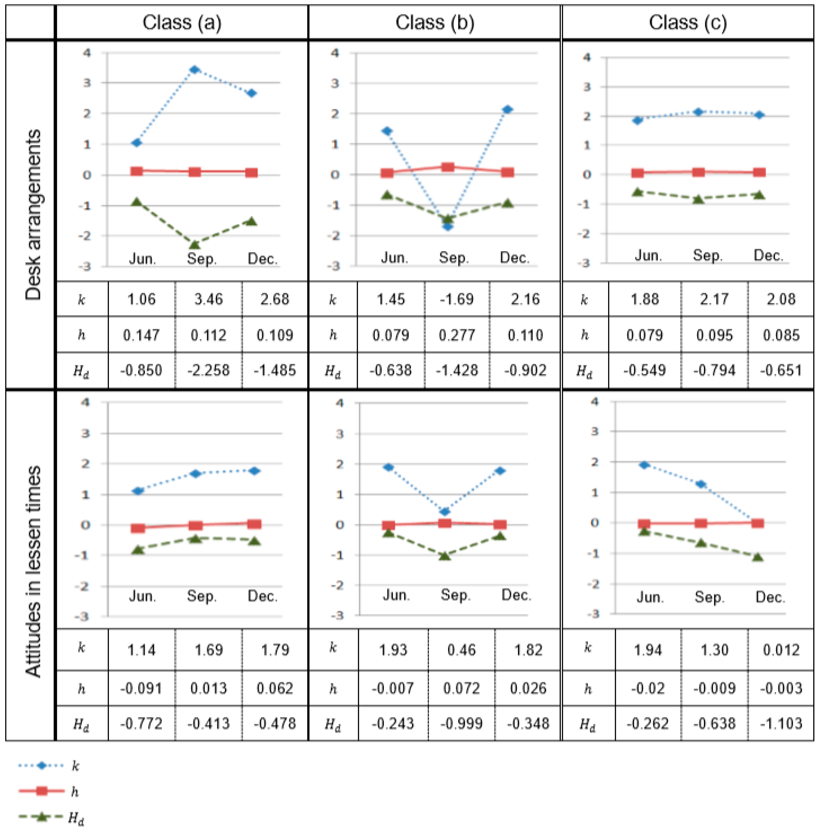
All the results, calculated numerically with the data of desk arrangements and the attitudes in lessons over the successive five days in June, September and December, are shown in
Table 1. The investigations were carried out approximately every three months. The data of other questions in the questionnaire, except for the attitudes in lessons, scarcely expressed fluctuations. The corresponding probability distributions exhibit insignificant features, with almost constant values of
x. Therefore, we utilized just the results of desk arrangements and attitudes in lesson times.
Figure 7 shows the changes in
k,
h and
Hd (
k,
h) over the three months for the classes (a), (b) and (c).
5. Discussion: Classroom Conditions and Calculated Results
In the preceding section, we calculated the values of (k, h) and the differential entropy Hd (k, h) by using the data of the desk arrangements and the questionnaire on attitudes in lessons, where the parameter k is a measure of the strength of adaptation to neighbors and h is a preference parameter. One should note that the parameter h can be interpreted as a “moral parameter”, as all the questions in the questionnaire and the desk arrangements are related to students’ morals. Here, we discuss the relation between the classroom conditions and the calculated results.
In
Figure 7, we can find some differences in the changes in the parameters (
k,
h) and differential entropy
Hd (
k,
h), which are numerically calculated by using the data of the desk arrangements and the questionnaire on attitudes in lessons. A remarkable change can be found in the parameters (
k,
h) and
Hd of Class (b) during September to December. It shows that
k (a measure of the strength of adaptation to neighbors) increases but
h (a moral parameter) slightly decreases, and differential entropy
Hd (mental disorder of the group) increases, in both investigations. This means that the interactions of each member were strong, but their morals were slightly weak, and the mental stability of the group was disturbed.
According to a distinct survey in the end of December 2018, it was revealed that Class (b) had experienced trouble during October to December. That is, bullying occurred in Class (b) in this interval. Specifically, one student was bullied by many students in the class. Other students were not able to stop the trouble because the classroom had an atmosphere in which students could not assert these opinions. Notably, this situation corresponds well to the varying of the value of parameters in
Figure 7, where
k and
Hd increase but
h slightly decreases. The increase of parameter
k means that the interaction force of students becomes strong. The increase in differential entropy
Hd can be interpreted as the increase in the instability of the group. The decrease in parameter
h, on the other hand, means that the morale of students becomes weaker. In this condition, if some negative feelings accidently happen, they will appear as fluctuations, but these should be enlarged by both the increase in
k (interaction force of students) and
Hd (mental disorder of the group). Thus, this situation matches the occurrence of bullying.
Interestingly, the increase in the interaction force of students does not only suggest good conditions in the classroom but also the occurrence of bullying. Therefore, it cannot be always said that the increase in the interaction force of students means there are good conditions in the classroom. In other words, the increase in both k and Hd may be a symptom of bullying. This is similar to a totalitarian society. Thus, in this study, we see some similarities between the classroom and society.
In the present research, we used the data of the desk arrangements and the questionnaire on attitudes in lessons to see the fluctuations in students’ minds. The questionnaire on attitudes may be a useful one, as it has been used in previous research works on creativity [
16,
17]. One should note that the data for the present model could be anything other than the desk rearrangement or the attitudes in lessons, if it shows some fluctuations in the students’ minds. However, the sample size should not become too large, as described in
Section 3.1. In addition, the characteristics of samples may depend on social background, heterogeneity of gender, age, etc. Therefore, further investigations are needed to clarify what type of sample is proper for the present model.
6. Conclusions
In this study, we proposed a novel method to discover classroom conditions by utilizing the concept of entropy and a mathematical model which has not used in educational psychology to date. In order to obtain the entropy of the classroom, we combined the formula of differential entropy and the Weidlich model, which belongs to synergetics. We investigated the usefulness of our approach by using data on students’ lives in school, including photos of the arrangement of desks after lunch and questionnaires on school life. By numerical simulations, the classroom conditions are simply expressed by entropy and two parameters, which are a measure of the interaction of each member and a measure of moral in the group. These quantities are invisible in the raw data but can be deduced by analyzing the present method. Thus, we can numerically argue various conditions of the classroom. Comparing the calculated results with real classroom conditions, we can find good correspondences, and suggest the usefulness of the present method for knowing classroom conditions through rather simple investigations including photography and questionnaires. Nonetheless, our investigation was limited to one case in Japan. Therefore, further investigations are awaited to check the validity of the present novel method. Moreover, further investigations are needed to clarify the best way to choose the proper data for the present method to work with educational, psychological, and sociological theories, since the data was intuitively chosen by the teachers, as described in
Section 3.1. Also, the theoretical framework, which contextualizes the data design and analyses educational discussions on the school climate, effectiveness and classroom management, is the theme of our research in the future.


