Abstract
Extant literature on education research focuses on evaluating schools’ academic performance rather than the performance of educational institutions. Moreover, the State of Louisiana public school system always performs poorly in education outcomes compared to other school systems in the U.S. One of the limiting factors is the stringent standards applied among heterogeneous schools, steaming from the fit-for-all policies. We use a pairwise controlled manifold approximation technique and gradient boosting machine algorithm to typify Louisiana public schools into homogenous clusters and then characterize each identified group. The analyses uncover critical features of failing and high-performing school systems. Results confirm the heterogeneity of the school system, and each school needs tailored support to buoy its performance. Short-term interventions should focus on customized administrative and academic protocols with malleable interpositions addressing individual school shortcomings such as truancy. Long-term policies must discourse authentic economic development programs to foster community engagement and creativity while allocating strategic resources that cultivate resilience at the school and community levels.
1. Introduction
Two reports published in 1983 by National Commission on Excellence in Education and Carnegie Forum on Education and the Economy painted a grim picture regarding education outcomes in the U.S. As a result, states and school districts have implemented policies and regulations to foster high academic standards, improve accountability, and achieve excellence while administering rules and laws to maintain school disciplinary conduct. However, according to [1,2,3], the U.S. still has one of the highest high school dropout rates in developed countries, and among students who complete high school and go on to college, half require remedial courses, and half never graduate [4,5].
For the U.S. youth to compete for rewarding careers against other brilliant young people from across the globe, a college degree or advanced certificate is necessary. As the World Economic Forum reports [6], three-quarters of the fastest-growing occupations require education beyond a high school diploma, with science, technology, engineering, and mathematics (STEM) careers prominent on the list. To reignite U.S. education competitiveness, relight economic growth, and create a thriving middle class, the U.S. requires an inclusive education system that prepares all students for college and STEM careers and implements innovative public policies to ensure every child receives a quality education.
The extant literature related to quantitative (behavioral and cognitive) education analyses focuses on determining factors influencing student achievements and school performance using academic growth models and other econometric tools summarized by [7,8]. These models assume that schools or school systems are homogenous. What arises from these studies are fit-for-all public policies that do not necessarily impact education outcomes, as no one policy guarantees success [6]. Due to location and neighborhood effects, schools exhibit heterogeneous characteristics and face different challenges and constraints across districts and time; therefore, they demand tailored and diversified support.
Most education studies rely on academic growth models [9] to measure students’ progress or schools’ performance on standardized test scores concerning academically similar students from one point to the subsequent and students’ progress toward proficiency standards. These models provide a general framework for interventions to revivify failing students or schools or rally high-achieving students or schools. However, results from these models are not helpful when the objective is deriving tailored recommendations for specific students or schools with distinctive features and characteristics that differ from others. Moreover, the statistical methods for controlling student background and other extraneous variables in these models make it impossible to determine the impact of covariate variables on student or school performance [9,10].
This study deviates from these studies by focusing on whether there is a non-random structure in the Louisiana public school system and pinpointing critical features that differentiate Schools’ performance. In this study, we used pairwise controlled manifold approximation (PaCMAP) as an unsupervised machine learning tool for multidimensionality reduction and visualizing the created school clusters [11] and applied different internal statistical tools to determine optimal numbers of clusters and validate the created groups as reported elsewhere [12]. Further analysis using visualization tools and multiclass classification, specifically random forest and gradient boosting machine method [13], identifies critical features of failing and performing schools. The results are vital in suggesting tailored interventions to improve Louisiana’s public school system’s performance.
Figure 1 presents the steps taken for data collection and analysis, and the study has two main contributions. First, the unsupervised clustering technique illustrated in Figure 1 below helped build a multiclass classification model based on historical data to predict which schools belong to what cluster and what features are essential in each homogenous group. Therefore, school administrators and policymakers can respond appropriately to target certain shortcomings at the school level.
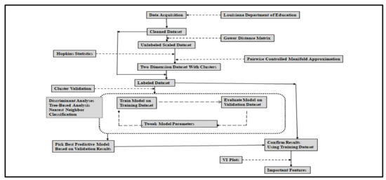
Figure 1.
Machine learning steps to typify the schools and identify critical features.
The analysis illustrated in Figure 1 allowed a simultaneous utilization of unlabeled and labeled data and enabled tracking of the effects of distinctive features on cluster projection. Second, combining unsupervised and supervised clustering tools allowed us to compare features across clusters that uncover connections between school characteristics and performance and critical differences among schools. The results provide evidence-based decision-making tools for selecting and implementing interventions to improve school outcomes. As illustrated in Figure 1, we use unsupervised machine learning techniques [14]; explicitly, we cluster schools into sub-homogenous groups using PaCMAP [11] and identify critical features of each cluster using multiclass classification [13,15]. Data points in clusters should be as similar as possible and dissimilar to teams in other groups. The main advantage of clustering is its adaptability to changes, which helps single out valuable features that distinguish distinct groups. Moreover, grouping schools by commonalities or differences is essential in exploring the factors that explain differences in achievement and performance. Clustering also helps to understand existing challenges and opportunities that influence change.
While the best clustering process maximizes inter-cluster distances, it should also minimize intra-cluster distances [16] (Bailey, 1989). The inter-cluster distance (global structure) is the distance between two data points belonging to different clusters, and the intra-cluster distance (local structure) is the distance between two data points belonging to the same group. A superior clustering algorithm makes clusters so that the inter-cluster distance between different clusters is prominent and the intra-cluster space of the same group is conservative. Popular methods for clustering social data through multidimensional reduction techniques include fuzzy clustering [17], t-distributed stochastic neighbor embedding (t-SNE) [18,19], uniform manifold approximation and projection (UMAP) [20], dimensionality reduction using triplet constraint (TriMap) [21]. The primary limitations of these methods are that they either preserve local or global structures, and hyperparameters of the models are difficult to interpret [11]. The PaCMAP is an ideal tool for clustering through dimensionality reduction as it depends on a founded mathematical formulation. Moreover, PaCMAP uncovers strong connections among variables by safeguarding local and global structures, an essential aspect of the geometric visualization of multidimensional datasets [11,22].
Evaluating the dimensionality reduction and cluster analysis includes quantitative and objective ways through cluster validation measures. The process has four main components: determining whether there is non-random structure in the data; determining the optimal number of clusters; evaluating how well a clustering solution fits the given data when the data is the only information available; and assessing how well a clustering solution agrees with partitions obtained based on other data sources. The first step involved evaluating the clustering tendency before applying the dimensionality reduction and clustering algorithms to determine whether the data contains any inherent grouping structure using the Hopkins statistic [23]. The statistic evaluates the null hypothesis that the data follows a uniform distribution (spatial randomness). In the second step, we used clustering validation measures [24,25] to determine the goodness of a clustering structure without respect to external information.
We organize the remaining part of the paper into four sections. The following section is the literature review that focuses on popular clustering techniques, their limitations, and the fundamentals of multiclass classification using machine learning. The data source, descriptions, and rationale of variables used to cluster the school systems and specific empirical techniques for data analysis are in Section 2, followed by the results and discussion section and the last section on implications for short- and long-term policies.
2. Background Information and Literature Review
2.1. Louisiana Schools Accountability System
According to the Louisiana Department of Education [26,27], the accountability system of the Louisiana school system aims to inform and focus educators through clear expectations for student outcomes; and provide objective information about school quality to parents, community members, and other stakeholders. Annually, public schools and early childhood centers in Louisiana receive a performance report that measures how well they prepare their children for the next phase of schooling. Since 1999, the state has issued public school performance scores (SPS) based on student achievement data. To communicate the quality of school performance to families and the public, Louisiana adopted letter grades (A–F). In 2014, the Department recalibrated its school performance score scale from a 200-point scale to a 150-point scale.
Under the previous 200-point scale, the letter grade was: A (120–200), B (105–119.9), C (90–104.9), D (75–89.9, F (0–74.9), and T (turnaround school). Under the 150-point scale, the groups of SPS are as follows: A (100–150), B (85–99.9), C (70–84.9), D (50–69.9), F (0–49.9), and T (turnaround school). The SPS for elementary is estimated based on these subindices: assessment (70%), growth (25%), and interest and opportunities (5%). The assessment subindex includes student assessments in student learning in English language arts (ELA), math, science, and social studies to measure student proficiency in the knowledge and skills reflected in the standards of each grade and subject. The SPS includes the points assigned to achievement levels by students for each subject assessed and progress made toward English language proficiency.
The calculation of the growth index accounts for changes in schools’ performance based on the previous year and the current year’s scores on each assessment result. Assessing student growth is done by answering two questions. If students are not yet achieving proficiency, are they on track to do so? If a student reaches the target, the school earns 150 points. Otherwise, if the students are growing at a rate comparable to their peers, schools earn points based on students’ growth percentile as compared to peers (i.e., 80th –99th percentile (150 points), 60th–79th percentile (115 points), 40th–59th percentile (85 points), 20th–39th percentile (25 points), and 1st–19th percentile (0 points). In addition, the interest and opportunities subindex constitutes a 5-point scale on various metrics reflecting the schools’ effort to make services available to all children.
Based on the Louisiana Department of Education [28], the SPS for elementary/middle schools with grade 8 is an aggregation of these subindices: assessment (65%), achievement and growth (25%), interest and opportunities (5%), and dropout credit accumulation (5%). For the high schools, the SPS is also an aggregation of the following subindices: assessment (25%), ACT/WorkKeys (25%), the strength of diploma (25%), cohort graduation rate (20%), and interest and opportunities (5%). The assessment subindex for the high schools includes the end-of-course (EOC) exams that assess whether students have mastered the standards of core high school subjects. EOC exams include algebra I, geometry, English I (beginning in 2017–2018), English II, biology, and U.S. History. Except for students who participate in LEAP alternative assessment 1, all high school students must take an ELA and math EOC exam by their 3rd cohort year, regardless of graduation pathways. The final scores do not include high school students retaking an EOC. Final student scores are on five levels: unsatisfactory (0 points), approaching basic (50 points), basic (80 points), mastery (100 points), or advanced (150 points). The mastery and above are considered proficient for the next grade level.
The dropout credit accumulation subindex is for schools that include grade 8 in the prior year, based on the number of Carnegie credits earned through the end of 9th grade (and transitional 9th, where applicable) and/or dropout status. The dropout credit accumulation encourages the successful transition to high school and access to Carnegie credits in middle school. The ACT/WorkKeys (ACT WorkKeys assessments are the cornerstone of ACT workforce solutions and measure foundational skills required for success in the workplace and help measure the workplace skills that can affect job performance) subindex measures student readiness for postsecondary learning, and all grade 11 take the ACT, a nationally recognized college and career readiness measure. Schools earn points for the highest composite score made by a student through the spring testing date of their senior year or a student who graduates at the end of grade 11. WorkKeys scores were included in the ACT subindex for accountability when the WorkKeys score yielded more index points than the ACT score beginning in 2015–2016.
Louisiana Department of Education report [27] indicates that the Strength of Diploma subindex measures the quality of the diploma earned by each 12th grader. The high school diploma plus awards points (110–150)) to schools for students who graduate on time and meet requirements for one or more of the following: advanced placement, International Baccalaureate (IB), JumpStart credentials, CLEP, TOPS-aligned dual enrollment course completion, and an associate degree. The system awards schools with four-year graduate students (100 points) with career diplomas or a regional Jump Start credential, as well as those who earned a diploma assessed on an alternate certification. Moreover, the system awards 50–75 points to schools with five-year graduates that have any certificate, five-year graduates who earn an A.P. score of 3 or higher, an IB score of 4 or higher, and a college-level examination program (CLEP) of 50 or higher. Other awards are for graduates with high school equivalency test (HiSET)/GED + JumpStart credential (40 points), and HiSET/GED earned no later than October 1 following the last exit record (25). The cohort graduation rate subindex measures the percentage of students who enter grade 9 and graduate four years later, adjusted for students who transfer in or out. All 9th-grade students who enter a graduation cohort are included in the cohort graduation rate calculations, regardless of diploma pathway, unless they are legitimate leavers. Legitimate leavers are students removed from the cohort and exited enrollment for one or more reasons: death, transfer out of state, transfer to an approved nonpublic school or a Board of Elementary Education and Secondary Education)-approved home study program, and transfer to early college.
After the calculation of SPS, the Louisiana Department of Education [27,28] categorize school that needs interventions into three groups: urgent intervention is necessary, urgent intervention is required, and comprehensive intervention is required. For schools in the first category, the subgroup performance equals D or F in the current year. For the second and third categories, the subgroups’ performance equal to F for two years and or out-of-school suspension rates more than double the national average for three years, and the overall performance of D or F for three years (or two years for a new school) and or graduation rate less than 67 percent in most recent year, respectively. For accountability purposes, Comprehensive Intervention Required labels will appear on the “Overall Performance” page in the Louisiana School Finder, while Urgent Intervention Needed and Required labels will appear on the “Discipline and Attendance” and or “Breakdown by Student Groups” pages. As part of Louisiana’s Every Student Succeeds Act (ESSA) plan, any school identified under one of the labels must submit an improvement plan to the Department and an application for funding to support its implementation (See details on how to calculate the SPS at: https://www.louisianabelieves.com/measuringresults/school-and-center-performance (accessed on 17 October 2022)).
2.2. An Overview of Empirical Clustering Techniques and Application in Education
Louisiana’s SPS is an aggregation indicating Schools’ overtime achievement and growth. Analyzing SPS data would allow identifying required changes to improve Schools’ performance. Standard education models used to measure achievement and growth range from subtracting last year’s test score from this year’s test score (called a gain score) to complex statistical models that account for differences in student academic and demographic characteristics [7,8]. The five standard growth models for measuring performance or progress: value-added, value table, trajectory, projection, and student growth percentile. The primary limitations of these models emanate from their inability to account for unobserved characteristics, and there is also a need to specify the mathematical relationship among variables explicitly. However, the education assessment literature (such as [29]) shows no consensus on the best methods and models for evaluating academic achievement and growth at the student and school systems level.
Clustering is a critical technique in data mining with applications in image processing, diagnosis systems, classification, missing value management and imputation, optimization, bioinformatics, and machine learning [30]. Moreover, dimensionality reduction is a fundamental step for clustering algorithms due to the curse of dimensionality and non-linearity of most observational data. As the number of dimensions increases, data points tend to be similar, and there is no clear structure to follow when grouping these pairs [31]. Since cluster analysis is just a statistical process of grouping related units into sets, the groups in the dataset may be genuinely related or related by chance. Different clustering techniques might give different results if the relationship is just by chance [32].
Conventional clustering algorithms such as the k-means clustering technique [33,34] assign a set of observations to a limited number of clusters such that pairs belonging to the same group are more like each other than those in other groups. The method assigns each observation to one and only one cluster. However, the assignment might often be too strict, leading to unfeasible partitions [35,36]. Fuzzy sets manage the challenges by assigning data points to more than one cluster [17]; therefore, each data point has a likelihood or probability score of belonging to a given cluster [37,38,39]. Extensions of the fuzzy c-means clustering algorithm (including [40,41,42]) improve the standard method by reducing errors during the segmentation process.
Education studies (including [43,44]) apply fuzzy clustering to analyze e-learning behavior by creating clusters with common characteristics, typifying schools across cultures [45], or combining learning and knowledge objects based on metadata attributes mapped with various learning styles to create personalized and more authentic learning experiences [46]. Others applied the technique to compare e-learning behaviors [47], predict and identify significant variables that affect undergraduate schools’ performance [48,49], allocate new students to homogenous groups of specified maximum capacity, and analyze the effects of such allocations on students’ academic performance [50], and creating performance profiles in reading, mathematics, and science [51]. Fuzzy clustering techniques perform poorly on data sets containing clusters with unequal sizes or densities, and the method is sensitive to outliers [52]
The t-distributed stochastic neighbor embedding (t-SNE) is a dimension reduction technique that tries to preserve the local structure and make clusters discernible in a two-or three-dimensional visualization [18,53]. The t-SNE algorithm preserves the local structure of the data using a heavy-tailed Student-t distribution to compute the similarity between two points in the low-dimensional space rather than a Gaussian distribution. A heavy-tailed Student-t distribution helps address crowding and optimization problems. The t-SNE algorithm takes a set of points in a high-dimensional space and finds an optimal representation of those points in a lower-dimensional space. The first objective is to preserve as much significant structure or information present in the high-dimensional data as possible in the low-dimensional representation. The second objective is to increase the data’s interpretability in the lower dimension space by minimizing information loss due to dimensionality reduction [54].
Education-related studies use the t-SNE algorithm to predict schools’ academic performance and evaluate the impact of different attributes on performance to identify at-risk students [54] or visualize clusters with unique features that correlate with success in medical school [55] to uncover success potential after accounting for inherent heterogeneity within the student population. Other studies [55] combine convolutional neural networks to identify critical features influencing academic performance and predicting future educational outcomes by visually distinguishing homogenous groups with fully connected layers of the networks [56] and highlighting prominent features influencing education outcomes and predicting future performances [57].
There are two primary limitations when using t-SNE for multidimensionality reduction and clustering. The technique requires calculating joint probability among all data points (at high and lower dimensions), which imposes a high computational burden [11,58]. Therefore, the t-SNE algorithm does not scale well for rapidly increasing sample sizes outside the computer cluster. Also, the algorithm does not preserve global data structure at high dimensions, meaning that only intra-cluster distances are meaningful and do not guarantee inter-cluster similarities [59,60].
Uniform manifold approximation and projection (UMAP) is a non-linear dimension reduction technique used for visualization like t-SNE, with the capacity to preserve local and global structures for non-noisy data [11]. Specifically, UMAP is highly informative when visualizing multidimensional data [61] and performs better in keeping global structure than t-SNE. The UMAP algorithm efficiently approximates k-nearest-neighbor via the nearest-neighbor-descent algorithm [20,62,63]. The application of the UMAP algorithm in education studies identifies community conditions that best support universal access and improved outcomes in the initial stages of childhood development or captures the neighborhoods that behave similarly at a particular time and explains the social-economic effects that bring communities together [22,64,65].
Dimensionality reduction using triplet constraint (TriMap) uses triplet (sets of three observations) constraints to form a low-dimensional embedding of a set of points [11,63]. The algorithm samples the triplets from the high-dimensional representation of the data points, and a weighting scheme reflects each triplet’s importance. The main idea is to capture higher orders of structure with triplet information (instead of pairwise information used by t-SNE and UMAP) and minimize a robust loss function for satisfying the chosen triplets, thereby providing a better global view of the data [63]. Theoretically, this method can preserve local and global structures; however, the inter-cluster distances are uncertain for large datasets with outliers [11,64].
Likewise, PaCMAP is a dimensionality reduction method that preserves local and global data structures [11,29]. The critical steps with the PaCMAP algorithm are graph construction, initialization of the solution, and iterative optimization using a custom gradient descent algorithm PaCMAP. The algorithm uses edges as graph components and distinguishes between three edges: neighbor pairs, mid-near pairs, and further-apart pairs. The first group consists of neighbors from each observation in the high-dimensional space. The second group consists of mid-near teams randomly sampling from additional data points and using the second smallest for the mid-near pair. The third group consists of a random selection of further data points from each observation. Parameters that specify the ratio of these quantities to the number of nearest neighbors determine the number of mid-near and further-apart point pairs. The PaCMAP algorithm is robust and works well on a large dataset, significantly faster than t-SNE, UMAP, and TriMap [65]. We could not find publications related to Education Research that use TriMap and PaCMAP as the primary data analysis tools.
Before clustering, it is critical to determine if the data are clusterable by applying the Hopkins statistic [66] that tests the spatial randomness of the data by measuring the probability that a given data set is from a uniform distribution. The Null hypothesis is that there are no meaningful clusters, and the alternative hypothesis is that the data set contains significant clusters. In addition, while the multidimensional reduction results help identify optimal numbers of clusters through visualizations, the analysis must be augmented by statistical tools such as the Elbow Method [67], the Silhouette Coefficient [68], Gap statistic methods [69], and other statistical measures (summarized by [70]) to ascertain the results. After determining the optimal number of clusters, clustering validation is also vital in deciding group quality [71]. Internal clustering validation aims to establish if the average distance within-cluster is small and the average distance between clusters is as significant as possible [25]. Internal clustering measures reflect connectedness, compactness, and the separation of the created clusters [72].
The connectivity has a value between zero and infinity. Minimizing the connectedness relates to what extent data points are in the same cluster (cohesion) as their nearest neighbors in the data space as determined by the K-nearest neighbors [73]. The compactness index assesses cluster homogeneity using the intra-cluster variance. It measures how closely related the data points in a cluster are. The index is estimable based on variance or distance. Lower variance indicates better compactness [25]. Separation quantifies the degree of separation between clusters by measuring the distance between cluster centroids [38,68]. Compactness and separation demonstrate opposing trends. While compactness increases with clusters, separation decreases with the number of clusters. Most measures of internal cluster validation, such as the Dunn Index and Silhouette width, combine compactness and separation into a single score [25,73]. The Dunn Index is the ratio of minimum average dissimilarity between two clusters and maximum average within-cluster dissimilarity. Given the formula for estimating the Silhouette [68], a Silhouette width for each data point can be positive or negative. Datapoints with a Silhouette close to one are close to the cluster’s center, and data points with a negative Silhouette value mean that the data points are on the boundaries and are more relative to the neighboring groups or clusters [74,75].
2.3. Multiclass Classification to Augment Clustering Results
After unsupervised clustering, the second interest is determining which features/variables significantly impacted each cluster using the original data. The most prominent impact features must differentiate the groups most strongly. Statistically, it is possible to perform a series of analyses of variance and select the attributes/variables with large t-values or smaller p-values [76]. It is also possible to distinguish critical features by calculating the average similarity of each data point based on intra- and inter-cluster distances of the centroid of each cluster [77]. However, a substitution effect occurs when two or more explanatory variables share information or predictive power. The analysis of variance and similarity analysis may not robustly determine which variables are critical [78]. Specifically, multiclass classification is a problem with more than two classes or clusters, where each data point belongs to one category [79]. The technique includes binary classification, discriminant analysis [80,81], tree algorithms extendable to manage multiclass problems, and nearest neighbors’ approach [82]. Discriminant analysis [83] is a versatile statistical method often used to assign data points to one group among known groups. The discriminant analysis aims to discriminate or classify the datasets based on more than two groups, clusters, or classes available priori. The process places new data points into a general category based on measured characteristics. Standard tools for noisy and high-dimensional data are penalized linear discriminant [84], high dimensional discriminant analysis [85], and stabilized linear discriminant analysis [86].
The tree-based algorithms are primary tools for supervised learning methods that empower predictive models with high accuracy, stability, and ease of interpretation. The most popular tree-based algorithms are decision trees [87,88], random forest [89], and gradient-boosting machines [90], as applied by [91,92,93]. Unlike other machine learning models, the algorithm has the quickest way to identify the most significant relationships between variables. Since it is a non-parametric method, it has no assumptions about space distributions and classifier structure [87]. The nearest neighbors’ classification algorithm assumes that similar objects exist in proximity or near each other, and the standard algorithms are the k-nearest neighbors [94] and the nearest shrunken centroids [95]. The objective is to find a group of k data points in the training dataset closest to the test dataset point and label assignments on the predominance of a particular class in this neighborhood. The output is a class membership, assigning each data point to a specific cluster by a plurality vote of its neighbors [94] or earmarked to the class most common among its nearest neighbors.
There are different metrics for comparing the performance of multiclass models and analyzing the behavior of the same model by tuning various parameters. The metrics are based on the confusion matrix since it encloses all the relevant information about the algorithm and classification rule performance [96]. The confusion matrix is a cross table that records the number of occurrences between observed classification (e.g., unsupervised machine learning) and the predicted classification (e.g., from supervised machine learning). Estimable metrics from the confusion matrix dictating more is better (should be maximized) include accuracy, kappa, mean Specificity, and mean recall, and the standard metrics for lower is better (should be minimized) are the logloss and mean detection rate [97]. Generally, the standard accuracy metric returns an overall measure of how much the model correctly predicts the class based on the entire dataset. Therefore, the metric is very intuitive and easy to understand. Balanced accuracy (mean recall) is another critical metric in multiclass classification and is an average of recalls. For details on various metrics used in machine learning model evaluations, see [97,98,99].
After determining the best model, the next step is estimating the relative importance of input variables through k-fold validation [100]. The process identifies the relative importance of explanatory variables by deconstructing the model weights and determining the relative importance or strength of association between the dependent and explanatory variables. For decision tree-based models, the connecting weights are tallied for each node and scaled close to all other inputs. Note that the model weights that connect variables in decision tree-based models are partially analogous to parameter coefficients in a standard regression. The model weights dictate the relative influence of information processed in the network by suppressing irrelevant input variables in their correlation with a response variable. Since no multiclass method outperforms others, the model choice depends on the desired precision and the nature of the classification problems. Therefore, a feature importance score ensures the interpretability of complex models as it quantifies information a variable contributes when building the model and ranks the relative influence of the variable in predicting a specific cluster [101,102,103].
3. Materials and Methods
3.1. Source of Data
This study used data from the 2015/16, 2016/17, and 2017/18 school years. While most data are available up to 2019/20, the financial data was not available when finalizing this paper. All data are from the Louisiana Department of Education Data Center. The link https://www.louisianabelieves.com/resources/library/student-attributes (accessed on 17 October 2022) provides data on schools’ attributes, including the total numbers of students and the percentage of students by gender and race (i.e., American Indian, Asian, Black, Hispanic, Hawaiian/Pacific Islander, and White). Other information is on English proficiency (e.g., percent of fully proficient students), the number of students in different grades, and the percentage in free and reduced lunch programs.
The annual financial report at https://www.louisianabelieves.com/data/310/ (accessed on 17 October 2022) summarizes financial activities for the school year. The variables in the dataset are current expenditures per pupil on instructors, pupil/instructional support, school administration, transportation, and other supports. Other information is on school-level student counts and school-level staff full-time equivalent (FTE) for teachers, administrators, other instructors, and other support staff. There is also information on staff salaries, education levels and average years of experience. The link https://www.louisianabelieves.com/resources/library/fiscal-data (accessed on 17 October 2022) has other financial data summarized by expenditure in each group (e.g., wages, transportation). The link https://www.louisianabelieves.com/resources/library/performance-scores (accessed on 17 October 2022) provides information on school-level performance scores. At the beginning of this study, the scores were available from 1998/1999 to the 2017/18 school year. The full dataset with all variables is available for public schools governed by a school district. School districts with high numbers of private and charter schools that are publicly funded but operated by independent groups, such as in New Orleans Parish, are underrepresented. The New Orleans School District follows the all-charter system with very few schools run by public school systems, and the district is represented by 14 individual schools in the data set. For data analysis purposes, the dataset is in three groups: elementary/middle (elementary after that), combination (with elementary, middle, and high schools), and high schools’ system. The available data are pre-COVID-19 pandemic. Further analysis is needed when the data collected during the pandemic is available, as there is a lag of three years.
3.2. Variables That Influence School Performance and Empirical Model
For definitions and examples of variables that influence school performance, see [104,105,106] on the critical school characteristics and roles of past achievement. Since Schools’ performance depends on schools’ performance, variables influencing school performance are in six groups [107]: schools’ socioeconomic status, past achievement, school attributes, faculty education, per-pupil expenditure, and variables defining the affluence of the communities in school catchment areas. Studies examining the importance of teacher training, teacher certification, and teachers’ professional development programs all conclude that students with certified teachers performed better ([for example, see [108,109,110,111]). Education studies link teachers’ effectiveness to positive student behavior, such as student attendance, which improves schools’ performance [112,113,114]. Other studies examine a constellation of teacher-related effects such as classroom effectiveness, collective teaching quality, and school academic organization that increase student performance and academic growth [115,116,117,118]. Studies (including [119,120,121,122,123]) focus on the influence of class size on student performance with varying conclusions.
Financial expenditure is another variable purported to influence school performance [120,124,125,126,127]; however, the conclusions from these studies are indeterminant. In addition, meta-analysis reviews of quantitative research documenting the association between neighborhoods and educational outcomes all concluded that individual academic results were significantly associated with neighborhood characteristics such as poverty, a poor educational climate, the proportion of ethnic/migrant groups, and social disorganization and other built environment that promotes parental engagement and participation [128].
The variables that capture community affluence are from the five-year American Community Survey (According to the U.S. Bureau of Census, the American Community Survey (ACS) helps local officials, community leaders, and businesses understand the changes in their communities. It is the premier source for detailed population and housing information about the U.S.) at the unified school district level. The data are available from 2009 to 2019 and match the schools’ data. All analyses were in R Environment [129]. To conduct PaCMAP while preserving the local and global structures, we follow a two-step cluster analysis [63] that allows variability among the created clusters [130]. The first step involved calculating Gower’s distance matrix in separating schools into (dis)similar groups using the daisy function in the cluster package [131] (see [132,133] regarding the advantages of Gower’s distance matrix). For PaCMAP, we recreated and executed Python’s pacmap function [11] using a reticulate package [134] in the R environment, the input being the Gowers distance of each school system. Fine-tuning the pacmap function requires specifying the size of the local neighborhood or the number of neighboring sample points (n-neighbors) used for manifold approximation. Larger values result in more global views of the manifold, while smaller values preserve local data. The number of neighbors should range from 2 to 100, but we set it to “NULL” to let the algorithm determine the optimal number of neighbors. Principal component analysis initialized the lower-dimensional embedding at the default levels.
We also used PaCMAP results to identify the medoids of the original data set using the partitioning around medoids (PAM) algorithm that partitions (cluster) based on the specified number of groups, as PAM is less sensitive to outliers [1]. The number represents the resampling iterations; repeats are the number of complete sets of folds to compute, and classProbs is a logical function telling the algorithm to compute class probabilities for classification models (along with predicted values) in each resample. After these two steps, we combined the PaCMAP results with the original dataset that added three variables to the new dataset (i.e., a cluster variable, location of medoids, and the two-dimension variable from the PaCMAP. The third step involved multiclass classification, where the dependent variable was the created cluster indicator variable, and the independent variables included scaled and centered demographic, social, and community variables. The caret package [80] was the primary tool for multiclass classification analysis using the different methods discussed in the multiclass classification section. To be consistent, the features of all models for the train control function (trainControl) were: method = “repeatedcv”, number = 10, repeats = 3, classProbs = TRUE, summaryFunction = multiClassSummary, and returnResamp = “all”. The repeating cross-validation with precisely the same splitting yields the same result for every repetition. The summaryFunction calculates performance metrics across samples, in this case, a multiclass function, and returnResamp is a character string indicating what to save regarding the resampled summary metrics, which can be all metrics. After selecting the best model by referencing the metrics discussed above, we identified and visualized the critical features of each cluster using a VIP package [135]. The package is a general framework for constructing variable importance plots from various machine learning models. We arbitrarily extracted 15 features for each best model using the variance-based methods [135,136].
4. Results and Discussion
4.1. Results from Unsupervised Learning Analyses
Because of space, the summary statistics of all variables for each school system are in Appendix A, and the entire dataset is available upon reasonable request. The summary statistics on the SPS are in Table 1. As stated before, the five broad categories of SPS are 100–150 (exceeds expectations), 85–99.9 (meets expectation), 70–84.9 (needs improvement), 50–69.9 (at risk), and 0–49.9 (Fail). The results in Table 1 show that the school performance scores are within the meets expectation and needs improvement category for all school systems and three school years. However, there is high variability in school performance, as exhibited by significant standard deviation, range, and coefficient of variation. The variability in SPS varied by the school system and by year. For example, it was low in 2017/18 for the elementary and combination school systems and high in 2016/17 for the high school system.

Table 1.
Summary statistics of school performance score by period.
Before clustering, the estimated Hopkins statistics to measure the clustering tendency were 0.870, 0.842, and 0.823 for elementary, combination, and high school systems. Note that when Hopkins’ statistic is equal to 0.5, the dataset reveals no clustering structure; when the statistic is close to 1.0, imply significant evidence that the data might be cluster-able and a value close to 0, in this case, the test is indecisive, and data are neither clustered nor random [23,137]. Based on the above results, we can reject the null hypothesis and conclude that the Louisiana education dataset has sufficient structures in the data to justify cluster analysis.
As shown in Figure 2, the manifold approximation and projection (PaCMAP) turn the whole dataset into a two-dimension scale, giving each data point a location on a map, thereby avoiding crowding them in the center of the map, and there are clear boundaries between clusters. After dimensionality reduction, we use visual inspection and other statistical measures to identify optimal numbers of clusters on the two-dimensional data, and the results are in Figure 2. As discussed in the literature review, the Elbow and the Silhouette methods in Figure 2 measure a global clustering characteristic. The Gap statistic formalizes the elbow/silhouette heuristic to estimate the optimal number of clusters.
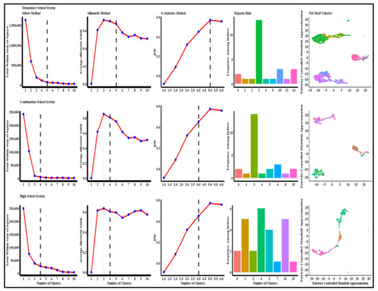
Figure 2.
Potential optimal numbers of clusters.
The majority rule in Figure 2 measures the appropriateness of clusters using various indices [138]. Most statistical techniques for the elementary school system support five optimal clusters that provide the best visualization results with few outliers and minimal overlaps. For the combination and high school systems, visualization and statistical measures proposed four optimal clusters for each school system. Notice the two outliers for the high school system. The elementary school system’s inflection points for the Elbow, Silhouette, and G-Statistics methods are at five clusters. Indices in the majority rule also identify five optimal clusters, likewise the PaCMAP visualization. For the combination school’s system, whereas the Elbow, Silhouette, majority rule, and PaCMAP methods propose four clusters, the first inflection point for the G-Statistics method is five. While the Elbow and Silhouette methods suggest four clusters, the G-Statistics methods suggest five, the majority rule proposes four and six clusters for the high schools’ system, and the PaCMAP identifies six clusters with two outliers.
The results of internal clustering validation measures (i.e., connectivity index, Dunn Index, and Silhouette width) based on the Gowers distance of the original data and PAM are in Figure 3. The optimum value of the connectivity index should be minimum; Silhouette should be maximum; likewise, the Dunn index. In Figure 3, the three measures suggest three, six, and four optimal clusters for the elementary school system. Analogous results from the three measures are four, six, or seven for the combination school system and four, six, or seven for the secondary school system. The results from the three measures are as expected due to heterogeneity in the data. In Figure 2, each index has limitations, especially for a large dataset with outliers, and the results rely heavily on properties intrinsic to the dataset [12,74]. However, the Silhouette width is a widely used index for internal clustering validation and determining the quality of clusters and the entire classification [139]. The index provides enough information about clustering quality for unlabeled data and, therefore, suggests more accurate results regarding optimal numbers of clusters existing in the dataset.
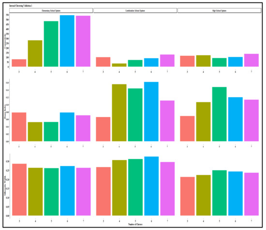
Figure 3.
Internal clustering validation measures.
To get the best and most consistent results, we use the Silhouette width results and modify the measure to determine the best-bet numbers of groups by comparing the weighted proportions of data points at the boundaries of each created cluster using the following formula (, where is the weighted negative Silhouette proportion, K is the number of clusters, , is the size of the cluster (number of observations in the cluster), n is the sample size (observations in the dataset), and is the number of data points with negative Silhouette width in each cluster. The weight can evaluate results produced by similar or different algorithms on equal or different numbers of clusters). The results from the proposed formula are such that the weighted ratio is zero for perfect partitioning and one for random data points with no visible groups.
The first panel of Figure 4 presents the reference points, suggested optimal clusters identified in Figure 2 and Figure 3, and potential optimal clusters using the proposed weighted formula for the elementary schools’ system; comparable results for the combination and high school systems are in Appendix B. In Figure 4, regarding the elementary schools’ system, the average Silhouette width and the weighted proportion for the width under three clusters were 0.26 and 0.129, compared to 0.26 and 0.093 for four clusters, 0.26 and 0.115 for five clusters, 0.27 and 0.041 for six clusters. In Figure 4, the elementary school system reference point is five clusters, and the results show that 11.5 percent of data points were on the boundaries compared to 12.9, 9.3, and 4.1 percent when portioned into three, four, and six, respectively. Notice that 13 and 39 percent of data points in clusters one and two under the four cluster assumptions were on the cluster boundaries. Analogous numbers are 2 (cluster 1), 17 (cluster 2), and 13 (cluster 4) under the six clusters assumption. Six clusters partition the elementary school’s system data better by positioning a few (per cluster) data points on the cluster’s boundaries. Moreover, the second panel of Figure 4 is the box plot of the average Silhouette of the referenced clusters. For the elementary school system, the results from six clusters show few outliers compared to the remaining clusters.
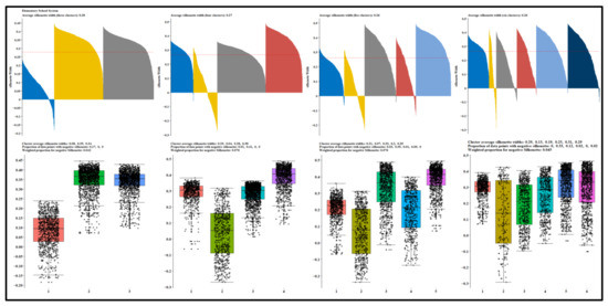
Figure 4.
Proportional data points on cluster boundaries and their distributions for the elementary school system.
The equivalent results for the combination and high school systems are in Appendix B. The weighted proportion for negative Silhouette width from the combination schools’ system suggests selecting among three, four, and seven clusters that indicate that 5.8, 6.0, and 6.4 percent of the data points were on boundaries. For six clusters, 12.8 percent of data points are on the borders. Partitioning the combination schools’ system into four groups produced better results. For example, 14 and 33 percent of clusters 1 and 3 are on boundaries compared to 7 and 25 data points in clusters 1 and 2 when the data is portioned into four clusters. The results for the high school system imply retaining seven groups that position only 5.3 percent of the data point on the boundaries of the created clusters, and only cluster one has 11 percent of the data points on the edge of the group. Also, the data points with a negative Silhouette are less than one percent among all seven clusters for the high school system.
Figure 5 presents the annotated clusters with school performance scores and ellipses created using the Khachiyan algorithm (Gács and Lovász, 1981); the distance between the centroid and the furthest point in the cluster defines the radius of the circle. In Figure 5, SPS is the cluster medoid regarding SPS. In Figure 5, the pairwise controlled manifold approximation preserves both inter-cluster (global structure) and intra-cluster distance (local structure) distances (data geometry), the position of each cluster determines relatedness between clusters, and the size and spread of each cluster are proportional to the variance of the group and cluster membership. Figure 5 shows four unique groups of school clusters under the elementary schools system, denoted as extremely at-risk schools (the medoid SPS is 50.0), high-at-risk schools (the medoid SPS is 54.70), at-risk schools (the medoid SPS is 58.4, and exceeds expectations (the medoid SPS is 106.5). The meet-expectation cluster has a medoid score of 79.7, intersecting with exceeds expectations cluster with a medoid score of 92.3. Specific features for intersecting clusters are similar or share comparable attributes. The intersections or overlaps imply that the data points on the boundaries of these clusters are closer to data points in the neighboring cluster than to data points in its cluster.
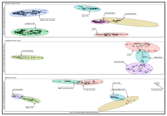
Figure 5.
School systems optimal clusters annotated with school performance scores.
Figure 5 also shows one unique cluster under the combination schools’ system; the remaining three are interrelated. The cluster with the failing schools had a medoid score of 48.0 and intersected with the at-risk Schools’ cluster with a medoid score of 59.3 and meets expectation schools with medoid scores of 89.9. The unique “exceed expectation schools cluster” had a medoid score of 120.8. For the high school system, one of the seven clusters is unique, that is, the needs improvement cluster with a medoid SPS of 79.6. This unique cluster contained two outliers; therefore, they were removed for further analysis. Three groups, each with two clusters, are interrelated. The first two interconnected clusters are extremely failing schools (the medoid SPS is 33.7) and lower- at-risk cluster (medoid SPS is 68.9). While the upper-at-risk Schools’ cluster interconnects with meet expectation clusters with the medoid SPS of 65.0 and 89.7, respectively, the exceeds expectation cluster (medoid SPS is 98.9) intersects with exceeds expectation cluster with a medoid of 101.3. The results in Figure 5 suggest that the organization of school performance in the State of Louisiana is not along a single dimension of indicators but meaningfully organized into heterogeneous clusters with unique and interconnected features.
4.2. Results from Supervised Learning Analyses
Reporting and comparing performance metrics is customary when evaluating machine learning models. Each metric has advantages and disadvantages; each reflects a different aspect of predictive performance. We used the holdout method to determine how statistical analysis can transform into a dataset, as explained in Section 2.2 and 2.3. The experimental part of the research covers the design of the test environment plus the formation of each model by splinting the datasets into training (80%) and validation (20%) sets. The algorithms used in this study include decision trees (DST), k-nearest neighbor (KKNN), stabilized linear discriminant analysis (SLDA), NSC (nearest shrunken centroids (NSC), penalized discriminant analysis (PDA), HDDA (high dimensional discriminant analysis (HDDA), random forest (RF), and gradient boosting machine (GBM). These are popular algorithms for multiclass classification. The summary statistics of each model’s performance metrics are in Table 2, and the relative distributions of the metrics are in Appendix C.
Table 2.
Metrics of machine learning models.
By comparing both “more-is-better” and “low-is-better” measures, the performance metrics in Table 2 results indicate that the random forest (RF) and gradient boosting machine (GBM) algorithms perform betters in predicting the created clusters for all school systems. More-is-better implies a preference for higher scores, and less-is-better means lower scores indicate better performance. Based on t-test results and more-is-better metrics, the RF and GBM models have the highest but similar scores with low standard deviations. The RF and GBM generated the best results related to the accuracy, kappa, recall, specificity, and detection rates (more-is-better) performance measures, with relatively small standard deviations compared to the results from other algorithms. The results imply that the RF and GBM results are more accurate and stable than other models. Also, the mean log losses for the RF and GBM are the lowest among all models. The mean log losses are statistically significantly lower for the GBM under the elementary and high school systems but higher for the combination school system. Therefore, we use the GBM results to identify features for the elementary and high school systems and RF results for the combination school system. Results in Table 2 show that the Decision Tree and K-nearest neighbor performed poorly across the three school systems. The emphasis of more-is-better performance measures is on avoiding “False Negative” or Type II errors. In statistics, type II errors mean failing to reject the null hypothesis when it is false. For RF and GBM, better measures are more than 0.95, implying that at least 95% of cluster members are in the ideal groups. A relatively higher detection rate suggests that the two algorithms are more likely to identify those members that do not belong in either cluster. In Table 2, the log-loss also focuses on model prediction performance. A model with perfect prediction has a log-loss score of 0; in other words, the model predicts each observation’s probability as the actual value. Therefore, the log-loss indicates how good or bad the prediction results are by denoting how far the predictions are from the actual values; thus, lower is better. Based on the results in Table 2, the RF and GBM models outperform all models for all school systems using more-is-better and low-is-better performance metrics.
For the elementary school system, we used the GBM models to identify critical features influencing school performance. Comparatively, in Table 2 (see also Appendix B), the mean and standard deviation estimates of the more-is-better performance metrics from the RF and GBM models are not statistically significantly different (p = 0.01) among the three Schools’ systems. However, while the mean values for the RF are consistently higher than those for the GBM models under the elementary school systems, the GBM model log-loss is lower (0.0448) and statistically different compared to the RF log-loss model (0.2268). Although not statistically significant, for the combination school system, the more-is-better metrics from the GBM are consistently higher and tighter (low standard deviation) compared to the RF results. Moreover, the mean Log-loss of the GBM model (0.1259) is statistically significantly lower (p = 0.01) than the mean log-loss for the RF model (0.3021). Therefore, the GBM is slightly better at predicting and classifying combination school system datasets than the RF model.
The performance metrics of the k-folds validation analysis are not statistically significant (p = 0.01) compared to the results from the training datasets. Similarly, Table 2 and Appendix C show that the RF’s more-is-better performance metrics are consistently higher but not statistically significantly different from the GBM model results. However, the mean logloss of the GBM (0.1485) is lower and statistically significant compared to the RF mean logloss (0.3651). Referring to these results, we also used GBM model results to identify the critical features of combination and high school systems. The estimated GBM best “metrics” using k-fold cross-validation were: accuracy (0.9927), kappa (0.9912), and logloss (0.012) for the elementary school system, accuracy (0.9876), kappa (0.9801), and logloss (0.023) for the combination school system and accuracy (0.9932), kappa (0.9911), and logloss (0.0165) for the high school system.
Generally, importance provides a score indicating how useful or valuable each feature was in constructing the boosted decision trees within the model. The more an attribute contributes to making critical decisions with decision trees, the higher its relative importance. Figure 6 shows the fifteen features (arbitrarily set) generated from the GBM (elementary and high school systems) and RF (combination schools system).
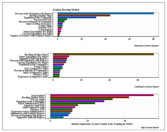
Figure 6.
Relative importance scores of variables at the school system levels.
In Figure 6, the critical features of the elementary school system are mainly related to community socioeconomic variables and school characteristics. The community variables (with the order of importance) include the percentage of the population with a bachelor’s degree (the dominant feature), dwelling median value, the total population in the community, the percentage of poverty in the community, and the relative number of minorities in the community. These variables are related to community affluence. The education literature always confirms a causal relationship between school performance and the socioeconomic status of communities. Socioeconomic status (SES) encompasses wealth, educational attainment, financial security, social status, and social class perception. Poverty is not a single factor but characterizes multiple physical and psychosocial stressors.
Further, SES is a consistent and reliable predictor of many life outcomes. Many studies (such as [140,141,142]) indicate that schools in low-SES communities perform poorly compared to schools in affluent neighborhoods, punctuated by the presence of minorities. Often, schools in low-SES communities have lower performance scores because students have poor cognitive development and lack language, memory, and socio-emotional processing. Consequently, their performance in schools is flawed. Moreover, the school systems in low-SES communities are often under-resourced, negatively affecting schools’ academic progress and outcomes, including inadequate education and increased dropout rates [128,143,144,145]. The State of Louisiana can reduce these risk factors through early intervention programs to improve the school systems with elevated identified critical features at the community level.
Solutions to improve the performance of Louisiana’s elementary school systems should focus on reducing teachers’ workload and boosting their morale through increased pay and other work-related incentives. The critical features related to school-level characteristics include the salary of other non-academic instructors, truancy rate, teachers’ full-time equivalent, total students in schools, salary expenditures and current expenditures per pupil, and the number of teachers with a graduate degree. These variables determine the workload, incentive, and morale of teachers and non-academic staff and the delivery of quality education to individual students. Frequently, schoolteacher and staff morale are associated with inequities from being overworked, lacking advancement, and low salaries resulting in unproductive school culture, which affects the administration, teaching, and learning [146,147]. Therefore, factors that cause low morale are from sources controllable by the school administrators and policymakers. Reducing teachers’ workload, class preparation time through smaller classrooms, administrative support, recognition, and opportunities for advancement offer administrators leverage to enhance or change the school culture.
The first four significant critical feature of the combination school system is the median dwelling values (the dominant feature), salary expenditure per pupil, support staff with a degree, and percentage of the population with a degree. Except for the experience of the support staff, although not in a similar order, other remaining variables appear as critical features in the elementary school’s system. Apart from community affluence and teachers’ and staff morale, the support staff experience was also an essential feature of the combination school system. Positive school culture thrives by including support staff and all non-teaching teams who play a crucial role in ensuring students learn in a safe and supportive learning environment. They can foster positive, trusting relationships with students and improve the school climate by encouraging parent and family involvement in their student’s education [148,149]. In Louisiana, schools rely on the professional input and expertise of a range of staff; some work alongside teachers, and some work behind the scenes to ensure an efficient infrastructure for effective teaching and learning. As the chief executive officers, the school principals should initiate a consistent, compelling reward system to motivate their job performance and general welfare. Often overlooked, legislators should ensure that the combination school system has a pool of efficient and motivated support staff to support learning in this diverse and complex school system.
The four dominant features of the high school system are total students (the most predominant), dwelling median value, the population in the community, and full-time equivalent per pupil. The second groups are variables related to workload (i.e., school administrator, support staff, and teacher FTE) and incentives (i.e., the salary of support staff). The remaining variables are allied to the experience and education of administrators and teachers (i.e., the experience of administrators, administrators with a graduate degree, and support staff with a degree) and a community-level variable (i.e., the percent of the population with a degree). Apart from community affluence, the experience and education of administrators and support staff were critical features within the high school systems. A successful school is about much more than teaching. While good teaching and learning are crucial, experienced administrators are vital in providing a well-rounded and effective teaching environment. Experienced administrators and support staff allow academic staff and teachers to focus on teaching. At the same time, they create robust systems for accountability, policies, and procedures to ensure that teaching and learning flow as smoothly as possible. An effective administration department can extract and analyze critical data to inform schools’ strategic decisions around education provision [150,151,152,153].
In addition, employee retention does not have a one-size-fits-all solution. Each school system and individual school must work purposefully to devise plans to retain its most influential administrators and teachers [149,154]. The State of Louisiana can reduce administrators turnover through beneficial job contracts, the tenure system, and a higher salary for administrators and teachers in the high school system. Additionally, creating a positive disciplinary environment lowers the odds of principals moving to another school, especially in high concentrations of students of color. Moreover, allowing the administrators to influence and determine teacher professional development and budgeting decrease the likelihood of principal turnovers.
The ladder/spider plots in Appendix D illustrate the most prominent features within each identified cluster in each school system relative to the average school system values. The plotted variables are scaled (range standardized from 0 to 1) and represent lacking (0) to abundant (1); therefore, the spokes radiate outwards from a central zero hub. The center of the wheel or the x-axis represents a minimum value, which is zero; the mid-cycle and the last cycles represent the average (0.5) and the maximum (1). The red color represents the cluster’s average values, and the green color is the school system’s average value. The denotation of the clusters is ordinal and consists of three groups: SPS below 60 (failing schools, extremely at risk, highly at risk, and at risk), the SPS between 60 and 80 (lower at risk and meet expectation), and SPS above 80 (exceed expectations and highly exceeds expectations). Therefore, six clusters exist for the elementary school system (the 7th cluster included only outliers), and four and six prominent groups exist for the combination and high school systems. School-level attributes that distinguished the school system cluster include truancy rate, availability of transportation services, teacher FTE per pupil, the average salary of other support staff, the average wage of administrators, and the number of support staff with undergraduate and number of instructors with graduate degrees. Community-level attributes were the percentage of the population with degrees, median dwelling values, population size, the portion of the people in poverty, and population median age.
The medoid SPS score for the elementary school system was 52.0 for the extremely at-risk cluster. The cluster’s truancy rate, transportation services, and salaries for administrators and instructors are below the elementary school system average; likewise, the number of support staff with graduate degrees. Also, the number of teachers and support staff with graduate degrees was below the average for elementary schools. Most of the schools in this cluster are in low-populated communities with a young population and below-average wealth, measured by dwelling value. The poverty rate (based on income) in these communities is relatively low, and the percentage of people with a degree is above average, which signals the characteristics of working-class communities. Parents in these communities (working class) drives their children to schools (low truancy rate) when going to work. Although the FTE per pupil is above average, working parents might not have enough time to support their students academically, such as helping them with homework and other assignments. To increase performance, instituting effective mentoring, tutoring, and after-school education programs that provide motivation, personal individual attention, direct instruction, and access to textbooks and instructional materials to increase schools’ academic skills and support services [155,156,157,158]. Increasing the number of experienced administrators, staff, and teachers through new hires would boost the performance of the schools in the cluster.
Although transportation service in the “high-at-risk” cluster (medoid SPS of 54.7) is average, there is an elevated truancy rate. In this cluster, the number of support staff with an undergraduate degree is deficient, and teacher FTE per pupil is below the average. Schools in the groups are in young, high-populated, and relatively affluent communities with low poverty rates, but the population with the degree is below average. Low teacher FTE per pupil might indicate instructor understaffing that limits the process of identifying students with specific instructional needs. Increasing the number of instructors and collaborating with parents to reduce truancy would improve school performance. There is a need for intervention programs that dispel parental misbeliefs undervaluing the importance of regular attendance and the number of school days their child misses classes [159,160]. Truancy reduction efforts need a differentiated approach that targets risk factors more prevalent in a specific group of students and tailored concerted efforts to ensure chronic absentee students can get back on track.
Except for the above-average numbers of instructors with an undergraduate degree and slightly higher teacher FTE per pupil, the at-risk cluster with medoid SPS of 58.4 is like the high-at-risk cluster discussed above. Schools in the cluster serve vulnerable populations facing educational and economic barriers [161]. Besides mentoring, tutoring, and after-school education programs, such schools need to be recognized and supported with more physical, human, and financial resources. An increase in teacher FTE per pupil indicates increased student support [162] with direct and positive effects on school performance. Although the values of most attributes are below average, the teacher FTE per pupil for the cluster that meets expectations (medoid SPS of 79.7) was above average. Except for the number of support staff with a graduate degree, dwelling median value, and population size, the two clusters that exceed expectation (medoid SPS of 92.3) and highly exceed expectation (medoid SPS of 106.5), all other variables are within the elementary school averages. The schools in these clusters are in communities with low populations, but the percentage of the people with a degree is above average, and the population’s median age is below average, implying that these schools are in large affluent communities with resources to support the school systems.
For the combination school system, schools in the “failing Schools” cluster where a medoid had an SPS of 48 are in large communities with medium wealth measured by median dwelling values. Although the number of instructors with a graduate degree is slightly above average, other schools’ and community-levels attributes are below the school system averages. Excluding the population percentage with the degree variable, all other characteristics for the “at-risk” cluster (medoid SPS of 59.3) were below the average, implying various interrelated variables influence Schools’ performances. For both clusters, improvement in leadership will churn the interwoven network [163], resulting in positive structural and administrative changes that improve school performance [164]. Some of the attributes of the “meet expectation” cluster (medoid of SPS of 89.9) were above the school system average. These variables include the number of instructors with a graduate degree, dwelling medium values, population size, and average salary of school administrators. In the extant education literature, these are critical factors influencing school performance. For the “exceeded expectation” cluster where the medoid had an SPS of 120.8, the percentage of the population with a graduate degree and the teacher FTE per student was above average, and the truancy rate was below the school system average.
After dropping the outliers, the high school system had six clusters. The SPS for the medoid of the “upper at risk” cluster was 58.4. The above-average attributes for the group were the percentage of the population in poverty, the number of support staff with a graduate degree, dwelling medium values, and population size. School-level and community-level attributes within the cluster that was below average included the number of support staff without a graduate degree and the percentage of the population with graduate degrees. The schools in the cluster were in densely populated communities with high poverty rates commonly associated with poor school performance. These schools need active instruction that increases student engagement, a critical element of academic achievement in schools with students from families in poverty and at risk for adverse outcomes [165]. For the “lower-at-risk” cluster where the SPS for the medoid was 66.9, the above-average attributes were percent of the population in poverty, percent of people in poverty, and teacher FTE per pupil. Schools in the cluster were in relatively less affluent small communities with high poverty rates. The truancy rate, the salary of administrators, and the number of support staff with an undergraduate degree were below the cluster average.
Solid administrative leadership is a critical component of schools with high student achievement. Students receive more individualized help, and attention from the support staff; teachers receive specialist support and assistance with their administrative and planning tasks, granting them more time for their core responsibilities [166]. The medoid of the “highly needs improvement” cluster had an SPS of 71.3. The attributes representing the number of support staff without a graduate degree, the number of support staff with a degree, and percent of the population with a degree were above average. The schools in this cluster were in moderately affluent and medium-sized communities with low poverty rates that differentiate it from the “upper-at-risk” and “lower-at-risk” clusters. The medoid of the “meet expectation” cluster had an SPS of 90.0, and the schools in the group were in moderately affluent, medium-sized communities and relatively above-average median age. The number of support staff with graduate degrees and the salary of administrators in these schools was above average, boosting the overall school performance.
The “exceeds expectation” cluster attributes (SPS of 102.2) are almost like the “highly needs improvement” cluster. They differ in two features: the percentage of the population with a degree and support staff without an undergraduate degree. The medoid of SPS, the “highly exceeds expectation cluster,” was 131.5. The schools were in moderately affluent and low-populated communities, with above-average percent females in the population and a percentage of people with a degree and support staff without an undergraduate degree. In the cluster, the above-average unique attribute is the percentage of females in the population. Education research has found that parents with high education significantly influence their children’s educational and career aspirations through increased parent involvement in student education activities [158]. Education studies (such as [157,167,168]) also report a strong correlation between single parents and reviewing student report cards, as well as attending field trips and school activities, with a positive effect on students’ performance.
5. Summary and Conclusions
There are three main categories in Louisiana public schools: elementary/middle school system (1–8 grade), combination school system (1–12 grade), and high school system (9–12 grade). These schools persistently perform below the national average. Louisiana public schools perform below the national average. The base of the analyses is the data from 2015/16, 2016/17, and 2017/18 school years data available from the Louisiana Department of Education Data Center. The data include school performance scores, student characteristics, and school attributes combined with community-level variables from the 2019 American Community Survey (ACS). The ACS provides data annually and covers a broad range of topics about the U.S. population’s social, economic, demographic, and housing characteristics.
The objectives were to group the schools into homogenous clusters and identify subgroups based on critical features influencing their performance. This study uses a pairwise controlled manifold approximation technique as a multidimensional reduction technique to visualize and create the base clusters. We also used gradient-boosting machine learning to characterize the homogenous clusters at the school system and subgroup levels. Results indicate that the elementary/middle school system is in six homogenous clusters, the combination school system is in four groupings, and the high school system is in six groups. Failing schools were generally in densely populated and low affluent communities, with high truancy rates, below average teacher FTE per pupil, administrators’ salaries, and the number of support staff. High-performing schools were in communities with a high percentage of the population with a graduate degree, moderately affluent and smaller communities, and administrators’ salaries and numbers of support staff were relatively high.
Our results indicate that investing resources to increase the number of support staff and hiring administrators with more experience (implying (higher pay) can be economically more effective than simply increasing the per-pupil spending, at least in the short term. To improve school performance, policymakers and administrators must first identify attributes of persistently struggling schools and engage the community in developing evidence-based plans to solve a specific problem. Funding for struggling schools must focus on the quality of every school, from the excellence of the instruction to the rigor of the classes and equal access to resources (such as adequate support staff) shown to be fundamental to quality education and school performance. However, re-evaluating the results is necessary when the post-COVID-19 pandemic data is available.
Author Contributions
A.R.K. collected and analyzed the data and wrote the first draft. D.R.A. compiled the literature and revised the final draft. All authors have read and agreed to the published version of the manuscript.
Funding
The U.S. Department of Commerce’s Economic Development Administration funded this study through the University Center for Economic Development at Southern University and A&M College, Baton Rouge, Louisiana, through award # 80-66-04881. However, the views expressed in this paper are those of the author and do not necessarily represent the view of the Economic Development Administration and Southern University and A&M College.
Institutional Review Board Statement
Not applicable.
Informed Consent Statement
Not applicable.
Data Availability Statement
Data is available online. Clean data are available on request.
Conflicts of Interest
The authors declare no conflict of interest.
Appendix A. Summary Statistics of the Covariate Variables
| Variables | 2015/16 | 2016/17 | 2017/18 | |||
| Average | Std.Dev | Average | Std.Dev | Average | Std.Dev | |
| Elementary schools system | ||||||
| School performance score | 82.94 | 20.33 | 79.96 | 21.28 | 70.41 | 15.46 |
| Salary expenditure per pupil ($) | 5322.00 | 1374.00 | 5421.00 | 1522.00 | 5518.00 | 1556.00 |
| Current expenditure per pupil ($) | 11,081.00 | 1435.00 | 11,259.00 | 1475.00 | 11,591.00 | 1593.00 |
| Full-time equivalent certified teachers | 32.13 | 12.87 | 32.37 | 13.1 | 32.34 | 13.32 |
| Full-time equivalent other instructors | 8.86 | 5.11 | 9.04 | 5.33 | 8.78 | 5.29 |
| Full-time equivalent support staff | 4.52 | 2.86 | 4.54 | 2.65 | 4.57 | 2.95 |
| Full time Equivalent administrative staff | 3.97 | 1.53 | 3.95 | 1.65 | 4 | 1.77 |
| Full-time Equivalent transportation services | 4.46 | 3.68 | 4.41 | 3.74 | 4.29 | 3.43 |
| Full-time equivalent other staff | 8.08 | 3.76 | 7.92 | 3.68 | 7.83 | 3.54 |
| Salary of certified teachers | 48,530.00 | 4079.00 | 49,036.00 | 3686.00 | 49,590.00 | 3978.00 |
| Salary of other teachers | 20,373.00 | 4112.00 | 20,539.00 | 4021.00 | 21,036.00 | 4248.00 |
| Salary of administrators | 49,408.00 | 8566.00 | 49,656.00 | 9607.00 | 50,632.00 | 9588.00 |
| Salary of support staff | 21,043.00 | 5625.00 | 21,214.00 | 5493.00 | 21,829.00 | 6074.00 |
| Number of support instructors without bachelor’s degree | 12.13 | 5.22 | 12.15 | 5.16 | 12.06 | 5.12 |
| Percentage of instructors without bachelor’s degree | 0.86 | 1.06 | 0.99 | 1.22 | 1.04 | 1.25 |
| Percent of administrators without bachelor’s degree | 2.93 | 1.36 | 2.88 | 1.4 | 2.87 | 1.33 |
| Percent of Support Staff without bachelor’s degree | 33.3 | 8.8 | 33.22 | 8.5 | 32.93 | 8.72 |
| Percent of certified teachers with bachelor’s degree | 37.77 | 8.7 | 37.58 | 8.48 | 37.8 | 8.54 |
| Percent non-instruction teacher with bachelor’s degree | 2.56 | 3.73 | 2.61 | 3.33 | 2.38 | 2.65 |
| Percentage of uncertified teachers without bachelor’s degree | 2.12 | 2.22 | 2.03 | 1.97 | 1.92 | 1.8 |
| The percentage of Support Staff with bachelor’s degree | 42.93 | 9.3 | 42.78 | 8.7 | 42.74 | 8.96 |
| The percentage of certified teachers with a graduate degree | 14.84 | 7 | 15.16 | 6.91 | 15.37 | 6.82 |
| Percent of uncertified instructors with a graduate degree | 4.43 | 2.22 | 4.36 | 2.21 | 4.39 | 2.16 |
| Percent of administrators with a graduate degree | 3.33 | 1.34 | 3.29 | 1.27 | 3.35 | 1.32 |
| Percent of support staff with a graduate degree | 22.7 | 7.62 | 22.92 | 7.59 | 23.2 | 7.58 |
| Percent of support staff with specialized training | 0.7 | 1.09 | 0.7 | 1.15 | 0.71 | 1.2 |
| Years of experience as a certified teacher | 12.48 | 3.23 | 12.56 | 3.18 | 12.46 | 3.24 |
| Years of experience of other support staff | 10.04 | 4.26 | 9.98 | 4.32 | 9.99 | 4.55 |
| Years of experience of uncertified teachers | 15.79 | 5.56 | 15.64 | 5.47 | 15.66 | 5.72 |
| Years of experience as administrators | 17 | 5.56 | 16.93 | 5.67 | 16.64 | 5.55 |
| Years of experience support staff | 12.26 | 2.48 | 12.31 | 2.46 | 12.21 | 2.56 |
| Percent student attendance | 93.57 | 8.17 | 93.03 | 8.45 | 93.79 | 5.33 |
| Percent of classes with 21–26 students | 35.15 | 20.64 | 33.29 | 20.93 | 33.05 | 20.64 |
| Percent of classes with 27–33 students | 9.07 | 11.42 | 8.86 | 11.32 | 8.8 | 11.06 |
| Percent of classes with more than 34 students | 2.7 | 3.44 | 2.14 | 2.1 | 2.43 | 3.2 |
| School expulsion rate | 0.48 | 0.92 | 0.44 | 0.7 | 0.47 | 0.81 |
| Percentage of students retained | 3.59 | 2.85 | 3.33 | 2.85 | 3.33 | 2.85 |
| Percent truancy | 28.9 | 13.91 | 33.67 | 14.96 | 49.36 | 16.11 |
| Total number of students | 486.7 | 205.1 | 481.8 | 219.1 | 489.2 | 215.6 |
| Percentage of female students | 47.77 | 5.31 | 47.51 | 6.39 | 48.39 | 3.24 |
| Percent of fully proficient students | 96.82 | 5.59 | 96.24 | 6.5 | 96.27 | 6.64 |
| Percent of students with limited English proficiency | 3.25 | 5.51 | 3.52 | 5.96 | 3.87 | 6.57 |
| Percent of minority students | 53.27 | 29.85 | 55.95 | 28.8 | 58.06 | 29.35 |
| The median age in the population | 36.49 | 2.39 | 36.42 | 2.32 | 36.44 | 2.41 |
| Size of the population | 170,995.00 | 140,173.00 | 169,249.00 | 138,958.00 | 171,784.00 | 140,807.00 |
| Dwelling median value | 139,167.00 | 38,976.00 | 138,039.00 | 38,840.00 | 138,188.00 | 37,209.00 |
| Percent of the population in poverty | 3.6 | 1 | 3.69 | 0.97 | 3.75 | 0.96 |
| Percent of the population with a degree | 86.04 | 5.3 | 86.07 | 5.33 | 86.01 | 5.25 |
| Combination schools system | ||||||
| School Performance Score | 87.45 | 23.25 | 88.75 | 22.35 | 78.51 | 19.11 |
| Salary expenditure per pupil ($) | 5887.00 | 2503.00 | 6027.00 | 3083.00 | 6051.00 | 2860.00 |
| Current expenditure per pupil ($) | 12,043.00 | 6220.00 | 12,529.00 | 8736.00 | 12,014.00 | 2748.00 |
| Full-time equivalent certified teachers | 34.77 | 18.1 | 35.03 | 18.81 | 34.31 | 16.48 |
| Full-time equivalent other instructors | 6.68 | 4.66 | 6.53 | 4.7 | 6.52 | 4.56 |
| Full-time equivalent support staff | 4 | 3.14 | 4.32 | 3.85 | 4.05 | 3.27 |
| Full-time equivalent administrative staff | 4.53 | 2.45 | 4.6 | 2.4 | 4.56 | 2.55 |
| Full-time equivalent transportation services | 5.63 | 3.41 | 5.44 | 3.35 | 5.37 | 3.33 |
| Full-time equivalent other staff | 8.87 | 4.41 | 8.74 | 4.21 | 8.29 | 4.02 |
| Salary of certified teachers | 49,649.00 | 4694.00 | 49,790.00 | 4349.00 | 50,341.00 | 5140.00 |
| Salary of other teachers | 21,756.00 | 6325.00 | 21,925.00 | 6418.00 | 21,297.00 | 6499.00 |
| Salary of administrators | 47,902.00 | 11,992.00 | 49,319.00 | 9795.00 | 50,047.00 | 12,726.00 |
| Salary of support staff | 22,032.00 | 9419.00 | 22,707.00 | 10,844.00 | 22,311.00 | 9420.00 |
| Number of support instructors without bachelor’s degree | 9.03 | 5.15 | 8.74 | 5.6 | 9.11 | 5.24 |
| Percentage of instructors without bachelor’s degree | 0.97 | 1.53 | 1.03 | 1.44 | 1.12 | 1.61 |
| Percent of administrators without bachelor’s degree | 3.11 | 1.37 | 3.27 | 1.43 | 3.31 | 2.1 |
| Percent of Support Staff without bachelor’s degree | 34.17 | 10.61 | 33.69 | 9.53 | 33.91 | 10.15 |
| Percent of certified teachers with bachelor’s degree | 36.54 | 8.94 | 36.32 | 8.65 | 36.94 | 8.58 |
| Percent non-instructional teachers with bachelor’s degree | 1.78 | 2.98 | 1.79 | 3.41 | 1.56 | 2.45 |
| Percentage of uncertified teachers without bachelor’s degree | 1.91 | 1.68 | 2.03 | 1.81 | 2 | 1.82 |
| Percent of Support Staff with bachelor’s degree | 40.44 | 8.62 | 40.67 | 7.79 | 40.63 | 8.86 |
| The percentage of certified teachers with a graduate degree | 17.35 | 11.1 | 17.06 | 7.99 | 16.94 | 8.44 |
| Percent of uncertified instructors with a graduate degree | 3.49 | 2.22 | 3.5 | 2.05 | 3.47 | 1.96 |
| Percent of administrators with a graduate degree | 3.46 | 1.35 | 3.57 | 1.37 | 3.73 | 1.7 |
| Percent of support staff with a graduate degree | 24.46 | 11.52 | 24.43 | 9.43 | 24.3 | 9.86 |
| Percent of support staff with specialized training | 0.62 | 0.98 | 0.69 | 1.11 | 0.83 | 1.71 |
| Years of experience as a certified teacher | 13.61 | 3.32 | 13.68 | 3.2 | 13.92 | 3.87 |
| Years of experience of other support staff | 10.64 | 4.65 | 11.06 | 4.66 | 10.74 | 4.62 |
| Years of experience of uncertified teachers | 15.94 | 7.04 | 16.27 | 7.03 | 17.02 | 7.49 |
| Years of experience as administrators | 17.1 | 4.85 | 16.34 | 5.21 | 17.21 | 5.28 |
| Years of experience of support staff | 13.1 | 2.78 | 13.07 | 2.46 | 13.44 | 2.84 |
| Percent student attendance | 92.42 | 7.83 | 91.78 | 8.12 | 93.08 | 2.94 |
| Percent of classes with 21–26 students | 15.63 | 10.64 | 16.53 | 11.26 | 16.73 | 10.87 |
| Percent of classes with 27–33 students | 7.82 | 8.24 | 7.4 | 7.98 | 7.87 | 9.35 |
| Percent of classes with more than 34 students | 2.07 | 2.72 | 2.06 | 4.79 | 2.49 | 5.41 |
| School expulsion rate | 0.64 | 1.15 | 0.67 | 1.47 | 0.7 | 1.66 |
| Percentage of students retained | 5.27 | 8.15 | 4.21 | 6.78 | 3.85 | 5.1 |
| Percent truancy | 26.96 | 14.97 | 33.73 | 17 | 53.69 | 16.63 |
| Total number of students | 499.2 | 285.8 | 525.3 | 351.1 | 510.4 | 326 |
| Percentage of female students | 46.67 | 8.34 | 47.17 | 7.1 | 47.52 | 6.51 |
| Percent of fully proficient students | 98.09 | 11.09 | 98.78 | 6.56 | 99.21 | 1.33 |
| Percent of students with limited English proficiency | 0.91 | 0.97 | 0.99 | 1.07 | 1.08 | 1.2 |
| Percent of minority students | 40.39 | 30.53 | 40.95 | 29.53 | 41.19 | 29.64 |
| The median age in the population | 37.47 | 3.32 | 37.49 | 3.25 | 37.54 | 3.26 |
| Size of the population | 89,843.00 | 115,074.00 | 84,773.00 | 115,033.00 | 79,577.00 | 110,879.00 |
| Dwelling median value | 113,667.00 | 35,055.00 | 110,891.00 | 32,344.00 | 108,294.00 | 31,221.00 |
| Percent of the population in poverty | 4.05 | 1.1 | 4.12 | 1.03 | 4.21 | 1.06 |
| Percent of the population with a degree | 88.93 | 4.1 | 89.36 | 4.03 | 89.33 | 3.8 |
| High schools system | ||||||
| School performance score | 89.65 | 20.68 | 90.17 | 23.64 | 80.29 | 21.14 |
| Salary expenditure per pupil ($) | 5423.00 | 1961.00 | 5595.00 | 2146.00 | 5737.00 | 2376.00 |
| Current expenditure per pupil ($) | 11,321.00 | 2540.00 | 11,557.00 | 2510.00 | 12,018.00 | 2724.00 |
| Full-time equivalent certified teachers | 53.4 | 29.58 | 54.24 | 31.22 | 56.04 | 30.33 |
| Full-time equivalent other instructors | 9.28 | 8.09 | 9.05 | 8.11 | 8.56 | 5.94 |
| Full-time Equivalent Support Staff | 6.84 | 4.52 | 6.91 | 4.33 | 7.03 | 4.65 |
| Full-time equivalent administrative staff | 7 | 3.5 | 6.96 | 3.53 | 7.21 | 3.7 |
| Full-time equivalent transportation services | 6.25 | 7 | 6.08 | 6.32 | 5.91 | 6.52 |
| Full-time equivalent other staff | 12.42 | 6.33 | 11.97 | 6.33 | 12.15 | 6.12 |
| Salary of certified teachers | 50,847.00 | 4171.00 | 51,111.00 | 3757.00 | 51,634.00 | 4203.00 |
| Salary of other teachers | 23,277.00 | 8017.00 | 24,138.00 | 11,237.00 | 24,273.00 | 9258.00 |
| Salary of administrators | 50,680.00 | 10,211.00 | 52,632.00 | 9440.00 | 54,377.00 | 11,818.00 |
| Salary of support staff | 21,891.00 | 8351.00 | 22,893.00 | 9232.00 | 22,990.00 | 7072.00 |
| Number of support instructors without bachelor’s degree | 6.62 | 3.3 | 6.83 | 3.39 | 6.9 | 3.09 |
| Percentage of instructors without bachelor’s degree | 1.08 | 1.25 | 1.08 | 1.2 | 1.09 | 1.19 |
| Percent of administrators without bachelor’s degree | 3.39 | 1.65 | 3.31 | 1.8 | 3.25 | 1.75 |
| Percent of Support Staff without bachelor’s degree | 29.24 | 9.57 | 29.05 | 10.1 | 28.62 | 9.95 |
| Percent of certified teachers with bachelor’s degree | 34.25 | 9.01 | 33.9 | 9.72 | 35.3 | 8.02 |
| Percent noninstructional teacher with a bachelor’s degree | 3.79 | 7.85 | 3.43 | 7.25 | 2.35 | 3.1 |
| Percentage of uncertified teachers without bachelor’s degree | 1.87 | 2.03 | 1.93 | 2.12 | 1.72 | 2.11 |
| Percent of Support Staff with bachelor’s degree | 40.27 | 8.76 | 39.93 | 9.16 | 40.15 | 9.16 |
| Percentage of certified teachers with a graduate degree | 20.16 | 7.19 | 20.43 | 7.91 | 20.46 | 7.59 |
| Percent of uncertified instructors with a graduate degree | 4.35 | 2.11 | 4.43 | 2.08 | 4.66 | 2.29 |
| Percent of administrators with a graduate degree | 3.55 | 1.37 | 3.51 | 1.41 | 3.73 | 1.47 |
| Percent of support staff with a graduate degree | 28.72 | 7.39 | 29.19 | 8.13 | 29.25 | 8.3 |
| Percent of support staff with specialized training | 0.6 | 0.83 | 0.63 | 0.9 | 0.61 | 0.88 |
| Years of experience as a certified teacher | 13.08 | 3.35 | 12.79 | 3.6 | 12.62 | 3.45 |
| Years of experience of other support staff | 10.28 | 4.01 | 10.61 | 4.72 | 10.66 | 5.04 |
| Years of experience of uncertified teachers | 17.06 | 5.7 | 16.65 | 6.03 | 16.45 | 6.02 |
| Years of experience as administrators | 17.56 | 5.44 | 17.17 | 5.33 | 16.76 | 5.29 |
| Years of experience support staff | 12.85 | 2.82 | 12.71 | 2.99 | 12.58 | 2.93 |
| Percent student attendance | 91.49 | 7.24 | 89.68 | 10.17 | 91 | 5.97 |
| Percent of classes with 21–26 students | 19.46 | 7.7 | 19.85 | 8.69 | 19.47 | 7.79 |
| Percent of classes with 27–33 students | 14.29 | 9.6 | 13.04 | 9.7 | 13.44 | 9.15 |
| Percent of classes with more than 34 students | 4.52 | 8.58 | 3 | 4.09 | 2.52 | 3.31 |
| School expulsion rate | 0.94 | 1.1 | 0.88 | 1.07 | 1.05 | 1.34 |
| Percentage of students retained | 6.62 | 8.08 | 6.09 | 8.46 | 5.93 | 8.93 |
| Percent truancy | 34.71 | 18.3 | 40.44 | 21.29 | 57.32 | 20.97 |
| Total number of students | 868.4 | 516.5 | 862.8 | 532.5 | 878 | 524 |
| Percentage of female students | 49.48 | 6.7 | 49.15 | 5.55 | 49.35 | 4.85 |
| Percent of fully proficient students | 97.33 | 7.72 | 97.84 | 4.24 | 97.45 | 4.69 |
| Percent of students with limited English proficiency | 2.04 | 3.79 | 2.2 | 4.2 | 2.69 | 4.63 |
| Percent of minority students | 53.55 | 28.77 | 56.65 | 27.51 | 59.15 | 28.53 |
| The median age in the population | 36.58 | 2.34 | 36.39 | 2.22 | 36.4 | 2.29 |
| Size of the population | 175,890.00 | 150,065.00 | 186,035.00 | 152,461.00 | 184,862.00 | 150,594.00 |
| Dwelling median value | 136,150.00 | 40,501.00 | 138,381.00 | 41,289.00 | 137,832.00 | 39,231.00 |
| Percent of the population in poverty | 3.74 | 1.12 | 3.82 | 1.01 | 3.87 | 1.02 |
| Percent of the population with a degree | 86.14 | 5.41 | 85.54 | 5.77 | 85.63 | 5.56 |
Appendix B. Proportion Data Points on Cluster Boundaries and Their Distributions for the Combination and High Schools Systems


Figure A1.
Distribution of data points on cluster boundaries.
Figure A1.
Distribution of data points on cluster boundaries.


Appendix C. Distribution of Performance Metrics of the Machine Learning Models

Figure A2.
Performance metrics for the elementary schools’ system.
Figure A2.
Performance metrics for the elementary schools’ system.


Figure A3.
Performance metrics for the combination schools’ system.
Figure A3.
Performance metrics for the combination schools’ system.


Figure A4.
Performance metrics for the high schools’ system.
Figure A4.
Performance metrics for the high schools’ system.

Appendix D. Important Features at the School Level

Figure A5.
Important features of the elementary schools’ system (extremely and high at risk).
Figure A5.
Important features of the elementary schools’ system (extremely and high at risk).


Figure A6.
Important features of the elementary schools’ system (at-risk and need improvement).
Figure A6.
Important features of the elementary schools’ system (at-risk and need improvement).


Figure A7.
Important features of the elementary schools’ system (exceeds expectation and highly exceeds expectation).
Figure A7.
Important features of the elementary schools’ system (exceeds expectation and highly exceeds expectation).


Figure A8.
Important features of the combination schools’ system (failing schools and at-risk).
Figure A8.
Important features of the combination schools’ system (failing schools and at-risk).


Figure A9.
Important features of the combination schools’ system (meet the expectation and exceeds expectation).
Figure A9.
Important features of the combination schools’ system (meet the expectation and exceeds expectation).


Figure A10.
Important features of the high schools’ system (extremely and lower at-risk schools).
Figure A10.
Important features of the high schools’ system (extremely and lower at-risk schools).


Figure A11.
Important features of the high schools’ system (higher-at-risk and meet-expectation schools).
Figure A11.
Important features of the high schools’ system (higher-at-risk and meet-expectation schools).


Figure A12.
Important features of the high schools’ system (exceeds and highly-exceed-expectationschools).
Figure A12.
Important features of the high schools’ system (exceeds and highly-exceed-expectationschools).

References
- Kaufman, I.; Rousseeuw, P.J. Finding Groups in Data an Introduction to Cluster Analysis; John Wiley & Sons: Hoboken, NY, USA, 1990. [Google Scholar]
- Stanard, R.P. High school graduation rates in the United States: Implications for the counseling profession. J. Couns. Dev. 2003, 81, 217–221. [Google Scholar] [CrossRef]
- Rumberger, R.W. High school dropouts in the United States. In School Dropout and Completion: International Comparative Studies in Theory and Policy; Springer: Dordrecht, The Netherlands, 2011; pp. 275–294. [Google Scholar]
- Kirst, M.; Myburg, A.A.; De León, J.P.; Kirst, M.E.; Scott, J.; Sederoff, R. Coordinated genetic regulation of growth and lignin revealed by quantitative trait locus analysis of cDNA microarray data in an interspecific backcross of eucalyptus. Plant Physiol. 2004, 135, 2368–2378. [Google Scholar] [CrossRef] [PubMed]
- Christle, C.A.; Jolivette, K.; Nelson, C.M. School characteristics related to high school dropout rates. Remedial Spec. Educ. 2007, 28, 325–339. [Google Scholar] [CrossRef]
- World Economic Forum Report. The Future of Jobs Reports, World Economic Forum, Geneva. 2020. Available online: https://www.weforum.org/reports/the-future-of-jobs-report-2020 (accessed on 17 October 2022).
- Ho, A.D.; Lewis, D.M.; MacGregor Farris, J.L. The dependence on the growth-model results in proficiency cut scores. Educ. Meas. Issues Pract. 2009, 28, 15–26. [Google Scholar] [CrossRef]
- Yeagley, R. Separating Growth from Value Added. Sch. Adm. 2007, 64, 18. [Google Scholar]
- McCaffrey, D.F.; Lockwood, J.R.; Koretz, D.; Louis, T.A.; Hamilton, L. Models for value-added modeling of teacher effects. J. Educ. Behav. Stat. 2004, 29, 67–101. [Google Scholar] [CrossRef]
- Ryser, G.R.; Rambo-Hernandez, K.E. Using growth models to measure school performance: Implications for gifted learners. Gift. Child Today 2014, 37, 17–23. [Google Scholar] [CrossRef]
- Wang, Y.; Huang, H.; Rudin, C.; Shaposhnik, Y. Understanding how dimension reduction tools work: An empirical approach to deciphering t-SNE, UMAP, TriMap, and PaCMAP. J. Mach. Learn. Res. 2021, 22, 1–73. [Google Scholar]
- Liu, Y.; Li, Z.; Xiong, H.; Gao, X.; Wu, J. Understanding of internal clustering validation measures. In Proceedings of the 2010 IEEE International Conference on Data Mining, Sydney, Australia, 13–17 December 2010; IEEE: New York, NY, USA, 2010; pp. 911–916. [Google Scholar]
- Aly, M. Survey on multiclass classification methods. Neural Netw. 2005, 19, 1–9. [Google Scholar]
- Gentleman, R.; Carey, V.J. Unsupervised machine learning. In Bioconductor Case Studies; Springer: New York, NY, USA, 2008; pp. 137–157. [Google Scholar]
- Olden, J.D.; Joy, M.K.; Death, R.G. An accurate comparison of methods for quantifying variable importance in artificial neural networks using simulated data. Ecol. Model. 2004, 178, 389–397. [Google Scholar] [CrossRef]
- Bae, E.; Bailey, J.; Dong, G. A clustering comparison measure using density profiles and its application to discovering alternate clusterings. Data Min. Knowl. Discov. 2010, 21, 427–471. [Google Scholar] [CrossRef]
- Ferraro, M.B.; Giordani, P.; Serafini, A. fclust: An R Package for Fuzzy Clustering. R J. 2019, 11, 198. [Google Scholar] [CrossRef]
- Van der Maaten, L.; Hinton, G. Visualizing data using t-sne. J. Mach. Learn. Res. 2008, 9, 2579–2605. [Google Scholar]
- Van der Maaten, L.; Weinberger, K. Stochastic triplet embedding. In Proceedings of the 2012 IEEE International Workshop on Machine Learning for Signal Processing, Santander, Spain, 23–26 September 2012; IEEE: New York, NY, USA, 2012; pp. 1–6. [Google Scholar]
- McInnes, L.; Healy, J.; Melville, J. Umap: Uniform manifold approximation and projection for dimension reduction. arXiv 2018, arXiv:1802.03426. [Google Scholar]
- Amid, E.; Warmuth, M.K. A more globally accurate dimensionality reduction method using triplets. arXiv 2018, arXiv:1803.00854. [Google Scholar]
- Becht, E.; McInnes, L.; Healy, J.; Dutertre, C.-A.; Kwok, I.W.H.; Ng, L.G.; Ginhoux, F.; Newell, E.W. Dimensionality reduction for visualizing single-cell data using UMAP. Nat. Biotechnol. 2019, 37, 38–44. [Google Scholar] [CrossRef]
- Lawson, R.G.; Jurs, P.C. New index for clustering tendency and its application to chemical problems. J. Chem. Inf. Comput. Sci. 1990, 30, 36–41. [Google Scholar] [CrossRef]
- Handl, J.; Knowles, K.; Kell, D. Computational cluster validation in post-genomic data analysis. Bioinformatics 2005, 21, 3201–3212. [Google Scholar] [CrossRef]
- Liu, Y.; Li, Z.; Xiong, H.; Gao, X.; Wu, J.; Wu, S. Understanding and enhancement of internal clustering validation measures. IEEE Trans. Cybern. 2013, 43, 982–994. [Google Scholar]
- Louisiana Department of Education. Bulletin 111: The Louisiana School, District, and State Accountability. 2008. Available online: http://www.doa.louisiana.gov/osr/lac/28v83/28v83.doc (accessed on 17 October 2022).
- Louisiana Department of Education. Accountability. 2009. Available online: http://www.doe.state.la.us/lde/portals/accountabilitv.html (accessed on 17 October 2022).
- Louisiana Department of Education. School Performance Scores and School Profiles. 2021. Available online: https://www.louisianabelieves.com/docs/default-source/accountability/2019-2020-sps-updates.pdf?sfvrsn=7eab6618_2 (accessed on 17 October 2022).
- Adelson, J.L.; Dickinson, E.R.; Cunningham, B.C. A multigrade, multiyear statewide examination of reading achievement: Examining variability between districts, schools, and students. Educ. Res. 2016, 45, 258–262. [Google Scholar] [CrossRef]
- Nejatian, S.; Parvin, H.; Faraji, E. Using sub-sampling and ensemble clustering techniques to improve the performance of imbalanced classification. Neurocomputing 2018, 276, 55–66. [Google Scholar] [CrossRef]
- Agrawal, R.; Gehrke, J.; Gunopulos, D.; Raghavan, P. Automatic subspace clustering of high dimensional data. Data Min. Knowl. Discov. 2005, 11, 5–33. [Google Scholar] [CrossRef]
- Molchanov, V.; Linsen, L. Overcoming the curse of dimensionality when clustering multivariate volume data. In Proceedings of the VISIGRAPP (3: IVAPP), Funchal, Maderia, Portugal, 27–29 January 2018; pp. 29–39. [Google Scholar]
- Lloyd, S.P. Last square quantization in PCM. Bell Teleph. Lab. Pap. 1982, 28, 129–137. [Google Scholar]
- MacQueen, J. Classification and analysis of multivariate observations. In Proceedings of the 5th Berkeley Symposium on Mathematical Statistics and Probability, Berkeley, CA, USA, 21 June–18 July 1965 and 27 December 1965–January 7 1966; Volume 1: Statistics, pp. 281–297. [Google Scholar]
- Ruspini, E.H. Numerical methods for fuzzy clustering. Inf. Sci. 1970, 2, 319–350. [Google Scholar] [CrossRef]
- Duja, S.B.U.; Niu, B.; Ahmed, B.; Umar, M.; Amjad, M.; Ali, U.; Ur, Z.; Hussain, W. A proposed method to solve cold start problem using fuzzy user-based clustering. Int. J. Adv. Comput. Sci. Appl. 2020, 11, 529–536. [Google Scholar] [CrossRef]
- Bezdek, J.C. Cluster validity with fuzzy sets. J. Cybern. 1974, 3, 58–73. [Google Scholar] [CrossRef]
- Dunn, J.C. Well-separated clusters and optimal fuzzy partitions. J. Cybern. 1974, 4, 95–104. [Google Scholar]
- Mojarad, M.; Nejatian, S.; Parvin, H.; Mohammadpoor, M. A fuzzy clustering ensemble based on cluster clustering and iterative Fusion of base clusters. Appl. Intell. 2019, 49, 2567–2581. [Google Scholar] [CrossRef]
- Xue, M.; Zhou, L.; Kojima, N.; Dos Muchangos, L.S.; Machimura, T.; Tokai, A. Application of fuzzy c-means clustering to PRTR chemicals uncovering their release and toxicity characteristics. Sci. Total Environ. 2018, 622, 861–868. [Google Scholar] [CrossRef]
- Wang, H.; Fei, B. A modified fuzzy C-means classification method using a multiscale diffusion filtering scheme. Med. Image Anal. 2009, 13, 193–202. [Google Scholar] [CrossRef]
- Bahght, S.F.; Aljahdali, S.; Zanaty, E.A.; Ghiduk, A.S.; Afifi, A. A new validity index for fuzzy C-means for automatic medical image clustering. Int. J. Comput. Appl. 2012, 38, 1–8. [Google Scholar]
- Chao, R.J.; Chen, Y.H. Evaluation of the criteria and effectiveness of distance e-learning with consistent fuzzy preference relations. Expert Syst. Appl. 2009, 36, 10657–10662. [Google Scholar] [CrossRef]
- Chang, T.Y.; Chen, Y.T. Cooperative learning in E-learning: A peer assessment of student-centered using consistent fuzzy preference. Expert Syst. Appl. 2009, 36, 8342–8349. [Google Scholar] [CrossRef]
- Daniel, E.; Hofmann-Towfigh, N.; Knafo, A. School values across three cultures: A typology and interrelations. SAGE Open 2013, 3, 2158244013482469. [Google Scholar] [CrossRef]
- Sabitha, A.S.; Mehrotra, D.; Bansal, A. Delivery of learning knowledge objects using fuzzy clustering. Educ. Inf. Technol. 2016, 21, 1329–1349. [Google Scholar] [CrossRef]
- Hogo, M.A. Evaluation of e-learning systems based on fuzzy clustering models and statistical tools. Expert Syst. Appl. 2010, 37, 6891–6903. [Google Scholar] [CrossRef]
- Pechenizkiy, M.; Calders, T.; Vasilyeva, E.; De Bra, P. Mining the student assessment data: Lessons drawn from a small scale case study. In Proceedings of the Educational Data Mining 2008, The 1st International Conference on Educational Data Mining, Montreal, QC, Canada, 20–21 June 2008. [Google Scholar]
- Kabakchieva, D. Student performance prediction by using data mining classification algorithms. Int. J. Comput. Sci. Manag. Res. 2012, 1, 686–690. [Google Scholar]
- Yadav, R.S.; Singh, V.P. Modeling academic performance evaluation using fuzzy c-means clustering techniques. Int. J. Comput. Appl. 2012, 60, 16–23. [Google Scholar]
- Unlu, A.; Schurig, M. Computational Typologies of Multidimensional End-of-Primary-School Performance Profiles from an Educational Perspective of Large-Scale TIMSS and PIRLS Surveys. Curr. Issues Comp. Educ. 2015, 18, 6–25. [Google Scholar]
- Askari, S. Fuzzy C-Means clustering algorithm for data with unequal cluster sizes and contaminated with noise and outliers: Review and development. Expert Syst. Appl. 2021, 165, 113856. [Google Scholar] [CrossRef]
- Hinton, G.E.; Roweis, S. Stochastic neighbor embedding. In Advances in Neural Information Processing Systems 15, Proceedings of the Neural Information Processing Systems (NIPS 2002), Vancouver, BC, Canada, 9–14 December 2002; The MIT Press: Cambridge, MA, USA, 2002; pp. 15857–15864. [Google Scholar]
- Van Der Maaten, L. Accelerating t-SNE using tree-based algorithms. J. Mach. Learn. Res. 2014, 15, 3221–3245. [Google Scholar]
- Du, X.; Yang, J.; Hung, J.L. An Integrated Framework Based on Latent Variational Autoencoder for Providing Early Warning of At-Risk Students. IEEE Access 2020, 8, 10110–10122. [Google Scholar] [CrossRef]
- Baron, T.; Grossman, R.I.; Abramson, S.B.; Pusic, M.V.; Rivera, R.; Triola, M.M.; Yanai, I. Signatures of medical student applicants and academic success. PLoS ONE 2020, 15, e0227108. [Google Scholar] [CrossRef]
- Asim, M.; Shamshad, F.; Awais, M.; Ahmed, A. Introducing Data mining for Predicting trends in School Education of Pakistan: Preliminary results and future directions. In Proceedings of the Ninth International Conference on Information and Communication Technologies and Development, Lahore, Pakistan, 16–19 November 2017; pp. 1–5. [Google Scholar]
- Czibula, G.; Ciubotariu, G.; Maier, M.I.; Lisei, H. IntelliDaM: A Machine Learning-Based Framework for Enhancing the Performance of Decision-Making Processes. A Case Study for Educational Data Mining. IEEE Access 2022, 10, 80651–80666. [Google Scholar]
- Linderman, G.C.; Steinerberger, S. Clustering with t-SNE, provably. SIAM J. Math. Data Sci. 2019, 1, 313–332. [Google Scholar] [CrossRef]
- Linderman, G.C.; Rachh, M.; Hoskins, J.G.; Steinerberger, S.; Kluger, Y. Fast interpolation-based t-SNE for improved visualization of single-cell RNA-seq data. Nat. Methods 2019, 16, 243–245. [Google Scholar] [CrossRef]
- Bolukbasi, T.; Pearce, A.; Yuan, A.; Coenen, A.; Reif, E.; Viégas, F.; Wattenberg, M. An interpretability illusion for bert. arXiv 2021, arXiv:2104.07143. [Google Scholar] [CrossRef]
- Nolet, C.J.; Lafargue, V.; Raff, E.; Nanditale, T.; Oates, T.; Zedlewski, J.; Patterson, J. Bringing UMAP closer to the speed of light with GPU acceleration. In Proceedings of the AAAI Conference on Artificial Intelligence, Virtual, 2–9 February 2021; Volume 35, pp. 418–426. [Google Scholar]
- Amid, E.; Warmuth, M.K. TriMap: Large-scale dimensionality reduction using triplets. arXiv 2019, arXiv:1910.00204. [Google Scholar] [CrossRef]
- Kiefer, A.; Rahman, M. An Analytical Survey on Recent Trends in High Dimensional Data Visualization. arXiv 2021, arXiv:2107.01887. [Google Scholar] [CrossRef]
- Huang, H.; Wang, Y.; Rudin, C.; Browne, E.P. Towards a comprehensive evaluation of dimension reduction methods for transcriptomic data visualization. Commun. Biol. 2022, 5, 1–11. [Google Scholar] [CrossRef]
- Hu, Y.; Hathaway, R.J. An algorithm for clustering tendency assessment. WSEAS Trans. Math. 2008, 7, 441–450. [Google Scholar]
- Yuan, C.; Yang, H. Research on the K-value selection method of the K-means clustering algorithm. R J. 2019, 2, 226–235. [Google Scholar] [CrossRef]
- Rousseeuw, P.J. Silhouettes: A graphical aid to the interpretation and validation of cluster analysis. J. Comput. Appl. Math. 1987, 20, 53–65. [Google Scholar] [CrossRef]
- Kassambara, A.; Mundt, F. Package Factoextra. Extract and Visualize the Results of Multivariate Data Analyses: R Package Version 1.0.7; Foundation for Statistical Computing: Vienna, Austria, 2017. [Google Scholar]
- Charrad, M.; Ghazzali, N.; Boiteau, V.; Niknafs, A. NbClust: An R package for determining the relevant number of clusters in a data set. J. Stat. Softw. 2014, 61, 1–36. [Google Scholar] [CrossRef]
- Maulik, U.; Bandyopadhyay, S. Performance evaluation of some clustering algorithms and validity indices. IEEE Trans. Pattern Anal. Mach. Intell. 2002, 24, 1650–1654. [Google Scholar] [CrossRef]
- Tasdemir, K.; Merényi, E. A validity index for prototype-based clustering of data sets with complex cluster structures. IEEE Trans. Syst. Man Cybern. Part B (Cybern.) 2011, 41, 1039–1053. [Google Scholar] [CrossRef]
- Kim, Y.I.; Kim, D.W.; Lee, D.; Lee, K.H. A cluster validation index for GK cluster analysis based on the relative degree of sharing. Inf. Sci. 2004, 168, 225–242. [Google Scholar] [CrossRef]
- Van, C.T.; Blockeel, H. Using internal validity measures to compare clustering algorithms. In Proceedings of the Benelearn 2015 Poster Presentations, Online, 19 June 2015; pp. 1–8. [Google Scholar]
- Tibshirani, R.; Hastie, T.; Narasimhan, B.; Chu, G. Diagnosis of multiple cancer types by shrunken centroids of gene expression. Proc. Natl. Acad. Sci. USA 2002, 99, 6567–6572. [Google Scholar] [CrossRef]
- Ancarani, A.; Di Mauro, C.; Legenvre, H.; Cardella, M.S. Internet of things adoption typology of projects. Int. J. Oper. Prod. Manag. 2020, 40, 849–872. [Google Scholar] [CrossRef]
- Wu, S.; Chow, T.W. Clustering of the self-organizing map using a clustering validity index based on inter-cluster and intra-cluster density. Pattern Recognit. 2004, 37, 175–188. [Google Scholar] [CrossRef]
- de Prado, M.L. Machine Learning for Econometricians: The Readme Manual. J. Financ. Data Sci. 2022, 4, 10–30. [Google Scholar] [CrossRef]
- Kuhn, M. Caret: Classification and Regression Training; Astrophysics Source Code Library; R Foundation of the Statistical Computing: Vienna, Austria, 2015; p. ascl-1505. [Google Scholar]
- Hastie, T.; Tibshirani, R. Classification by pairwise coupling. In Advances in Neural Information Processing Systems 10, Proceedings of the NIPS Conference, Denver, CO, USA, 8 July 1997; The MIT Press: Cambridge, MA, USA, 1998; pp. 507–513. [Google Scholar]
- Li, T.; Zhu, S.; Ogihara, M. Efficient multi-way text categorization via generalized discriminant analysis. In Proceedings of the Twelfth International Conference on Information and Knowledge Management, New Orleans, LA, USA, 3–8 November 2003; IEEE: New York, NY, USA, 2003; pp. 317–324. [Google Scholar]
- Lee, Y.; Lee, C.K. Classification of multiple cancer types by multicategory support vector machines using gene expression data. Bioinformatics 2003, 19, 1132–1139. [Google Scholar] [CrossRef] [PubMed]
- Li, T.; Zhu, S.; Ogihara, M. Using discriminant analysis for multi-class classification. In Proceedings of the Third IEEE International Conference on Data Mining, Melbourne, FL, USA, 22 November 2003; IEEE Computer Society: Washington, DC, USA, 2003; p. 589. [Google Scholar]
- Izenman, A.J. Linear discriminant analysis. In Modern Multivariate Statistical Techniques; Springer: New York, NY, USA, 2013; pp. 237–280. [Google Scholar]
- Bouveyron, C.; Girard, S.; Schmid, C. High-dimensional data clustering. Comput. Stat. Data Anal. 2007, 52, 502–519. [Google Scholar] [CrossRef]
- Guo, Y.; Hastie, T.; Tibshirani, R. Regularized linear discriminant analysis and its application in microarrays. Biostatistics 2007, 8, 86–100. [Google Scholar] [CrossRef] [PubMed]
- Buhrman, H.; De Wolf, R. Complexity measures and decision tree complexity: A survey. Theor. Comput. Sci. 2002, 288, 21–43. [Google Scholar] [CrossRef]
- Ho, T.K. The random subspace method for constructing decision forests. IEEE Trans. Pattern Anal. Mach. Intell. 1998, 20, 832–844. [Google Scholar]
- Lin, Y.; Jeon, Y. Random forests and adaptive nearest neighbors. J. Am. Stat. Assoc. 2006, 101, 578–590. [Google Scholar] [CrossRef]
- Friedman, J.H. Greedy function approximation: A gradient boosting machine. Ann. Stat. 2001, 29, 1189–1232. [Google Scholar] [CrossRef]
- Kotsiantis, S.B. Decision trees: A recent overview. Artif. Intell. Rev. 2013, 39, 261–283. [Google Scholar] [CrossRef]
- Ding, C.; Cao, X.J.; Næss, P. Applying gradient boosting decision trees to examine nonlinear effects of the built environment on driving distance in Oslo. Transp. Res. Part A Policy Pract. 2018, 110, 107–117. [Google Scholar] [CrossRef]
- Koklu, M.; Ozkan, I.A. Multiclass classification of dry beans using computer vision and machine learning techniques. Comput. Electron. Agric. 2020, 174, 105507. [Google Scholar] [CrossRef]
- Zhang, S.; Li, X.; Zong, M.; Zhu, X.; Wang, R. Efficient kNN classification with different numbers of nearest neighbors. IEEE Trans. Neural Netw. Learn. Syst. 2017, 29, 1774–1785. [Google Scholar] [CrossRef]
- Wang, S.; Zhu, J. Improved centroid estimation for the nearest shrunken centroid classifier. Bioinformatics 2007, 23, 972–979. [Google Scholar] [CrossRef]
- Salmon, B.P.; Kleynhans, W.; Schwegmann, C.P.; Olivier, J.C. Proper comparison among methods using a confusion matrix. In Proceedings of the 2015 IEEE International Geoscience and Remote Sensing Symposium, Milan, Italy, 26–31 July 2015; IEEE: New York, NY, USA, 2015; pp. 3057–3060. [Google Scholar]
- Brodersen, K.H.; Ong, C.S.; Stephan, K.E.; Buhmann, J.M. The balanced accuracy and its posterior distribution. In Proceedings of the 2010 20th International Conference on Pattern Recognition, Istanbul, Turkey, 23–26 August 2010; IEEE Computer Society: Washington, DC, USA, 2010; pp. 3121–3124. [Google Scholar]
- Sasikala, B.S.; Biju, V.G.; Prashanth, C.M. Kappa and accuracy evaluations of machine learning classifiers. In Proceedings of the 2017 2nd IEEE International Conference on Recent Trends in Electronics, Information & Communication Technology (RTEICT), Bangalore, India, 19–20 May 2017; IEEE: Piscataway, NJ, USA, 2017; pp. 20–23. [Google Scholar]
- Grandini, M.; Bagli, E.; Visani, G. Metrics for multiclass classification: An overview. arXiv 2020, arXiv:2008.05756. [Google Scholar]
- Fushiki, T. Estimation of prediction error by using K-fold cross-validation. Stat. Comput. 2011, 21, 137–146. [Google Scholar] [CrossRef]
- Jordan, M.I.; Kearns, M.J.; Solla, S.A. (Eds.) Selecting weighting factors in logarithmic opinion pools. In Advances in Neural Information Processing Systems 10, Proceedings of the 1997 NIPS Conference, Denver, CO, USA, 1–6 December 1997; MIT Press: Cambridge, MA, USA, 1998; Volume 10, p. 10. [Google Scholar]
- Scholbeck, C.A.; Molnar, C.; Heumann, C.; Bischl, B.; Casalicchio, G. Sampling, intervention, prediction, aggregation: A generalized framework for model-agnostic interpretations. In Proceedings of the Joint European Conference on Machine Learning and Knowledge Discovery in Databases, Würzburg, Germany, 16–20 September 2019; Springer: Cham, Switzerland, 2019; pp. 205–216. [Google Scholar]
- Grömping, U. Variable importance assessment in regression: Linear regression versus random forest. Am. Stat. 2009, 63, 308–319. [Google Scholar] [CrossRef]
- Borman, G.D.; Rachuba, L.T. Academic Success among Poor and Minority Students: An Analysis of Competing Models of School Effects. 2001. Available online: https://eric.ed.gov/?id=ED451281 (accessed on 17 October 2022).
- Tajalli, H.; Opheim, C. Strategies for Closing the Gap: Predicting Student Performance in Economically Disadvantaged Schools. Educ. Res. Q. 2005, 28, 44–54. [Google Scholar]
- Allen, J.; Sconing, J. Using ACT Assessment Scores to Set Benchmarks for College Readiness; American College Testing (ACT), Inc.: Iowa City, IA, USA, 2005. [Google Scholar]
- Marra, G.; Wood, S.N. Practical variable selection for generalized additive models. Comput. Stat. Data Anal. 2011, 55, 2372–2387. [Google Scholar] [CrossRef]
- Darling-Hammond, L.; Berry, B.; Thoreson, A. Does teacher certification matter? Evaluating the evidence. Educ. Eval. Policy Anal. 2001, 23, 57–77. [Google Scholar] [CrossRef]
- Alexander, C.; Fuller, E. Does teacher certification matter? Teacher certification and middle school mathematics achievement in Texas. In Proceedings of the Annual Meeting of the American Educational Research Association, San Diego, CA, USA, 12–16 April 2004. [Google Scholar]
- Valiandes, S.; Neophytou, L. Teachers’ professional development for differentiated instruction in mixed-ability classrooms: Investigating the impact of a development program on teachers’ professional learning and on students’ achievement. Teach. Dev. 2018, 22, 123–138. [Google Scholar] [CrossRef]
- Fischer, C.; Fishman, B.; Dede, C.; Eisenkraft, A.; Frumin, K.; Foster, B.; Lawrenz, F.; Levy, A.J.; McCoy, A. Investigating relationships between school context, teacher professional development, teaching practices, and student achievement in response to a nationwide science reform. Teach. Teach. Educ. 2018, 72, 107–121. [Google Scholar] [CrossRef]
- Heine, H.; Emesiochl, M. Preparing and Licensing High-Quality Teachers (Issues & Answers Report, REL 2007–031); U.S. Department of Education, Institute of Education Sciences: Washington, DC, USA; National Center for Education Evaluation and Regional Assistance, Regional Educational Laboratory Pacific: Washington, DC, USA, 2007. [Google Scholar]
- Gershenson, S. Linking teacher quality, student attendance, and student achievement. Educ. Financ. Policy 2016, 11, 125–149. [Google Scholar] [CrossRef]
- Blazar, D.; Kraft, M.A. Teacher and teaching effects on students’ attitudes and behaviors. Educ. Eval. Policy Anal. 2017, 39, 146–170. [Google Scholar] [CrossRef] [PubMed]
- Heck, R.H. Teacher effectiveness and student achievement: Investigating a multilevel cross-classified model. J. Educ. Adm. 2009, 47, 227–249. [Google Scholar] [CrossRef]
- Sanders, W.L.; Ashton, J.J.; Wright, S.P. Comparison of the Effects of NBPTS Certified Teachers with Other Teachers on the Rate of Student Academic Progress. Final Report; National Board for Professional Teaching Standards: Arlington, VA, USA, 2005. [Google Scholar]
- Harris, D.N.; Sass, T.R. The effects of NBPTS-certified teachers on student achievement. J. Policy Anal. Manag. 2009, 28, 55–80. [Google Scholar] [CrossRef]
- Noell, G.H.; Burns, J.M.; Gansle, K.A. Linking student achievement to teacher preparation: Emergent challenges in implementing the value-added assessment. J. Teach. Educ. 2019, 70, 128–138. [Google Scholar] [CrossRef]
- Finn, J.D.; Achilles, C.M. Answers and questions about class size: A statewide experiment. Am. Educ. Res. J. 1990, 27, 557–577. [Google Scholar] [CrossRef]
- Krueger, A.B. Economic considerations and class size. Econ. J. 2003, 113, F34–F63. [Google Scholar] [CrossRef]
- Hoxby, C.M. The effects of class size on student achievement: New evidence from population variation. Q. J. Econ. 2000, 115, 1239–1285. [Google Scholar] [CrossRef]
- Kirkham-King, M.; Brusseau, T.A.; Hannon, J.C.; Castelli, D.M.; Hilton, K.; Burns, R.D. Elementary physical education: A focus on fitness activities and smaller class sizes are associated with higher levels of physical activity. Prev. Med. Rep. 2017, 8, 135–139. [Google Scholar] [CrossRef]
- Lowenthal, P.R.; Nyland, R.; Jung, E.; Dunlap, J.C.; Kepka, J. Does class size matter? An exploration into faculty perceptions of teaching high-enrollment online courses. Am. J. Distance Educ. 2019, 33, 152–168. [Google Scholar]
- Hanushek, E.A. Throwing money at schools. J. Policy Anal. Manag. 1981, 1, 19–41. [Google Scholar] [CrossRef]
- Hanushek, E.A. The impact of differential expenditures on school performance. Educ. Res. 1989, 18, 45–61. [Google Scholar] [CrossRef]
- Brunner, E.; Hyman, J.; Ju, A. School finance reforms, teachers’ unions, and the allocation of school resources. Rev. Econ. Stat. 2020, 102, 473–489. [Google Scholar] [CrossRef]
- Jackson, C.K.; Mackevicius, C. The Distribution of School Spending Impacts; No. w28517; National Bureau of Economic Research: Cambridge, MA, USA, 2021; Available online: https://www.nber.org/papers/w28517 (accessed on 17 October 2022).
- Nieuwenhuis, J.; Hooimeijer, P. The association between neighborhoods and educational achievement, a systematic review, and meta-analysis. J. Hous. Built Environ. 2016, 31, 321–347. [Google Scholar] [CrossRef]
- R Core Team. R: A Language and Environment for Statistical Computing; R Foundation for Statistical Computing: Vienna, Austria, 2022. [Google Scholar]
- Gower, J.C. A general coefficient of similarity and some of its properties. Biometrics 1971, 27, 857–871. [Google Scholar] [CrossRef]
- Maechler, M.; Rousseeuw, P.; Struyf, A.; Hubert, M.; Hornik, K. cluster: Cluster Analysis Basics and Extensions; R Package Version 2.1.4; R Foundation for Statistical Computing: Vienna, Austria, 2022. [Google Scholar]
- Struyf, A.; Hubert, M.; Rousseeuw, P. Clustering in an object-oriented environment. J. Stat. Softw. 1997, 1, 1–30. [Google Scholar] [CrossRef]
- Gorgulu, O. Classification of dairy cattle in terms of some milk yield characteristics using fuzzy clustering. J. Anim. Vet. Adv. 2010, 9, 1947–1951. [Google Scholar] [CrossRef]
- Ushey, K.; Allaire, J.; Tang, Y. reticulate: Interface to ‘Python’; R Package Version 1.26; R Foundation for Statistical Computing: Vienna, Austria, 2022. [Google Scholar]
- Greenwell, B.M.; Boehmke, B.C.; Gray, B. Variable Importance Plots-An Introduction to the vip Package. R J. 2020, 12, 343. [Google Scholar] [CrossRef]
- Bramhall, S.; Horn, H.; Tieu, M.; Lohia, N. Qlime—A quadratic local interpretable model-agnostic explanation approach. SMU Data Sci. Rev. 2020, 3, 4. [Google Scholar]
- Banerjee, A.; Dave, R.N. Validating clusters using the Hopkins statistic. In Proceedings of the 2004 IEEE International Conference on Fuzzy Systems (IEEE Cat. No. 04CH37542), Budapest, Hungary, 26–29 July 2004; pp. 49–153. [Google Scholar]
- Onumanyi, A.J.; Molokomme, D.N.; Isaac, S.J.; Abu-Mahfouz, A.M. AutoElbow: An automatic elbow detection method for estimating the number of clusters in a dataset. Appl. Sci. 2022, 12, 7515. [Google Scholar] [CrossRef]
- Jain, A.K.; Murty, M.N.; Flynn, P.J. Data clustering: A review. ACM Computer. Surv. 1999, 31, 264–323. [Google Scholar] [CrossRef]
- Morgan, P.L.; Farkas, G.; Hillemeier, M.M.; Maczuga, S. Risk factors for learning-related behavior problems at 24 months of age: Population-based estimates. J. Abnorm. Child Psychol. 2009, 37, 401–413. [Google Scholar] [CrossRef] [PubMed]
- Reardon, S. The widening achievement gap between the rich and poor: New evidence and possible explanations. In Whither Opportunity? Rising Inequality, Schools, and Children’s Life Chances; Duncan, G., Murnane, R., Eds.; Russell Sage: New York, NY, USA, 2011. [Google Scholar]
- Reardon, S.F.; Portilla, X.A. Recent trends in income, racial, and ethnic school readiness gaps at kindergarten entry. Aera Open 2016, 23, 2332858416657343. [Google Scholar] [CrossRef]
- Aikens, N.L.; Barbarin, O. Socioeconomic differences in reading trajectories: The contribution of the family, neighborhood, and school contexts. J. Educ. Psychol. 2008, 100, 235. [Google Scholar] [CrossRef]
- Bickel, R.; Smith, C.; Eagle, T. Poor, rural neighborhoods and early achievement. J. Poverty 2002, 6, 89–108. [Google Scholar] [CrossRef]
- Brody, G.; Ge, X.; Conger, R.; Gibbons, F.; Murry, V.; Gerrard, M.; Simons, R. The influence of neighborhood disadvantage, collective socialization, and parenting on African American children’s affiliation with deviant peers. Child Dev. 2001, 72, 1231–1246. [Google Scholar] [CrossRef]
- Huysman, J. Rural teacher satisfaction: An analysis of beliefs and attitudes of rural teachers’ job satisfaction. Rural. Educ. 2008, 29, 31–38. [Google Scholar]
- Mackenzie, N. Teacher morale: More complex than we think? Aust. Educ. Res. 2007, 34, 89–104. [Google Scholar] [CrossRef]
- Hirn, R.G.; Hollo, A.; Scott, T.M. Exploring instructional differences and school performance in high-poverty elementary schools. Prev. Sch. Fail. Altern. Educ. Child. Youth 2018, 62, 37–48. [Google Scholar] [CrossRef]
- Holmes, B.; Parker, D.; Gibson, J. Rethinking teacher retention in hard-to-staff schools. Contemp. Issues Educ. Res. 2019, 12, 27–30. [Google Scholar] [CrossRef]
- Day, C.; Gu, Q.; Sammons, P. The impact of leadership on student outcomes: How successful school leaders use transformational and instructional strategies to make a difference. Educ. Adm. Q. 2016, 52, 221–258. [Google Scholar] [CrossRef]
- Sebastian, J.; Allensworth, E.; Wiedermann, W.; Hochbein, C.; Cunningham, M. Principal leadership and school performance: An examination of instructional leadership and organizational management. Leadersh. Policy Sch. 2019, 18, 591–613. [Google Scholar] [CrossRef]
- Yan, R. The influence of working conditions on principal turnover in K-12 public schools. Educ. Adm. Q. 2020, 56, 89–122. [Google Scholar] [CrossRef]
- Britton, E.M. Influence of School Principals on Teachers’ Perceptions of School Culture. Ph.D. Thesis, Walden University, Minneapolis, MN, USA, 2018. [Google Scholar]
- Marks, H.M.; Printy, S.M. Principal leadership and school performance: An integration of transformational and instructional leadership. Educ. Adm. Q. 2003, 39, 370–397. [Google Scholar] [CrossRef]
- Brazil-Cruz, L.; Martinez, S.S. The importance of networking and support staff for Latina/o first-generation students and their families as they transition to higher education. Assoc. Mex. Am. Educ. J. 2016, 10, 130–158. [Google Scholar]
- Castro, M.; Expósito-Casas, E.; López-Martín, E.; Lizasoain, L.; Navarro-Asencio, E.; Gaviria, J.L. Parental involvement on student academic achievement: A meta-analysis. Educ. Res. Rev. 2015, 14, 33–46. [Google Scholar] [CrossRef]
- Watt, A. Single Parent Households and the Effect on Student Learning. Master’s Thesis, Eastern Illinois University, Charleston, IL, USA, 2019. Available online: https://thekeep.eiu.edu/theses/4464 (accessed on 17 October 2022).
- Boonk, L.; Gijselaers, H.J.; Ritzen, H.; Brand-Gruwel, S. A review of the relationship between parental involvement indicators and academic achievement. Educ. Res. Rev. 2018, 24, 10–30. [Google Scholar] [CrossRef]
- Virtanen, T.E.; Räikkönen, E.; Engels, M.C.; Vasalampi, K.; Lerkkanen, M.K. Student engagement, truancy, and cynicism: A longitudinal study from primary school to upper secondary education. Learn. Individ. Differ. 2021, 86, 101972. [Google Scholar] [CrossRef]
- Tahira, Q.; Jami, H. Association between social adjustment and perceived parenting styles in punctual, truant, and high achieving school going students: A moderating model. Nat.-Nurtur. J. Psychol. 2021, 1, 33–44. [Google Scholar]
- Wu, S.; Villagrana, K.M.; Lawler, S.; Garbe, R. School Lunch Participation and Youth School Failure: A Multi-Racial Perspective. J. Soc. Welfare. 2020, 47, 29–52. [Google Scholar]
- Lee, H.; Shores, K.; Williams, E. The Distribution of School Resources in the United States: A Comparative Analysis Across Levels of Governance, Student Subgroups, and Educational Resources; Annenberg Institute at Brown University: Providence, RI, USA, 2021; 30p. [Google Scholar]
- Printy, S.; Liu, Y. Distributed leadership globally: The interactive nature of principal and teacher leadership in 32 countries. Educ. Adm. Q. 2021, 57, 290–325. [Google Scholar] [CrossRef]
- Lasky-Fink, J.; Robinson, C.D.; Chang, H.N.L.; Rogers, T. Using behavioral insights to improve school administrative communications: The case of truancy notifications. Educ. Res. 2021, 50, 442–450. [Google Scholar] [CrossRef]
- Cotton, K. Principals, and Student Achievement: What the Research Says; Association for Supervision and Curriculum Development & Northwest Regional Education Laboratory (ASCD): Alexandria, VA, USA, 2003. [Google Scholar]
- Robinson, C.D.; Lee, M.G.; Dearing, E.; Rogers, T. Reducing student absenteeism in the early grades by targeting parental beliefs. Am. Educ. Res. J. 2018, 55, 1163–1192. [Google Scholar] [CrossRef]
- Oba-Adenuga, O.A. Effect of Family Structure on Academic Performance of Secondary School Students in Somolu Local Government Area of Lagos State, Nigeria. Benin J. Educ. Stud. 2020, 26, 82–95. [Google Scholar]
- Leksansern, A. Parent involvement and students’ academic performances in high schools in Kalay, Myanmar. Kasetsart J. Soc. Sci. 2021, 42, 542–549. [Google Scholar]


Disclaimer/Publisher’s Note: The statements, opinions and data contained in all publications are solely those of the individual author(s) and contributor(s) and not of MDPI and/or the editor(s). MDPI and/or the editor(s) disclaim responsibility for any injury to people or property resulting from any ideas, methods, instructions or products referred to in the content. |
© 2023 by the authors. Licensee MDPI, Basel, Switzerland. This article is an open access article distributed under the terms and conditions of the Creative Commons Attribution (CC BY) license (https://creativecommons.org/licenses/by/4.0/).