Article

Are Physical Experiences with the Balance Model Beneficial for Students’ Algebraic Reasoning? An Evaluation of two Learning Environments for Linear Equations

1
Freudenthal Group, Faculty of Social and Behavioural Sciences, Utrecht University, Heidelberglaan 1, 3584 CS Utrecht, The Netherlands
2
Faculty of Education and Arts, Nord University, 8026 Bodø, Norway
3
iPabo University of Applied Sciences, 1061 AD Amsterdam, The Netherlands
4
Department of Developmental Psychology, Utrecht University, Heidelberglaan 1, 3584 CS Utrecht, The Netherlands
5
IPN—Leibniz Institute for Science and Mathematics Education, Olshausenstraße 62, D-24118 Kiel, Germany
*
Author to whom correspondence should be addressed.
Educ. Sci. 2020, 10(6), 163; https://doi.org/10.3390/educsci10060163
Submission received: 30 May 2020 / Revised: 8 June 2020 / Accepted: 15 June 2020 / Published: 17 June 2020
(This article belongs to the Special Issue Learning Environments)

Abstract

:
The balance model is often used for teaching linear equation solving. Little research has investigated the influence of various representations of this model on students’ learning outcomes. In this quasi-experimental study, we examined the effects of two learning environments with balance models on primary school students’ reasoning related to solving linear equations. The sample comprised 212 fifth-graders. Students’ algebraic reasoning was measured four times over the school year; students received lessons in between two of these measurements. Students in Intervention Condition 1 were taught linear equation solving in a learning environment with only pictorial representations of the balance model, while students in Intervention Condition 2 were taught in a learning environment with both physical and pictorial representations of the balance model, which allowed students to manipulate the model. Multi-group latent variable growth curve modelling revealed a significant improvement in algebraic reasoning after students’ participation in either of the two intervention conditions, but no significant differences were found between intervention conditions. The findings suggest that the representation of the balance model did not differentially affect students’ reasoning. However, analyzing students’ reasoning qualitatively revealed that students who worked with the physical balance model more often used representations of the model or advanced algebraic strategies, suggesting that different representations of the balance model might play a different role in individual learning processes.

1. Introduction

Mathematical reasoning is an essential aspect of learning and doing mathematics [1,2]. It involves making and evaluating mathematical conjectures, identifying mathematical patterns and relationships, and justifying mathematical thinking and actions [3,4]. Well-developed mathematical reasoning entails noticing relations both in mathematical contexts and in the world around us, which makes mathematical reasoning a powerful way to gain insight into a wide range of real-world phenomena [2]. This mathematical reasoning is considered “a habit of mind, and like all habits, it must be developed through consistent use in many contexts” [2] (p. 56). Unfortunately, the development of mathematical reasoning is often overlooked in primary mathematics education. Here, the emphasis is predominantly on arithmetic skills, performing operations with particular numbers and quantities, while there is less attention for mathematical reasoning, focusing on relationships between variables or sets of values, e.g., [5].
Algebraic reasoning has been recognized as a powerful vehicle to develop children’s mathematical reasoning, e.g., [6,7,8]. Learning to reason algebraically means learning to make generalizations on the basis of particular instantiations of mathematical ideas, as well as building, justifying, and expressing conjectures about mathematical structures and relationships [9,10]. Algebraic reasoning of young students can be fostered by engaging them in solving problems that draw on their existing knowledge and skills [11,12,13]. The “Candy Problem” is an example of such a problem which can elicit algebraic reasoning see [7]. In this problem, two children have the same number of candies: the first child has one box, two tubes, and seven loose candies; the second child has one box, one tube, and 20 loose candies. The number of candies in each of the boxes is the same and the number of candies in each of the tubes as well; the students’ task is to figure out the number of candies in a box and a tube. Such a problem, which is meaningful to students (i.e., they can imagine what happens in the problem) and which draws on comprehension and skills they already have, can elicit natural, intuitive context-connected reasoning, which can be considered a first step towards more abstract algebraic reasoning (in this case, solving linear equations with unknowns on both sides of the equal sign).
The current study was initiated to investigate how primary school students’ algebraic reasoning could be stimulated. We focused on one particular aspect of algebraic reasoning: reasoning related to solving linear equations [8]. To this end, we developed an intervention program consisting of a series of six lessons. In these lessons we aimed to foster students’ algebraic reasoning by providing them with a learning environment through which they were able to invent, in an informal way, strategies for solving linear equations. A balance model played a central role in this teaching sequence. More specifically, we used a hanging mobile, a physical balance model consisting of a dynamic beam with on each side a number of bags hanging on a chain, representing an equation with unknowns (see for a similar approach the mobile puzzles used by [14]). In an earlier study, we established that students developed informal context-connected algebraic strategies which underlie conventional equation solving strategies such as restructuring, isolation, and substitution through working with this physical hanging mobile [15]. Students eventually used these strategies for solving informal linear equations in new contexts and even for solving systems of symbolically presented linear equations.
In the current study, we quasi-experimentally investigated the effect of our intervention program with the balance model on students’ linear equation solving performance. More specifically, we examined the effect of using a physical balance model in comparison with a pictorial representation of the balance model.

1.1. Using the Balance Model for Linear Equations Solving

Characteristic of an equation is that the expressions on both sides of the equal sign represent the same value and, in this sense, are equal [16,17]. This equality should be maintained when solving an equation. Students’ understanding of equality is particularly visible in their interpretation of the meaning of, and reasoning about, the equal sign. A correct understanding of equality and the equal sign is crucial for learning linear equation solving, e.g., [18,19]. Whereas the most appropriate interpretation is considering the equal sign as a relational symbol representing equality, it is often misinterpreted with students thinking that the equal sign is a signal for “here comes the answer” or a “do something”-signal, e.g., [20,21,22,23,24]. Relational understanding of the equal sign can be fostered by referring to the two sides of the equation being “in balance” [25].
The balance model is an often-used meaningful context to stimulate and structure students’ reasoning related to solving linear equations [26,27,28,29]. It resembles familiar objects such as a seesaw, e.g., [30,31], or a kitchen scale, which makes it so that students can imagine what happens when this model is used. The balance model can be used to bring the focus on an equation as representing a mathematical structure linking two different algebraic expressions. It can be utilized to show that both sides of the equation represent the same quantity (or: are in balance) and are thus interchangeable [29,32,33]. This makes the model particularly deemed suitable for promoting relational reasoning around the idea of equality in an equation, for example by eliciting strategies which keep the model in balance [34,35], and which represent strategies that can be carried out on the equation.
A variety of balance models have been used to promote young students’ understanding of concepts related to linear equations. For example, Cheeseman and colleagues [36] reported on the use of a physical balance model with five- to seven-year-old students. Students experimented with the physical balance model by making use of a range of equipment with different weights. Explorations of this physical model fostered students’ understanding of equality, which was for example reflected by one student’s comment, “I add the same to each side and it stays even” (p. 154). In another study, a computer-based balance model with known weights (e.g., a weight labelled with 50 g) and unknown weights (a weight labeled with X) was used to teach sixth-grade students solving equations such as 5x + 50 = 3x + 290 [26]. Manipulations on the virtual model directly resulted in changes in the corresponding symbolic equation, which made this model especially suitable for demonstrating the relationship between the manipulations on the model and the changes in the formal algebraic symbols. Pictorial representations of the balance model can also be used for exploring concepts and strategies related to linear equation solving, such as puzzles on paper that include collections of balanced objects with unknown weights hanging on two sides of a balanced beam (i.e., mobile puzzles; see [14]). These puzzles were for example used with sixth-grade students in a study by Papadopoulos [27]. After working with the puzzles, students showed a wide range of reasoning abilities which can be considered as first steps towards the algebraic strategies and conventional steps for solving (systems of) linear equations, such as adding or taking away similar symbols (i.e., unknowns) on both sides, isolating particular symbols, and substitution of symbols by weights or by other symbols.
These studies together indicate the wide variety in representations of balance models used. A recent review study confirmed this apparent diversity in appearances, and additionally showed the different situations in which the model was used for teaching linear equation solving as well as different rationales for using the model [37]. In general, most positive effects of using the balance model for linear equation solving were reported for (young) students encountering this algebraic topic for the first time. What this review also suggested was the possibility that different representations of the balance model (e.g., a physical model, a virtual model, or a model presented on paper) might result in different effects on students’ learning outcomes; at least a few studies provided some indications for this. For example, Suh and Moyer [28] compared the effects of using a dynamic virtual balance model on third-grade students’ linear equation solving abilities, with the effects of using a static model on paper in combination with manipulatives. Students working with either of the two models improved in solving linear equations (as shown on a combination of pictorial, numerical, and word problems) and gained flexibility in representing their reasoning. However, no significant differences between the two interventions regarding students’ learning gains on solving equations were reported. Qualitative analyses showed that both models had unique learning facilitators, such as immediate feedback and a direct link between manipulations on the equation and changes in the corresponding symbolic equation for the virtual model, and tactile features for the model on paper with manipulatives.
There are further studies using balance models but without comparisons of different representation types. For example, Figueira-Sampaio and colleagues [26] explored the change of students’ activities in the Brazilian classroom when a physical balance model is replaced by virtual balance models. They compared the use of one physical balance model as a demonstration model in the traditional classroom with the use of a virtual balance model in small groups of students. Students using the virtual balance model during group work showed higher participation, social interaction and dialogue, motivation, and reflection than students who had only seen a physical balance model at the front of their classroom. A comparison between the effects on students’ ability to solve linear equations of the different representations of the model was not made in this study. Bajwa and Perry [32] investigated the effect of using various virtual balance models on students’ ability to solve problems such as 3 + 4 + 2 = 3 + __ and the meaning of the equal sign. Students who worked with either of the representations of the virtual balance model showed higher learning gains compared to students in the control condition who only solved symbolic problems. In addition, higher learning gains were found for students who worked with a static virtual balance model consisting of only two pans with a number of blocks (with feedback provided by means of an equal or unequal sign) than for students who worked with a dynamic virtual balance model.
Although in some studies on linear equation solving multiple representations of the balance model were used in a sequence starting with a physical model followed by a pictorial model on paper, e.g., [29,38], a direct comparison between the effects of using a physical balance model or a pictorial balance model on students’ linear equation solving abilities has not been reported on. From the perspective of embodied cognition, this comparison might be worthwhile to investigate, because (mathematical) cognition seems to benefit from physical experiences of our body in interaction with the world around us, e.g., [39,40,41]. The physical experience of maintaining balance might be helpful for understanding the abstract concept of equality in a linear equation [15,25,42,43], because the actions performed on the balance model could act as metaphorical mapping for developing strategies to maintain equality in an equation. Moreover, it has previously been established that using concrete materials in learning algebra can help students to move from concrete physical experiences to abstract reasoning [2,44]. Additionally, from the perspective of the feasibility of using this model in the classroom, it is interesting to know whether pictorial balance models are as effective as their physical real-world counterparts for teaching linear equation solving.

1.2. Current Study

The goal of our study was to learn more about the relevance of different representations of the balance model for developing students’ reasoning when solving systems of linear equations. For this, we examined the effect of two learning environments consisting of a teaching sequence with a balance model on students’ development of algebraic reasoning about linear equations. More specifically, our interest was in whether a static version of the balance model presented on paper would have a different effect on the development of students’ algebraic reasoning about linear equations than a dynamic physical balance model with which students could gain physical experiences with equality. We expected students to benefit from the physical experiences when solving linear equations, resulting in a more frequent use of the model of a balance when solving linear equations in contexts not related to the balance model (either explicitly by making use of the representation of the model or implicitly by making use of algebraic strategies) and in a larger improvement in their algebraic reasoning.

2. Materials and Methods

2.1. Participants

The study was carried out with a convenience sample. About 40 schools, which were easily accessible for us, were contacted by email about whether they would like to participate in our study on fostering primary school students’ mathematical reasoning. Schools and classes were selected based on availability and on teachers’ willingness to participate. Participants included 229 students from nine fifth-grade classes in eight schools in The Netherlands, four public and four of Christian denomination (Catholic or Protestant). We chose fifth-graders for our study because in general Dutch students of this age have no previous experience with solving equations. Parental consent was obtained for all students except 12, who were excluded from the analyses. Five other students were excluded because they missed most of the lessons. The final sample consisted of 212 students (47% boys), with ages ranging from 9 to 11 (average: 10 years old). Students of three classes participated in Intervention Condition 1, in which a balance model on paper was used in the instruction (n = 67, 49% boys), students of three classes were in Intervention Condition 2, in which the same intervention program was used with in addition to a physical balance model (n = 65, 42% boys). We also included three classes (n = 80, 50% boys) in a control condition, in which no instruction on algebra but on probability was provided. All students had not received prior instruction on equation solving or other algebra topics. This remained the case throughout the year in which the study took place.

2.2. Conditions

Two parallel versions of the intervention were created which were identical in terms of the length (six lessons), content, task types, and sequence (see Figure 1), but which differed in terms of the used representation of the balance model. A static, pictorial representation of a hanging mobile as a balanced model was used in both intervention conditions. In Intervention Condition 1, students only worked with this static version of the hanging mobile on paper. Students in Intervention Condition 2 were taught the same lessons with the same tasks and were presented with the same problems during the lessons, but in addition to the hanging mobile on paper, a physical hanging mobile was provided, allowing students to gain physical experiences. Lastly, the students in the control condition participated in an intervention consisting of a six-lesson teaching sequence on probability—a topic which is also not taught at primary school in The Netherlands. This control condition was included to ensure that possible differences between the intervention conditions and the control condition could not be attributed to receiving additional lessons on a (to them) new mathematical topic. Adding this control condition, moreover, assured us that a possible effect of the intervention could not be attributed to, for example, retest effects.

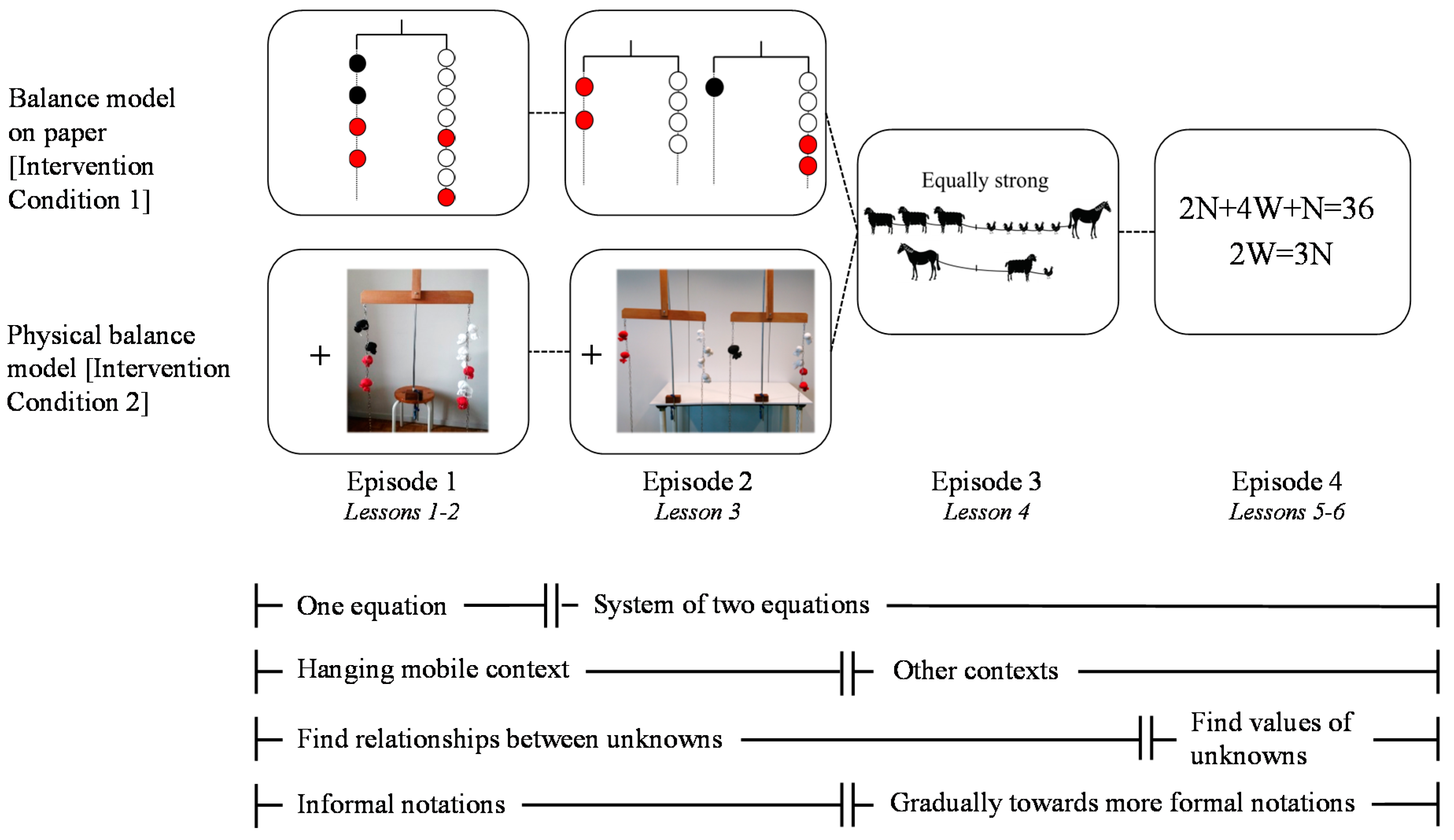
2.3. Intervention Program

The intervention program consisted of a six-lesson teaching sequence on solving linear equations (see also, [15]). In the beginning of this teaching sequence, the focus was on solving informal linear equations, that is, equations posed in informal contexts that students directly have a good understanding of. Over the course of the teaching sequence, more formal equations were introduced gradually. The teaching sequence could be clustered into four episodes based on the focus and content of the lessons (see Figure 1). In the first episode, students could develop informal algebraic strategies related to linear equation solving. Instead of the teacher transferring the strategies to the students, the students were active participants in developing the strategies. Students worked in small groups (2–3 students) using a hanging mobile as balance model and reasoned about relationships between unknowns. Their main task was to discover all possible ways to maintain the balance of the mobile (i.e., the equality). Students could, for example, exchange the balls of the left and right side of the mobile to figure out that both sides are interchangeable (i.e., apply a restructuring strategy), take away similar balls from both sides (i.e., apply an isolation strategy), or substitute one color of balls with another color and as such make use of the relationship between different unknowns (i.e., apply a substitution strategy). During the ensuing classroom discussion, students could mention all possibilities they discovered to maintain the balance of the mobile. The teacher wrote students’ ideas on the blackboard, which resulted in an overview of the various possibilities. Students’ own wordings were used in this overview (e.g., “change one color of bags by bags of another color” instead of “substitution”). From Episode 2 on, the information from two hanging mobiles had to be combined to discover new relationships between unknowns. At this time, students had to reason about a system of informal equations in the context of the hanging mobile. In Episode 3, problems were posed in new informal contexts which are often used for eliciting algebraic reasoning, such as a tug-of-war situation (see e.g., [45]). After a classroom discussion about equality being crucial in both the familiar context (the hanging mobile) and the new context (the tug-of-war situation), all possible strategies for maintaining this equality were discussed. Then, students were again invited to discover relationships between unknowns in this new context. In the example of the tug-of-war situation presented in Figure 1, students could, for example, apply a substitution strategy and replace one horse in the first informal equation by a sheep and a chicken (on the basis of the second equation), and take away a sheep from both sides in other to isolate the chickens on the right side of the equation. Moreover, in this third episode, students were gradually challenged to use more symbolic notations when writing down their reasoning. Finally, in Episode 4, students reasoned about systems of formal linear equations. The resemblance between the familiar contexts and the new context was discussed again, as well as the meaning of the algebraic symbols (e.g., what does W stand for?). Then, the students’ task was to use all previously discovered strategies for maintaining the equality of an equation, with the goal to combine the information of both symbolically notated equations in order to determine the values of the unknowns. In the example of the system of two formal linear equations presented in Figure 1, students could, for example, restructure the first equation by combining 2N and N into 3N, resulting in 3N + 4W = 36, then substitute 3N by 2W on the basis of the second equations (resulting in 6W = 36), and then further isolate the unknown W by dividing both sides by 6.

2.4. Measures

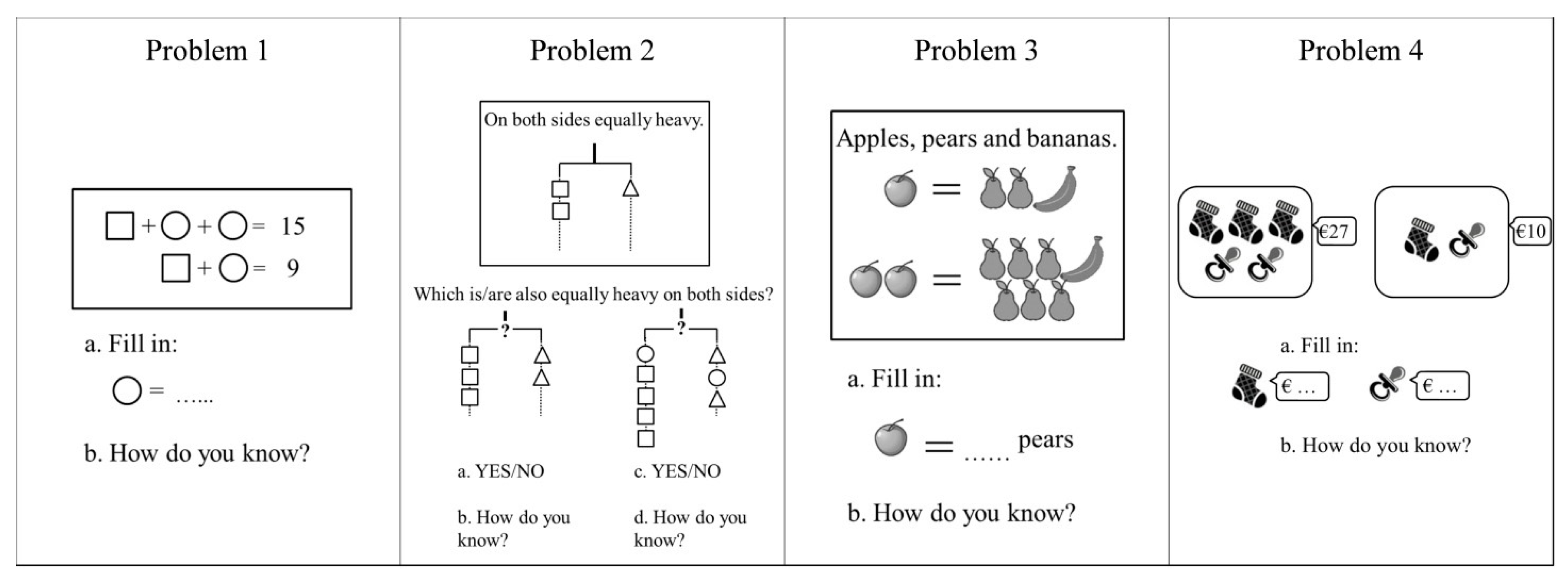
2.4.1. Algebraic Reasoning

Students’ algebraic reasoning related to solving linear equations was assessed by a paper-and-pencil test. Open-ended problems were used to explicitly invite students to explain their thinking and thus reveal their reasoning. The test consisted of four problems in which students had to solve (a system of) linear equations. The four problems were part of a larger test that also included problems in two other mathematical domains, namely graphing (four) and probability (five). In this study, we only focus on the problems on linear equation solving.
The problems on linear equation solving (see Figure 2) were formulated in such a way that prior instruction in formal linear equation solving was not necessary to solve the problems. Information presented in two informal equations had to be combined. In Problems 1, 3, and 4 a system of two linear equations was presented which had to be solved; in Problem 2 the information from a given equation had to be compared with the information from two other equations. Whereas in Problems 1 and 4 the goal was to find the value of the unknowns, in Problems 2 and 3 the task was to discover a relationship between unknowns. The algebraic strategies of restructuring, isolation, and substitution were needed to solve the problems.

Coding

Students’ reasoning on each of the problems was categorized by means of a coding scheme. An iterative process, inspired by the constant comparative method [46], was used for its development. The first version of the coding scheme was developed by taking the work of a couple of students. We first analyzed students’ reasoning based on the strategies of restructuring, isolation, and substitution when solving the systems of equations. When students used the strategies of restructuring or isolation, this usually meant that in their reasoning they only integrated the information from one of the two equations in the problem. When students made use of the more advanced substitution strategy, they generally combined the information from both given equations in their reasoning. Sometimes substitution was separately used, but more often in combination with the restructuring and isolation strategies. Another strategy which was often used when combining both equations was the strategy of elimination of unknowns by subtracting one equation from the other.
There appeared to be an intricate relation between the use of relevant algebraic strategies in students’ reasoning and the number of equations they referred to while describing their solution of the problem. Focusing on the number of equations in students’ reasoning turned out to be the most reliable way of coding students’ written work, as this was almost always quite clearly visible, whereas the algebraic strategies were much more indirectly mentioned. In the end, we therefore decided to distinguish between students who did not use any of the two given equations in their reasoning (Level R0), students who reasoned on the basis of only one of the two given equations (Level R1), and students who reasoned on the basis of both given equations by combining the information of both of them (Level R2). Importantly, these levels of students’ algebraic reasoning thus reflected both the straightforward number of equations they referred to in their reasoning and also the depth of their reasoning by the use of the algebraic strategies.
After several rounds of coding, 100% consensus was reached between the researchers and a final coding scheme was established, which was used for a final round of data coding. The final coding scheme, with examples of student responses for each problem and each level of reasoning, can be found in Appendix A. Examples of responses in which students did not show the use of any of the equations in their reasoning (Level R0) were: “I made a guess”, “Because I think this should be the answer”, “?”, or “I have no clue”. Student responses in which only one of both given equations was used (Level R1), for example in Problem 4 (see Figure 2), only referred to one equation, such as “5 + 5 = 10, so both must be €5”, “this fits in the second one, because 7 + 3 = 10”, or “in the first one you see 3 socks and 2 pacifiers must be 27, so one sock = 5 and the pacifier = 6”. Examples of responses in which students reasoned on the basis of both given equations (Level R2) were in Problem 4, explanations like “3 × 7 = 21, 2 × 3 = 6, 6 + 21 = 27. And 7 + 3 = 10. So, this must be the answer”, or “€10 + €10 = €20. Then one sock is left, so the sock must be €7. Then the pacifier =€3”. When a student did not provide any reasoning, this was coded as missing.
Inter-rater reliability was established by having an independent second rater recode the responses of 10% of the students. Two or three students were randomly drawn from each class, resulting in a sample of 21 students (84 responses for each problem, 336 responses in total). Inter-rater reliability between coders was high (Cohen’s kappa = .92).

2.4.2. General Reasoning Ability

An abbreviated version of Raven’s Standard Progressive Matrices (SPM) [47], consisting of 18 items [48], was used as a measure of general reasoning ability. The items, which increased in difficulty, consisted of diagrams with one part missing. Students have to reason which part is missing, before selecting this missing part to complete the design among six or eight alternatives. Answers were scored as incorrect (0) or correct (1), resulting in the minimum score of 0 and the maximum score of 18.

2.4.3. General Mathematics Performance

Students’ general mathematics performance was measured by the CITO Monitoring System, a Dutch standardized test for different subjects and grade levels [49]. The end-term scores of Grade 4 were obtained.

2.5. Research Design and Procedures

The study was approved by the ethical committee of the University. A staged comparison design with two intervention conditions and one control condition was used (see Table 1). Making use of this staged design made it possible that the same teacher taught all experimental lessons in both intervention conditions. We distinguished three cohorts which differed in the timing of the teaching sequence, and a fourth cohort with the control condition who did not receive algebra instruction but lessons on probability. Each of the three cohorts in the intervention conditions was made up of matched pairs of classes, based on characteristics such as the location of the school, the type of school, and the percentages of students going to particular levels of secondary education. Subsequently, within each pair, the classes were randomly divided over the two intervention conditions.
Over the school year, the students’ algebraic reasoning related to solving linear equations was assessed four times by means of the same algebraic reasoning test, with approximately two months in between. In this way, the algebraic reasoning of students in each cohort was measured before and after participating in the teaching sequence. The teaching sequence consisted of six lessons, of about 50 min each. The students were taught one lesson a week, during six consecutive weeks. The lessons in both intervention conditions (Cohorts 1–3) were taught by the first author of this paper, while the probability lessons in the control condition (Cohort 4) were taught by another researcher from the same research group. Raven’s SPM was administered in each class before the beginning of the study.

2.6. Data Analysis

2.6.1. Qualitative Analysis

To get insight into students’ development in reasoning, we first identified for the whole sample, for each cohort of students, and for each problem the most prevalent patterns of reasoning. The work of two students, whose patterns of reasoning were most prevalent (and thus representative) on that problem, was further analyzed and discussed.
We then compared all students’ use of the model after participating in an intervention with either a balance model on paper or a physical balance model. In this way, we could frame the use of the balance model of the two students whose reasoning was analyzed more deeply, and we could shed more light on the effects of working with different representations of the balance model. On the measurement directly after the intervention we looked into (1) whether students explicitly used a representation of the balance model (i.e., a drawing of the model) in their reasoning, and (2) whether students implicitly used the model as shown in their use of the algebraic strategies. This was only done for Problems 1, 3, and 4, because in Problem 2 the representation of a balance model was already part of the question. Because not all algebraic strategies were equally easy to discern in the students’ reasoning we decided to focus only on the more advanced algebraic strategies for combining both equations: substitution of a part of one equation on the basis of the information from the other or subtracting one equation from the other in order to eliminate unknowns.

2.6.2. Quantitative Analysis

Descriptive Statistics

Analyses of variance (ANOVAs) were performed to compare the three conditions on general reasoning ability and general mathematics performance. Proportions of each level of reasoning (R0, R1, R2) on the algebraic reasoning test were calculated for each cohort of each condition on each of the measurements.

Multi-Group Latent Variable Growth Curve Modeling

Latent variable growth curve modeling (LGM) was used to model students’ development in algebraic reasoning about linear equations over the four measurements. LGM is a powerful and flexible technique for modeling longitudinal change using repeated measures [50]. The core of such an LGM is a latent ability, in this case students’ reasoning about linear equations, that is different for each participant (inter-individual differences), but which also possibly changes within participants (intra-individual differences) over the four measurements. A cohort sequential multi-group LGM [51] was used in this study, with the cohorts as groups.
Item response theory (IRT) was used to map the likelihood of a level of reasoning (Level R0, R1, or R2) onto students’ latent algebraic reasoning ability. This latent ability was modeled as the combination of four partial effects: (1) The intercept effect: The baseline over all measurements; (2) The slope effect: The linear change from one measurement to the next; (3) The intervention effect: The effect of the intervention could only influence the score in the measurements following the intervention (e.g., when the intervention took place between M1 and M2, this would influence M2, M3, and M4); (4) The weakening effect: The weakening of the effect of the intervention could only influence the score in the delayed measurements after the intervention (e.g., when the intervention took place between M1 and M2, this would influence M3 and M4). The possibility existed that there were baseline differences in ability between the different cohorts in our study. Therefore, differences between the intercepts of the different cohorts were allowed. Because of the different timing of the intervention, the loadings for intervention and weakening also systematically differed for Cohorts 1–3. Because there was no intervention in Cohort 4, we did not include an intervention or weakening effect in this cohort. All other parameters were modelled exactly the same in all cohorts. Using LGM thus allowed us to disentangle students’ possible (linear) development over the four measurements (represented by the intercept and the slope) from the intervention effect.
In addition to these partial effects, three predictors were added to the model: (a) Condition was added as a dummy predictor of the intervention effect (coded as −1 and 1, for Intervention Conditions 1 and 2, respectively); (b) A measure of general reasoning ability [47,48] was added in a centered form as a predictor of the intercept; (c) A measure of general mathematics performance [49] was added in a centered form as a predictor of the intercept.
The model was fitted in Mplus 8 [52], with the weighted least squares means and variances adjusted estimator (WLS-MV). Following commonly applied cut-off criteria, model fit was considered acceptable with the Root Mean Square Error of Approximation (RMSEA) below .08 and the Comparative Fit Index (CFI) and the Tucker–Lewis Index (TLI) above .90 [53]. A PROBIT link was used, which means that differences between difficulty and ability are expressed in units that refer to a standard normal distribution with a mean of zero, with units representing standard deviations.

2.6.3. Missing Data

There were four students for whom one of the measurements M1-M3 was completely missing, while subsequent measure(s) were present. We reasoned that the baseline linear change (i.e., the slope effect) could be estimated less reliably when one of the measurements in between was missing. We therefore decided for each case to replace the missing measurement by the subsequent measurement. More specifically, M2 of one student from Cohort 1 was missing; M3 was used as if it were M2 (as the measurement directly after the intervention) and M4 as M3. The same procedure was applied to the three other students, belonging to the control condition, of which M1, M3, and M3 were missing, respectively. Class averages were calculated and imputed for students’ missing general mathematics performance scores.

3. Results

In this results section, we first give an idea of what students’ development in algebraic reasoning included by providing a qualitative analysis of two students’ reasoning over the measurements and their use of the balance model. The patterns of reasoning of these two students were most prevalent (and thus representative) on these two problems. Next, we investigate whether the results of these two students can be generalized to the whole sample. We qualitatively investigate the effect of working with different representations of the balance model on all students’ use of this model when solving systems of informal linear equations in other contexts (i.e., contexts not related to the balance model). We distinguish between explicit use (i.e., using a representation of the model) and implicit use (i.e., using algebraic strategies).
After presenting the results of this qualitative analysis, we continue with the findings of the quantitative analysis of students’ level of reasoning. Here, we investigate the effects of using the balance model on students’ levels of reasoning in both the short term and the long term. In addition, we consider the effects of the students’ working with a physical versus a pictorial representation of the balance model on their levels of reasoning.

3.1. Results from the Qualitative Analysis of Students’ Reasoning

3.1.1. Case 1—Noah

Noah participated in Cohort 1 and worked with the hanging mobile on paper (Intervention Condition 1). His reasoning on this problem consisted of the pattern R1-R2-R2-R2, a pattern which was the most prevalent in this cohort and displayed by 9% of the students. Noah’s answers and his reasoning on the measurements right before the intervention (i.e., the pretest M1) and right after the intervention (i.e., the direct posttest M2) are displayed in Figure 3.
On the measurement before the intervention, Noah based his answer on the first equation, in which two pears are displayed as part of the equation. He ignored the rest of the first equation and the entire second equation. This reasoning was therefore categorized as Level R1 (reasoning on the basis of only one equation). No algebraic strategies came to the fore in his reasoning. On the measurement directly after the intervention, Noah first converted both equations into symbols. Subsequently, he showed that the first equation could be subtracted from the second equation, revealing the relationship between the apples and the pears. This reasoning was categorized as Level R2 (reasoning on the basis of both equations). Noah’s answer on this problem can be seen as a clear demonstration of the effect of the intervention. In his reasoning he showed understanding of how to combine the information of both equations in the problem: by subtracting one equation from the other, one unknown was isolated. Moreover, he displayed his algebraic reasoning by making use of letters.

3.1.2. Case 2—Lea

As a second example, we zoom in on the reasoning of Lea, a student from Cohort 3 who worked with the physical hanging mobile (Intervention Condition 2). Lea demonstrated a pattern of reasoning consisting of only Level R2 on all four measurements of Problem 4. This pattern was most prevalent for this problem in Cohorts 1 and 3 (displayed by 23% and 14% of the students respectively). Lea’s answers on M1–M3 were very similar; her reasoning on the measurement before the intervention (i.e., the pretest M3) and after the intervention (i.e., the direct posttest M4) is shown in Figure 4.
On the measurement prior to the intervention, Lea substituted the values in both equations and thus showed that these values add up to the right amounts of €10 and €27. Because she made use of both given equations, her reasoning was categorized as the highest level of reasoning (Level R2). On the measurement after partaking in the teaching sequence, Lea started with converting both equations into hanging mobiles, making her reasoning visible. She then doubled the second equation and subtracted the value of 20 from the first equation. In this way, she isolated the sock and determined its value (€7). Subsequently, she substituted this value of 7 for one sock in the first equation to reveal that two pacifiers must be equal to €6 so one pacifier must be €3. This reasoning was again categorized as Level R2. Although the effect of the intervention is not directly visible in Lea’s pattern of reasoning levels, we do see an effect when we zoom in on the extensiveness and completeness of her reasoning: whereas Lea in M1–M3 proved the correctness of her answer by substituting both values in both equations, in M4 she clearly made use of various algebraic strategies to come to her answer. She isolated one unknown by subtracting the second equation two times from the first equation and used the strategy of substituting unknowns by values. By converting the equations into hanging mobiles, which she used in combination with pre-formal algebraic symbols, she moreover showed her ability to incorporate different representations into her reasoning and her flexibility in switching between these representations.
For both students, the effect of working with the balance model during the intervention was visible in their algebraic reasoning on the measurement directly following the intervention. Both students, either after working with the model on paper (Noah) or with the physical model (Lea), displayed algebraic reasoning by eliminating unknowns through subtracting one equation from the other (i.e., they took away things on both sides of one equation on the basis of the other equation). Moreover, Lea explicitly made use of the model of the balance in her reasoning.
Examination of the work of all students who worked with the balance model on paper (Intervention Condition 1) revealed that 27 students (40%) made use in at least one of the problems of an advanced algebraic strategy (i.e., substitution or elimination) for combining both equations (like Noah). Only one student (1%) in this intervention condition explicitly made use of the representation of the balance model in their reasoning. On the contrary, 39 students (60%) who worked with the physical balance model (Intervention Condition 2) used at least once such an advanced algebraic strategy for combining both equations, and, moreover, 11 students (17%) explicitly used the model of the balance in their reasoning (like Lea).
So far, this analysis demonstrates differences between intervention conditions as regards the use of the balance model on the measurement after the intervention. There might also be differences between both conditions when focusing on students’ levels of reasoning. An analysis of these differences is reported in the next section.

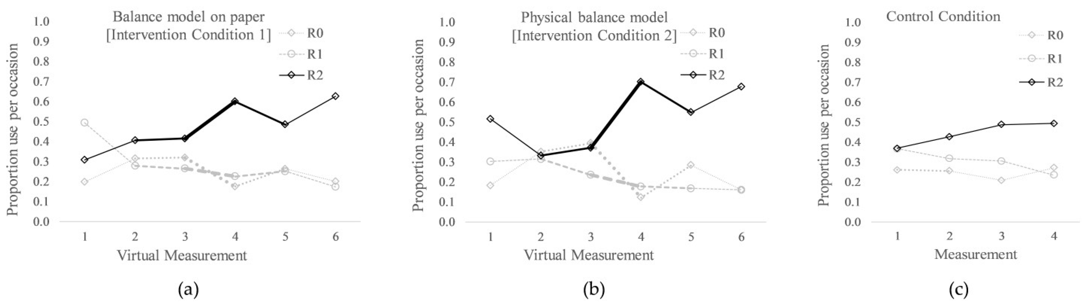
3.2. Results from the Quantitative Analysis of Students’ Reasoning

In this section, we will further analyze students’ development in algebraic reasoning. We will start with providing the descriptive statistics, and then present our LGM model

3.2.1. Descriptive Statistics

Students’ general reasoning ability (F(2, 209) = 1.11, p = .331, partial ƞ2 = .011) and general mathematics performance (F(2, 209) = 1.92, p = .149, partial ƞ2 = .018) did not significantly differ between students in the three conditions (see Table 2).
The proportion of each level of reasoning on the four algebraic reasoning problems is for each condition shown in Figure 5. To allow for direct (visual) comparison of the change in reasoning for all cohorts of the intervention conditions, virtual measurements were created. That is, students in Cohort 1 were depicted as having participated in virtual measurements 3–6, students in Cohort 2 as having participated in virtual measurements 2–5, and students in Cohort 3 as having participated in virtual measurements 1–4. In this way, virtual measurement 3 is identified with the measurement directly before the intervention for all cohorts (i.e., the pretest) and virtual measurement 4 with the measurement directly after the intervention (i.e., the direct posttest; see Figure 5a,b). In both intervention conditions, the proportion of levels of reasoning R0 and R1 decreased after the intervention compared to before the intervention, while the proportion of level of reasoning R2 increased. Thus, in both intervention conditions students showed more reasoning on the basis of both linear equations after participating in the teaching sequence. Moreover, the proportion of Level R2 increased more in Intervention Condition 2 (.33 increase in proportion) than in the cohorts of Intervention Condition 1 (.18 increase in proportion). Figure 5c shows the proportion of each level of reasoning on the four measurements for the Control Condition. The proportions of levels of reasoning in the Control Condition remained more or less stable.

3.2.2. Multi-Group Latent Growth Model

A multi-group LGM with a PROBIT link was fitted to investigate the overall effect of the intervention on students’ reasoning ability in both the short term and the long term and to investigate the effect of the two different representations of the balance model on this reasoning ability. The model with an intercept, slope, intervention effect, and weakening effect, condition as predictor of the intervention effect and general reasoning ability as predictor of the intercept had an acceptable fit (RMSEA = .066, 90% CI [.050–.080], CFI = .926, TLI = .937). Adding general mathematics performance as a predictor resulted in a deterioration of the fit and was therefore disregarded in this analysis. Table 3 shows the parameter estimates of this model. The overall effect of the intervention on students’ reasoning ability was significant (M = 0.67, p < .001). Students’ algebraic reasoning thus improved after partaking in the teaching sequence. This effect showed weakening on the delayed measures after the intervention (M = −0.31, p = .001), which means that students’ level of algebraic reasoning decreased a little in the long term. The differential effect of condition (physical vs. pictorial balance model) on the intervention effect turned out to be nonsignificant (β = .33, p = .136). In other words, the representation of the balance model did not differentially affect students’ reasoning. Lastly, general reasoning ability was a significant predictor of students’ baseline reasoning ability (i.e., the intercept, β = .34, p < .001), which means that a higher general reasoning ability was associated with a higher baseline level of algebraic reasoning.
In order to gauge the effect size of the intervention, it is helpful to visualize the results. As an illustration, Figure 6a shows a standard normal distribution (as required for a PROBIT model) representing the hypothetical algebraic reasoning ability of all students on Problem 1 at the measurement directly before the intervention. The total area under the curve is one and is divided in three parts, separated by so-called thresholds, which reflect the likelihood of reasoning in accordance with Levels R0, R1, and R2, respectively. At the measurement just after the intervention, the algebraic reasoning abilities have changed and the curve in the figure has shifted to the right (see Figure 6b). The thresholds do not change. Due to the intervention, the likelihood of reasoning in accordance with Level R0 decreases, as can be seen in Figure 6, while the likelihood of reasoning in accordance with Level R2 increases after the intervention. In other words, this figure visualizes that after partaking in the teaching sequence students’ reasoning improves: fewer students use none of the given equations in their reasoning (Level R0), somewhat fewer students reason on the basis of only one of the given equations (Level R1), and more students combine the information of both equations in their reasoning (Level R2).
The effect size of the intervention determined by the whole test can be computed straightforwardly from the model parameters in Table 3. As explained earlier, a score is based on four components: the intercept, the slope, the intervention effect, and the weakening effect. As the intercept only influences the first measurement and the weakening effect is still zero at the measurement directly after the intervention, the effect size of the score gain (Cohen’s d) is reflected by the sum of the intervention and the slope effect from Table 3: .67 + .06 = .73.

4. Discussion

In this study, we investigated the effects of two learning environments consisting of a teaching sequence with a balance model on the development of primary school students’ algebraic reasoning related to linear equation solving. The balance models in these learning environments were implemented in two different representations (dynamic physical vs. static pictorial on paper). The development of students’ algebraic reasoning was examined through four assessments over the school year, with students participating in the teaching sequence between two of these measurements. In the assessments, students answered four open-ended tasks, each representing a system of informal linear equations. The sample in this study had no prior instruction on linear equations.
Our results show that fifth-grade students who participated in an intervention based on the balance model showed higher levels of algebraic reasoning when solving systems of informal linear equations. Students improved in their ability to reason by combining the information of both equations (Level R2), instead of reasoning on the basis of only one of the two given equations (Level R1) or none of the given equations (Level R0). This highest level of reasoning was displayed more frequently after the intervention (65%) than before (39%). These results underscore previous research showing that primary school students’ algebraic reasoning about (systems of) linear equations can be fostered [6,7,54,55]. It moreover underlines the suitability of the balance model for stimulating and structuring this reasoning (see also, e.g., [15,27,28,29,37]). In addition, we also systematically investigated the development in reasoning of all students by making use of repeated measurements. This allowed us to examine both the short-term effects of the intervention and its long-term effects: resulting in the finding of a small fading out of the intervention effect.
However, our main interest was whether a static pictorial representation of a balance model had a different effect on the development of students’ algebraic reasoning than a physical balance model which students can manipulate and which tilts in response to students’ actions. We expected students’ perceptual-motor experiences with the physical balance model to be beneficial for their understanding of the abstract mathematical concept of equality in an equation, in line with, e.g., [25,40,42], which we supposed to positively influence their reasoning about linear equations. Qualitative analyses of students’ written responses on the measurement directly after the intervention showed that students who worked with the physical balance model more frequently used the balance model when solving systems of informal linear equations in contexts not related to the balance model than students who worked with the model on paper. This use of the model was either explicit, by making use of the representation of the model, or implicit, by making use of substitution of a part of one equation on the basis of the information from the other, or subtracting one equation from the other in order to eliminate unknowns. For students who worked with the physical balance model, 17% used the representation of the model in their reasoning and 60% used advanced algebraic strategies, compared to only 1% and 40% of the students who worked with the model on paper. However, although the descriptive values also suggested a larger improvement in level of reasoning for students who worked with the physical balance model compared to students who worked with the model on paper, the LGM analysis did not yield significant differences in the development of students’ levels of algebraic reasoning about equations.
There are several possible explanations for this nonsignificant finding. The teaching sequence in both intervention conditions might have been too similar to affect students’ level of algebraic reasoning differently. After all, apart from the used representation, students in both conditions were taught by means of the same didactical model. Such models are meant to elicit students’ growth in understanding of mathematics [56]. Through the balance model, students in both types of intervention were primed to the equality concept, which is crucial to come up with strategies to solve linear equations and which can assist students to bring the focus on an equation as representing a mathematical structure that links two different algebraic expressions. Possibly, the balance model is a very strong didactical model, which, independent of the representation of the model, is very accessible for students and can help them make sense of the problem situation. Additionally, the difference between both teaching sequences was present mainly in the first three lessons, with students working with only a balance model on paper or in addition to a physical balance model. This period of three lessons might have been too short to induce a different effect on students’ reasoning. Lastly, it is also possible that both representations evoke the idea of balance in line with [39,40,41], which is strongly grounded in previous physical experiences [42,43]. Direct perceptual-motor experiences with the physical balance model, or indirect experiences through mental simulation or predicting whether the model on paper will be in or out of balance, can result in the same neural activation patterns (see also, e.g., [57]).
These explanations for the absence of a significant difference between the intervention conditions as regards students’ levels of reasoning are in contrast with the differences between conditions as regards students’ use of the balance model, reflected by either their use of a representation of the model and/or their use of advanced algebraic strategies. A possible explanation for this discrepancy is that different representations of the balance model do affect students’ algebraic reasoning differently, but only on such a detailed level that our coding scheme was not able to capture these differences. Although our three-level coding scheme proved to be suitable to capture students’ level of algebraic reasoning (with a high inter-rater reliability) and although the different levels of reasoning did reflect, to a certain extent, the depth of students’ reasoning by the use of algebraic strategies, we, in the end, did lose some of the richness in students’ reasoning by means of this straightforward way of coding. Lea’s pattern of reasoning provides a good example: although she consistently showed reasoning on the basis of both equations (Level R2), her reasoning after participating in the teaching sequence was much more elaborate and she clearly used more algebraic strategies (or at least she was better able to demonstrate her use of algebraic strategies in her written response). Also, because we did not include think-aloud protocols or other types of live registration of reasoning, we might not have captured the students’ full reasoning. We recommend further research to investigate the effects of different representations of the balance model on students’ reasoning while making use of live registration of students’ reasoning.
Alternatively, because of practical reasons (all lessons were taught by the same teacher) we made use of different cohorts in our study. Within each cohort of each intervention condition we included only one class. This might have resulted in too little power to detect differences in levels of reasoning between conditions using the LGM analysis. The fact that all cohorts of students working with the physical balance model showed higher learning gains could be an indication of this. Ideally, we would have included more than 212 students in our study. This probably would have resulted in a better fitting model and more power to detect potential effects. A design without cohorts or with multiple classes within each cohort would then be preferable to enhance the power of the study.
When interpreting the results of our study, one should also keep in mind its quasi-experimental nature. There was no random assignment of students to conditions. However, we did control for initial differences between classes in our analyses, by including general reasoning ability and general mathematics ability as covariates. Moreover, quasi-experimental designs are considered very appropriate for testing the effectiveness of interventions in natural educational environments [58]. On the other hand, the study design also has several strengths. First, our staged comparison design with multiple cohorts allowed us to investigate not only the short-term but also the long-term effects of the intervention on students’ reasoning. It also created the possibility to take into account the effect of repeatedly assessing students’ algebraic reasoning. Second, mixed methods (i.e., quantitative and qualitative analyses) could be used. We went beyond only looking at the correctness of all students’ answers, which is often done from a pragmatic point of view, and instead focused on students’ reasoning. LGM was subsequently used to model the development of students’ algebraic reasoning ability. Lastly, this study could take place in an authentic classroom setting. The high ecological validity makes the results of our study quite easy to translate to educational practice.
In the current study, we demonstrated the effectiveness of a learning environment with the balance model, in a whole-classroom setting, on primary school students’ reasoning about solving systems of informal linear equations. Using this model to elicit algebraic reasoning aligns with the objective to commence with stimulating such reasoning in primary school classrooms [2]. No significant differences were found between using a balance model on paper or a physical balance model on the development of students’ level of reasoning, suggesting that the representation of the model does not play a role. However, having a closer look at students’ reasoning revealed that students who worked with the physical balance model more often made use of the balance model, either by making use of the representation of the model or by making use of algebraic strategies such as substitution or elimination, when solving systems of informal linear equations. This suggests that different representations of the balance model might play a different role in individual learning processes. We recommend for future research to address this discrepancy in findings and to further investigate the possibility that different representations of the balance model might affect students’ algebraic reasoning differently, for example by making use of live registration of students’ reasoning.

Author Contributions

Conceptualization, formal analysis, methodology, writing—original draft preparation, writing—review and editing: M.O., M.v.d.H-P., M.V., J.B. and A.H.; project administration, resources: M.O., M.v.d.H-P. and M.V.; funding acquisition: M.v.d.H-P. and J.B.; software: J.B.; investigation: M.O.; supervision: M.v.d.H-P., M.V. and A.H. All authors have read and agreed to the published version of the manuscript.

Funding

This research was funded by The Netherlands Initiative for Education Research, Grant NRO: Project 405-14-303.

Conflicts of Interest

The authors declare no conflict of interest.

Appendix A

Table A1. Coding scheme with examples of student responses for each problem and each level; text in between square brackets is added as a clarification.
Level of ReasoningDescriptionSubtypesProblem 1
Education 10 00163 i001
Problem 2
Education 10 00163 i002
Problem 3
Education 10 00163 i003
Problem 4
Education 10 00163 i004
R0Student does not use one any of the given equationsR0_empty[no response]IdemIdemIdem
R0_don’t know
-
“I don’t understand it”
-
“I don’t know”
-
“?”
IdemIdemIdem
R0_just know
-
“That’s what I think”
-
“I just see it right away”
IdemIdemIdem
R0_repeat given equation(s) or question(s)-
-
“3 squares = 2 triangles” [question a]
-
“they use the same figures as in the example”
-
“that’s what is written above”
-
“because the example shows apple = pear + pear + banana”
-
“look at the picture”
-
R0_repeat answer(s)--
-
“one apple = 2 pears”
-
“sock = 7, pacifier = 3”
-
“because the sock costs 5 euros and the pacifier costs 2 euros”
R0_general description
-
“just look at the problem for a while”
-
“I made a guess”
-
“I just tried something”
IdemIdemIdem
R1Student reasons on the basis of only one of the two given equations R1_without showing strategy
-
“3 + 6 = 9”
-
“5 + 5 + 5 = 15”
-
“2 squares are 1 triangle, and that’s impossible here”
-
“one square is missing” [question a]
-
”pear = 1, banana = 2, apple = 4, 4 = 1 + 1 + 2”
-
“one banana = 2 pears, so one apple equals 2 + 2 = 4 pears”
-
“5 + 5 = 10”
-
“3 socks = 21, 2 pacifiers = 6”
-
“2 × 9 = 18, 3 × 3 = 9, 18 + 9 = 27”
R1_with showing strategy
-
“take half of 9”
-
“divide 15 by 3”
-
“it is the same as the example, only on both side there is one extra figure so it’s still equal”
-
“you can see it in the upper one that one apple is two pears”
-
“2 apples are six pears so if you take half you know one apple is three pears”
-
“take half of 10”
-
“try different combinations to make 10”
R2Student reasons on the basis of both given equations by combining the information of both of themR2_without showing strategy
-
“3 + 6 = 9, 3 + 6 + 6 = 15”
-
“when you add 3 and 6 it is 9, and 3 plus 6 plus 6 is fifteen”
-
“if you fill in 3 and 6 in both, it fits”
-
“you need one additional square [question a]; 4 squares = 2 triangles and circle = circle”
-
“1 triangle = 2 squares and the circles are the same”
-
”pear = 1, banana = 2, apple = 4, 4 = 1 + 1 + 2, 8 = 1 + 1 + 1 + 1 + 1 + 1 + 2”
-
“if a banana = 2 pears, then one apple = 4 pears and 2 apples = 8 pears”
-
“7 + 3 = 10, 7 + 7 + 7 + 3 +3 = 27”
-
“3 socks = 21, 2 pacifiers = 6, 7 + 3 = 10”
-
“I tried these values in both examples and this was OK”
R2_with showing strategy
-
“square + circle = 9, than you need 6 more to have 15. So circle must be 6”
-
“15 − 9 = 6”
-
“square + circle = 9, so 9 + circle = 15”
-
“I started with 4 and 5, that did not fit in both calculations, so then I tried 3 and 6. That worked well”
-
“1 triangle = 2 squares, so 2 triangles = 4 squares, 1 circle = 1 circle”
-
“the circles are equal so you can remove them. Then there are 2 triangles and 4 squares left, divided by 2 equals 1 triangle and 2 squares. So that’s correct”
-
“the two circles are equally heavy and if you double the example you get 4 squares = 2 triangles”
-
“if you subtract 2 pears and 1 banana from the second one, four pears remain. So one apple is four pears”
-
“if you double the apples the other part must also be doubled. So that must be four pears and two bananas. But there are six pears and one banana. So one banana = two pears. So an apple = 2 + 2 = 4 pears”
-
“two pears and 1 banana can be replaced by one apple, so then the other apple equals 4 pears”
-
“27 − 10 − 10 = 7, so pacifier = 7, sock must be 3.”
-
“take away 10 two times, then 7 remains. 3 × 7 = 21, so sock = 3”
-
“One sock and one pacifier = 10, so 10 + 10 = 20, so pacifier = 7”
-
“I first tried 9 & 1, then 8 & 2, then 7 & 3. 7 & 3 worked for both questions”

References

  1. Cai, J.; Jakabcsin, M.S.; Lane, S. Assessing students’ mathematical communication. Sch. Sci. Math. 1996, 96, 238–246. [Google Scholar] [CrossRef]
  2. National Council of Teachers of Mathematics [NCTM]. Principles and Standards for School Mathematics; NCTM: Reston, VA, USA, 2000. [Google Scholar]
  3. Stein, M.K.; Grover, B.W.; Henningsen, M. Building student capacity for mathematical thinking and reasoning: An analysis of mathematical tasks used in reform classrooms. Am. Educ. Res. J. 1996, 33, 455–488. [Google Scholar] [CrossRef]
  4. Thom, J.S. Nurturing mathematical reasoning. Teach. Child. Math. 2011, 18, 234–243. [Google Scholar] [CrossRef]
  5. Kilpatrick, J.; Swafford, J.; Findell, B. Adding it up: Helping Children Learn Mathematics; National Research Council: Washington, DC, USA, 2001. [Google Scholar]
  6. Blanton, M.; Stephens, A.; Knuth, E.; Gardiner, A.M.; Isler, I.; Kim, J.S. The development of children’s algebraic thinking: The impact of a comprehensive early algebra intervention in third grade. J. Res. Math. Educ. 2015, 46, 39–87. [Google Scholar] [CrossRef]
  7. Brizuela, B.; Schliemann, A. Ten-year-old students solving linear equations. Learn. Math. 2004, 24, 33–40. [Google Scholar]
  8. Kaput, J.J.; Carraher, D.W.; Blanton, M.L. Algebra in the Early Grades; Lawrence Erlbaum Associates: New York, NY, USA, 2008. [Google Scholar]
  9. Blanton, M.L.; Kaput, J.J. Characterizing a classroom practice that promotes algebraic reasoning. J. Res. Math. Educ. 2005, 36, 412–446. [Google Scholar] [CrossRef]
  10. Cai, J.; Knuth, E. A global dialogue about early algebraization from multiple perspectives. In Early algebraization; Cai, J., Knuth, E., Eds.; Springer: New York, NY, USA, 2011. [Google Scholar]
  11. Blanton, M.; Schifter, D.; Inge, V.; Lofgren, P.; Willis, C.; Davis, F.; Confrey, J. Early algebra. In Algebra: Gateway to a Technological Future; Katz, J., Ed.; The Mathematical Association of America: Washington, DC, USA, 2007; pp. 7–15. [Google Scholar]
  12. Smith, J.P.; Thompson, P.W. Quantitative reasoning and the development of algebraic reasoning. In Algebra in the Early Grades; Kaput, J.J., Carraher, D.W., Blanton, M.L., Eds.; Lawrence Erlbaum Associates: New York, NY, USA, 2008; pp. 95–132. [Google Scholar]
  13. Stephens, A.C.; Fonger, N.; Strachota, S.; Isler, I.; Blanton, M.; Knuth, E.; Gardiner, A. A learning progression for elementary students’ functional thinking. Math. Think. Learn. 2017, 19, 143–166. [Google Scholar] [CrossRef]
  14. Goldenberg, P.E.; Mark, J.; Kang, J.; Fries, M.; Carter, C.J.; Cordner, T. Making Sense of Algebra: Developing Students’ Mathematical Habits of Mind; Heinemann: Portsmouth, NH, USA, 2015. [Google Scholar]
  15. Otten, M.; Van den Heuvel-Panhuizen, M.; Veldhuis, M.; Heinze, A. Developing algebraic reasoning in primary school using a hanging mobile as a learning supportive tool. J. Study Educ. Dev. 2019, 42, 615–663. [Google Scholar] [CrossRef]
  16. Jones, I.; Inglis, M.; Gilmore, C.; Dowens, M. Substitution and sameness: Two components of a relational conception of the equals sign. J. Exp. Child. Psychol. 2012, 113, 166–176. [Google Scholar] [CrossRef] [Green Version]
  17. Kieran, C. Concepts associated with the equality symbol. Educ. Stud. Math. 1981, 12, 317–326. [Google Scholar] [CrossRef]
  18. Bush, S.B.; Karp, K.S. Prerequisite algebra skills and associated misconceptions of middle grade students: A review. J. Math. Behav. 2013, 32, 613–632. [Google Scholar] [CrossRef]
  19. Kieran, C.; Pang, J.; Schifter, D.; Ng, S.F. Early Algebra: Research into its Nature, its Learning, its Teaching; Open access eBook; Springer: Berlin/Heidelberg, Germany, 2016. [Google Scholar] [CrossRef]
  20. Behr, M.; Erlwanger, S.; Nichols, E. How children view the equals sign. Math. Teach. 1980, 92, 13–15. [Google Scholar]
  21. Carpenter, T.P.; Franke, M.L.; Levi, L. Thinking Mathematically: Integrating Arithmetic and Algebra in Elementary School; Heinemann: Portsmouth, NH, USA, 2003. [Google Scholar]
  22. Falkner, K.P.; Levi, L.; Carpenter, T.P. Children’s understanding of equality: A foundation for algebra. Teach. Child. Math. 1999, 6, 232–236. [Google Scholar]
  23. Knuth, E.J.; Stephens, A.C.; McNeil, N.M.; Alibali, M.W. Does understanding the equal sign matter? Evidence from solving equations. J. Res. Math. Educ. 2006, 37, 297–312. [Google Scholar] [CrossRef]
  24. McNeil, N.M.; Alibali, M.W. Why won’t you change your mind? Knowledge of operational patterns hinders learning and performance on equations. Child Dev. 2005, 76, 883–899. [Google Scholar] [CrossRef]
  25. Antle, A.N.; Corness, G.; Bevans, A. Balancing justice: Comparing whole body and controller-based interaction for an abstract domain. Int. J. Arts Technol. 2013, 6, 388–409. [Google Scholar] [CrossRef]
  26. Figueira-Sampaio, A.S.; Santos, E.E.F.; Carrijo, G.A. A constructivist computational tool to assist in learning primary school mathematical equations. Comput. Educ. 2009, 53, 484–492. [Google Scholar] [CrossRef]
  27. Papadopoulos, I. Using mobile puzzles to exhibit certain algebraic habits of mind and demonstrate symbol-sense in primary school students. J. Math. Behav. 2019, 53, 210–227. [Google Scholar] [CrossRef]
  28. Suh, J.; Moyer, P.S. Developing students’ representational fluency using virtual and physical algebra balances. J. Comput. Math. Sci. Teach. 2007, 26, 155–173. [Google Scholar]
  29. Warren, E.; Cooper, T.J. Young children’s ability to use the balance strategy to solve for unknowns. Math. Educ. Res. J. 2005, 17, 58–72. [Google Scholar] [CrossRef]
  30. Alibali, M.W. How children change their minds: Strategy change can be gradual or abrupt. Dev. Psychol. 1999, 35, 127–145. [Google Scholar] [CrossRef] [PubMed]
  31. Kaplan, R.G.; Alon, S. Using technology to teach equivalence. Teach. Child. Math. 2013, 19, 382–389. [Google Scholar] [CrossRef]
  32. Bajwa, N.P.; Perry, M. Features of a pan balance that may support students’ developing understanding of mathematical equivalence. Math. Think. Learn. 2019. advance online publication. [Google Scholar] [CrossRef]
  33. Mann, R.L. Balancing act: The truth behind the equals sign. Teach. Child. Math. 2004, 11, 65–70. [Google Scholar]
  34. Anthony, G.; Burgess, T. Solving linear equations. In Algebra Teaching around the World; Leung, F., Park, K., Holton, D., Clarke, D., Eds.; Sense Publishers: Rotterdam, The Netherlands, 2014; pp. 17–37. [Google Scholar]
  35. Vlassis, J. The balance model: Hindrance or support for the solving of linear equations with one unknown. Educ. Stud. Math. 2002, 49, 341–359. [Google Scholar] [CrossRef]
  36. Cheeseman, J.; McDonough, A.; Golemac, D. Investigating children’s thinking about suspended balances. N. Z. J. Educ. Stud. 2017, 52, 143–158. [Google Scholar] [CrossRef]
  37. Otten, M.; Van den Heuvel-Panhuizen, M.; Veldhuis, M. The balance model for teaching linear equations: A systematic literature review. Int. J. STEM Educ. 2019, 6, 30–51. [Google Scholar] [CrossRef]
  38. Fyfe, E.R.; McNeil, N.M.; Borjas, S. Benefits of “concreteness fading” for children’s mathematics understanding. Learn. Instr. 2015, 35, 104–120. [Google Scholar] [CrossRef]
  39. Alibali, M.W.; Nathan, M.J. Embodiment in mathematics teaching and learning: Evidence from learners’ and teachers’ gestures. J. Learn. Sci. 2012, 21, 247–286. [Google Scholar] [CrossRef]
  40. Núñez, R.E.; Edwards, L.D.; Matos, J.F. Embodied cognition as grounding for situatedness and context in mathematics education. Educ. Stud. Math. 1999, 39, 45–65. [Google Scholar] [CrossRef]
  41. Wilson, M. Six views of embodied cognition. Psychon. Bull. Rev. 2002, 9, 625–636. [Google Scholar] [CrossRef] [PubMed]
  42. Alessandroni, N. Varieties of embodiment in cognitive science. Theory Psychol. 2018, 28, 1–22. [Google Scholar] [CrossRef]
  43. Gibbs, R.W., Jr. Embodiment and Cognitive Science; Cambridge University Press: Cambridge, UK, 2006. [Google Scholar]
  44. Carbonneau, K.J.; Marley, S.C.; Selig, J.P. A meta-analysis of the efficacy of teaching mathematics with concrete manipulatives. J. Educ. Psychol. 2013, 105, 380–400. [Google Scholar] [CrossRef]
  45. Kindt, M.; Abels, M.; Meyer, M.R.; Pligge, M.A. Comparing Quantities. In Mathematics in Context: A Connected Curriculum for Grades 5–8; National Center for Research in Mathematical Sciences Education, Freudenthal Institute, Ed.; Encyclopedia Brittanica Educational Corporation: Chicago, IL, USA, 1998. [Google Scholar]
  46. Glaser, B.G. The constant comparative method of qualitative analysis. Soc. Probl. 1965, 12, 436–445. [Google Scholar] [CrossRef]
  47. Raven, J.C.; Court, J.H.; Raven, J. Manual for Raven’s Standard Progressive Matrices and Vocabulary Scales; Oxford Psychologists Press: Oxford, UK, 1996. [Google Scholar]
  48. Bilker, W.B.; Hansen, J.A.; Brensinger, C.M.; Richard, J.; Gur, R.E.; Gur, R.C. Development of abbreviated nine-item forms of the Raven’s standard progressive matrices test. Assessment 2012, 19, 354–369. [Google Scholar] [CrossRef] [Green Version]
  49. Janssen, J.; Scheltens, F.; Kraemer, J.M. Leerling- en Onderwijsvolgsysteem Rekenen-wiskunde [Student Monitoring System Mathematics]; Cito: Arnhem, The Netherlands, 2005. [Google Scholar]
  50. Bollen, K.A.; Curran, P.J. Latent Curve Models; Wiley: Hoboken, NJ, USA, 2006. [Google Scholar]
  51. Duncan, T.E.; Duncan, S.C.; Strycker, L.A. An Introduction to Latent Variable Growth Curve Modeling, 2nd ed.; Lawrence Erlbaum Associates: Mahwah, NJ, USA, 2006. [Google Scholar]
  52. Muthén, L.K.; Muthén, B.O. Mplus User’s Guide, 8th ed.; Muthén & Muthén: Los Angeles, CA, USA, 1998–2017. [Google Scholar]
  53. Little, T.D. Longitudinal Structural Equation Modeling; Guildford Press: New York, NY, USA, 2013. [Google Scholar]
  54. Van Amerom, B.A. Focusing on informal strategies when linking arithmetic to early algebra. Educ. Stud. Math. 2003, 54, 63–75. [Google Scholar] [CrossRef]
  55. Van Reeuwijk, M. The role of Realistic Situations in Developing Tools for Solving Systems of Equations; Annual Meeting of the American Educational Research Association: San Francisco, CA, USA, 1995. [Google Scholar]
  56. Van den Heuvel-Panhuizen, M. The didactical use of models in realistic mathematics education: An example from a longitudinal trajectory on percentage. Educ. Stud. Math. 2003, 54, 9–35. [Google Scholar] [CrossRef]
  57. McCaffrey, T.; Matthews, P.G. An emoji is worth a thousand variables. Math. Teach. 2017, 111, 96–102. [Google Scholar] [CrossRef]
  58. Cook, T.D.; Campbell, D.T. Quasi-experimentation: Design and Analysis Issues for Field Settings; Rand McNally: Chicago, IL, USA, 1979. [Google Scholar]
Figure 1. Schematic representation of the intervention and the main elements comprising this intervention (for both intervention conditions).
Education 10 00163 g001
Figure 2. The four problems in the algebraic reasoning test (translated from Dutch).
Education 10 00163 g002
Figure 3. (a) Noah’s (Cohort 1) reasoning on Problem 3 on the pretest M1; (b) Noah’s reasoning on Problem 3 on the direct posttest M2 [translated from Dutch].
Education 10 00163 g003
Figure 4. (a) Lea’s (Cohort 3) reasoning on Problem 4 on the pretest M3; (b) Lea’s reasoning on Problem 4 on the direct posttest M4 [translated from Dutch].
Education 10 00163 g004
Figure 5. Proportions of level of reasoning (R0, R1, R2) on the algebraic reasoning test, for each (virtual) measurement, for (a) Intervention Condition 1, (b) Intervention Condition 2, and (c) the Control Condition. The intervention took place between virtual measurements 3 and 4. For the intervention conditions, thin lines reflect the scores of students of one cohort, thicker lines of two cohorts, and the thickest lines are based on the scores of all three cohorts. For the control condition, all lines are based on three cohorts.
Education 10 00163 g005
Figure 6. (a) Distribution of students’ algebraic reasoning on Problem 1 before the intervention, and (b) Distribution of students’ algebraic reasoning on Problem 1 with a shift due to the intervention.
Education 10 00163 g006
Table 1. Research design.
CohortnMeasurement 1 October 2016November–December 2016Measurement 2 December 2016February–March 2017Measurement 3 March 2017May–June 2017Measurement 4 June 2017
Balance model on paper [Intervention Condition 1]122M1Teaching sequence
(6 lessons)
M2 M3 M4
221M1 M2Teaching sequence
(6 lessons)
M3 M4
324M1 M2 M3Teaching sequence
(6 lessons)
M4
Physical balance model [Intervention Condition 2]122M1Teaching sequence
(6 lessons)
M2 M3 M4
218M1 M2Teaching sequence
(6 lessons)
M3 M4
325M1 M2 M3Teaching sequence
(6 lessons)
M4
Control Condition480M1 M2 M3 M4
Table 2. Students’ scores on general reasoning ability and general mathematics performance for all three conditions.
General Reasoning AbilityGeneral Mathematics Performance
CohortM (SD)M (SD)
Balance model on paper [Intervention Condition 1]111.18 (2.84)102.05 (9.48)
211.00 (2.17)96.57 (9.19)
310.08 (2.59)87.00 (10.82)
Mean10.73 (2.56)94.94 (11.65)
Physical balance model [Intervention Condition 2]19.95 (2.01)95.76 (9.49)
28.94 (2.78)92.82 (9.21)
310.92 (2.97)92.48 (9.38)
Mean10.05 (2.71)93.69 (9.35)
Control Condition410.49 (2.74)97.32 (12.62)
Table 3. Parameter estimates of multi-group LGM model.
Model ParameterMp-valuevar
Intercept
Cohort 1@0 0.59
Cohort 2−0.44.0130.59
Cohort 30.14.3990.59
Control Cohort0.10.5340.59
Slope (mean)0.06.0480.05
Intervention (mean)0.67<.0010.09
Weaken (mean)−0.31.001@0
Predictor regressions (β)
General reasoning ability on intercept.34<.001
Condition on intervention.33.136

