Article

Range-Based Localization of a Wireless Sensor Network for Internet of Things Using Received Signal Strength Indicator and the Most Valuable Player Algorithm

by
Mohammed A. Alanezi
1,
Houssem R.E.H. Bouchekara
2,* and
Mohammed. S. Javaid
2
1
Computer Science and Engineering Technology, University of Hafr Al Batin, Hafr Al Batin 31991, Saudi Arabia
2
Department of Electrical Engineering, University of Hafr Al Batin, Hafr Al Batin 31991, Saudi Arabia
*
Author to whom correspondence should be addressed.
Technologies 2021, 9(2), 42; https://doi.org/10.3390/technologies9020042
Submission received: 30 April 2021 / Revised: 8 June 2021 / Accepted: 10 June 2021 / Published: 15 June 2021
(This article belongs to the Section Information and Communication Technologies)

Abstract

:
The localization of the nodes in wireless sensor networks is essential in establishing effective communication among different devices connected, within the Internet of Things. This paper proposes a novel method to accurately determine the position and distance of the wireless sensors linked in a local network. The method utilizes the signal strength received at the target node to identify its location in the localized grid system. The Most Valuable Player Algorithm is used to solve the localization problem. Initially, the algorithm is implemented on four test cases with a varying number of sensor nodes to display its robustness under different network occupancies. Afterward, the study is extended to incorporate actual readings from both indoor and outdoor environments. The results display higher accuracy in the localization of unknown sensor nodes than previously reported.

1. Introduction

In the realm of networking and communication, wireless sensor networks (WSN) play a pivotal role in establishing connections among disparate devices situated at distant locations. Usually, hundreds of wireless sensors share a network to communicate useful information with each other. Therefore, WSNs are becoming crucial, supported by increasing trends of digitalization [1]. This lays down the cornerstone of the concept of the Internet of Things (IoT), which is considered to be the next step in a digital society, whereby, multi-purpose devices share a networking platform to communicate with each other in a common language [2,3]. Throughout a WSN, sensor nodes are continuously transmitting and receiving the information from the base station and are widely used in the secured networks serving military, healthcare, environment monitoring, and smart home systems [4]. These applications often require localizing the node by determining both the distance and coordinates from a known node or router. The purpose of ascertaining the location of a specific node location is to track the information route while managing and optimizing network latency. Therefore, the unavailability of localization data ends up in the deteriorated performance and control of WSN for a specific application.
In the process of localization, the position of the node with the unknown or consistently changing position (target node) is determined by utilizing the signals from nearby reference nodes, usually referred to as anchors. The localization technique aims to determine the coordinate vectors of the target node. Therefore, the localization technique is carried out in two steps: (i) Estimating the distance of the target node from the reference node; (ii) determining geographical coordinates using the estimated distance and known coordinates of anchors. In WSN, various methods are used to carry out localization including the range-free method and range-based method [5].
Hop count-based method [6] and the fingerprint algorithm [7] are examples of a range-free method. Usually, such methods are cost-effective as they utilize topological information but exhibit low accuracy. They skip the step of distance estimation as an intermediate step and directly determine the coordinates. The method used in [6] is easy to implement and relatively simple but the localization error increases with the distance. In the fingerprint algorithm, the data are recorded for the predefined and known locations and the unknown locations are estimated offline by matching the measured values with those recorded earlier for the known cases. Two indoor localization algorithms, namely Comparative Received Signal Strength (CRSS) Algorithm and vector algorithm, have been compared in [7]. The effects of operating frequency, number of access points, and map resolution have been investigated for both cases to conclude the superior performance of vector algorithm as CRSS suffers from ambiguity and needs more access points and higher frequency. A modified version of k-Nearest Neighbor algorithm has been proposed in [8] which uses the signal matching approach, on a single test case, to claim an increase in the accuracy of signal fingerprint positions.
Range-based methods, on the other hand, estimates the distance between the nodes. Global positioning system (GPS) [9], time difference of arrival (TDoA) [10,11], time of arrival (ToA) [12], acoustic energy [13], angle of arrival (AoA) [14], and received signal strength indicator (RSSI) [15] are the most common range-based methods used for distance estimation. For the line-of-sight (LoS) applications operating in the outdoors, GPS is the most widely used method despite being expensive, requiring more hardware, and consuming high power. Moreover, such applications are beyond the scope of WSNs under consideration in this study. TDoA-based distance estimation is sensitive to synchronism among the nodes of interest. Moreover, to ensure this synchronism, two signals transmitted at different speeds are required, making it an inefficient method in terms of both energy and cost. Similarly, for ToA, high-resolution clocks are required to determine the exact time of arrival. Moreover, it needs the exact speed of signal propagation. AoA is a directional distance estimation method and therefore, relies on the angle of the antenna receiving the incoming signal, resulting in increased cost of the hardware. In contrast to other methods, RSSI-based localization is independent of the antenna array, synchronization requirements, and any other extra hardware, and hence it is selected to carry out the localization of target nodes in this research work.
The signal strength received at a node depends on multiple factors including the power of the transmitted signal and the path terrain. However, this work will take into consideration the impact of path loss and the distance between two nodes [16]. The path loss is substantiated by reflection, diffraction, and scattering of the signal [17]. Moreover, the propagation path also incurs a certain loss in signal strength. RSSI is the measure of signal power received at any node and is measured in dBm. Many factors influence the RSSI [18,19,20] at a certain node including the relative movements of transmitter and/or receiver. It must be noted that even if devices stay static, the motion of objects in the propagation environment may also affect the RSSI at any instant [21,22]. The multivariate dependencies of RSSI inhibit the formation of a direct relationship with the distance of the nodes emanating signals. Therefore, an accurate and systematic methodology is required to determine both the distance and coordinates of unknown nodes. The localization of the target nodes is crucial in minimizing network latency by using the optimal path for a data package transfer throughout the network.
In this paper, a relatively new approach, Most Valuable Player Algorithm (MVPA), is applied to localize a sensor node given only RSSI. MVPA is a sports competition-based optimization algorithm, well-ranked in various benchmarking studies. In the past, it was used in energy-management systems and electromagnetic wave theory. However, despite its superior performance, it has not been used in sensor localization in a WSN so far. This work not only explains the flow of the proposed approach but also opens an avenue for future research of how it may be applied to other similar problems. It applies a two-fold technique to localize the target sensor node. First, the relationship between RSSI and distance from reference to target node is ascertained by developing a nonlinear regression model. In the second stage, MVPA is used to convert the distance data into (x, y) coordinates of a 2-dimensional plane. Four test cases with a different number of nodes reflecting variable network occupancy are studied. The results obtained using MVPA are compared with renowned classical techniques, whereby the proposed approach outperforms other techniques in terms of accuracy and parametric dependence. Mean square error sees a reduction by a factor of 10 for case 3, and case 4 when contrasted with the second-best performing algorithm, reflecting the superiority of MVPA. To demonstrate the improvement on a real-world example, the experimental set-up of [23] is reused followed by comparative discussion indicating higher coordinate estimation accuracy with MVPA than other contemporary algorithms. The remainder of this paper is organized as follows. The proposed approach is described in Section 2. The simulation tests along with the experimental study are combined in Section 3. Finally, conclusions are drawn in Section 4.

2. Proposed Approach

2.1. A. Description

Very often a WSN, consisting of several nodes, is dispersed in a geographical area. However, in some applications, the location (the x and y coordinates in 2d) of these nodes called target is needed. Along with these target nodes, usually, there are some reference nodes with known locations or coordinates. In this work, routers play the role of reference nodes while end device nodes play the role of target nodes. Therefore, the objective of the proposed approach is to find the location of target nodes ( x and y coordinates) based on the distance estimation (estimated from RSSI) knowing the locations of the reference nodes.
The flowchart of the proposed approach is given in Figure 1. It starts by estimating the distances of different target nodes with respect to the reference nodes based on measured RSSI. Measurements are carried out with the loop-infinite option to cater to infinite packet transmission [23]. If P t   represents the transmitted power and   P L ( d ) denotes the path loss power at distance   d in dBm, then RSSI is given by:
R S S I = P t P L ( d )
Here, P L ( d ) can be represented by Log-Normal Shadowing Model (LNSM) in terms of path loss at a known point d 0 , P L ( d 0 ) , path loss exponent,   n , and zero-mean Gaussian random variable with σ standard deviation, X σ , as below:
P L ( d ) = P L ( d 0 ) + 10 n l o g ( d d 0 ) + X σ
Combining (1) and (2) relates RSSI, in dBm with the distance between the nodes.
R S S I = P t P L ( d 0 ) + 10 n l o g ( d d 0 ) + X σ
The nonlinear regression model is used to estimate the distances from (3). Once all distances are obtained using regression, it is pertinent to use a systematic way to provide all distances to the algorithm. The matrix, named D i s t a n c e R T , combines all distances in a closed-form. Hence, it becomes easier for the algorithm to perform matrix operations making the approach speed efficient. All distances, denoted by, d i j , between the reference node i and the target node j , are restructured in a matrix as follows:
D i s t a n c e R T = [ d 11 d 12 d 1 n d 21 d 22 d 2 n d m 1 d m 1 d m n ]
In (4), n is the number of target nodes and m is the number of reference nodes.
After that, the MVPA is used to optimize the problem at hand. In other words, the MVPA is used to determine the location ( x and y coordinates) of target nodes by minimizing the following objective function:
O F = 1 n × m { | d 11 d 11 | + | d 12 d 12 | + | d 1 n d 1 n | + | d 21 d 21 | + | d 22 d 22 | + + | d 2 n d 2 n | + | d m 1 d m 1 | + | d m 2 d m 2 | + + | d m n d m n | }
where d i j is the Euclidian distance between reference node i and target node j estimated using RSSI and d i j is the Euclidian distance between reference node i and target node j calculated using the MVPA and it is expressed as follows:
d i j = ( x i x j ) 2 + ( y i y j ) 2
where x i   and   y i are the location of the target node i to be calculated by the optimization process (i.e., design variables).
The objective function can be simplified in a more compact form as follows:
O F = 1 n × m i = 1 m ( j = 1 n | d i j d i j | )
A matrix containing all possible connection distances, d i j , of a specific WSN form a solution set. Several of such solutions form a single team and then similar teams compete together based on the objective function of (7), as detailed in Algorithm 1 in the next section. The number of teams, number of players, and number of fixtures are hyperparameters of the algorithm and are usually chosen during the execution phase of the algorithm by trial-and-error.

2.2. B. Most Valuable Player Algorithm (MVPA)

A. General description
MVPA is one of the newest modern optimization algorithms [24]. It is inspired by sports competitions. It is applied to various fields with always excellent results. In [24] it was applied to a set of mathematical functions and compared with 13 optimization algorithms in terms of overall success to find the global optimum and the number of functions evaluations; it was found to be the best one. In [25], a comparative study was carried out between modern optimization algorithms inspired by sports events including the MVPA. The MVPA was ranked first for unimodal problems and equally ranked first with two other algorithms for multimodal problems. In [26], it was applied in the field of electromagnetics. In [27] it was used for efficient energy management in a microgrid with intermittent renewable energy and storage sources. In [28] the MVPA was applied to solve the direction overcurrent relays coordination problem. In [29] a binary version of the MVPA was developed and implemented to optimize wind farm layouts considering obstacles. In [30] an improved version of the MVPA by doubling the training mechanism was proposed and compared with other optimization algorithms for engineering design problems. In [31] an enhanced version of the MVPA was proposed and applied to the optimal power flow problem.
The pseudocode of the MVPA used in this paper is given in Algorithm 1. The MVPA starts by generating a random population of players in a given search space (Line 3 in Algorithm 1). Then for a certain number of fixtures, these players will compete collectively (in teams to win the league championship) and individually to win the trophy of the best player called in some sports like basketball the Most Valuable Player (MVP). This competition (lines 5 to 15 in Algorithm 1) will improve the skills of the players until the optimization problem at hand is solved. In other words, the solutions are improved iteratively by minimizing the objective function of Equation (5). Other steps are added to the MVPA to improve its performance like the application of greediness and application of elitism in addition to the diversification of players. More details about the MVPA can be found in [24].
B. Context description
In the previous section, we have described the MVPA in its general form. The MVPA is used in this paper to solve the optimization problem of estimating the locations of target nodes formulated in the previous sections. To do so, some random locations (also called solutions and using the MVPA terminology called players and teams) are first generated in the initialization phase. Here it is worth mentioning that a solution is represented by a vector of x i and y i of all target nodes. Therefore, if there are N target nodes any solution is represented by a vector of 2 × N values. For instance, if there are three target nodes a solution is represented as follows:
S o l u t i o n = [ x 1 , x 2 , x 3 , y 1 , y 2 , y 3 ]
where: ( x 1 , y 1 ) ,     ( x 2 , y 2 ) , and ( x 3 , y 3 ) are the coordinates of target node #1, targe node #2, and targe node #3, respectively.
After that, these solutions move inside the search space of the problem in hand until the best locations are found (using the MVPA terminology this is achieved in the competition phase where the aim is to improve the solutions). Other numerical stages and phases are then performed on the solutions to improve them as aforesaid. This process is iterative, i.e., the process is repeated until a termination criterion is fulfilled (using the MVPA terminology the algorithm iterates MaxNFix times). In the end, the best solution called the MVP is given as the output. In our case, the best solution will be the best locations for all the target nodes.
Algorithm 1. MVPA pseudocode.
1InputsObjFunction (objective function), ProblemSize (dimension of the problem), PlayersSize (number of players), TeamsSize (number of teams) and MaxNFix (maximum number of fixtures)
2OutputMVP (best solution)
3Initialization
4for fixture=1: MaxNFix
5  for i = 1:TeamsSize
6     TEAM i = Select the team number i from the league’s teams
7     TEAM j = Randomly select another team j from the league’s teams where j ≠ i
8     TEAM i = TEAM i + rand × ( FranchisePlayer i TEAM i ) + 2 × rand   × ( MVP TEAM i )
9 if  TEAM i   wins against TEAM j
10       TEAM i = TEAM i + rand × ( TEAM i FranchisePlayer j )
11 else
12       TEAM i = TEAM i + rand × ( FranchisePlayer j TEAM i )
13    end if
14  Check if there are players outside the search space
15   end for
16  Application of greediness
17  Application of elitism
18  Diversification
19end for

3. Application and Results

To validate the proposed approach both simulation and actual test cases are investigated. Initially, four simulation-based cases are investigated and discussed. Then, the real-time experimental study is presented and discussed. Furthermore, a comparison study is carried out with the established metaheuristic techniques to proclaim the superior performance of the proposed technique. The comparisons are drawn with Biogeography-Based Optimization (BBO), Differential Evolution (DE), Particle Swarm Optimization (PSO), and Genetic Algorithm (GA). The four selected comparing algorithms are among the most well-known optimization metaheuristics. PSO is a population-based stochastic optimization method developed by Eberhart and Kennedy in 1995. It is inspired by the social behavior of bird flocking or fish schooling [32,33]. GA is the most famous global optimization method, and it is based on Darwin’s theory about evolution. DE was initially developed by Kenneth V. Price and R. Storn in 1995 while trying to solve the Chebyshev polynomial-fitting problem [34]. It stems from the genetic annealing algorithm which was also developed by Kenneth V. Price [35]. The BBO is an optimization algorithm inspired by biogeography [36].
Furthermore, a fifth optimization algorithm called Sequential Quadratic Programming (SQP) is also used for comparison. SQP is one of the most performant methods for the numerical solution of constrained nonlinear optimization problems. Unlike the other methods used in this paper (i.e., the metaheuristics) which are based on a random search, this method is deterministic and gives always the same results starting from the same point.

3.1. A. Simulation Study

3.1.1. Case 1: Illustrative Case

This first case is an illustrative one used to explain the developed approach rather than to assess its performance.
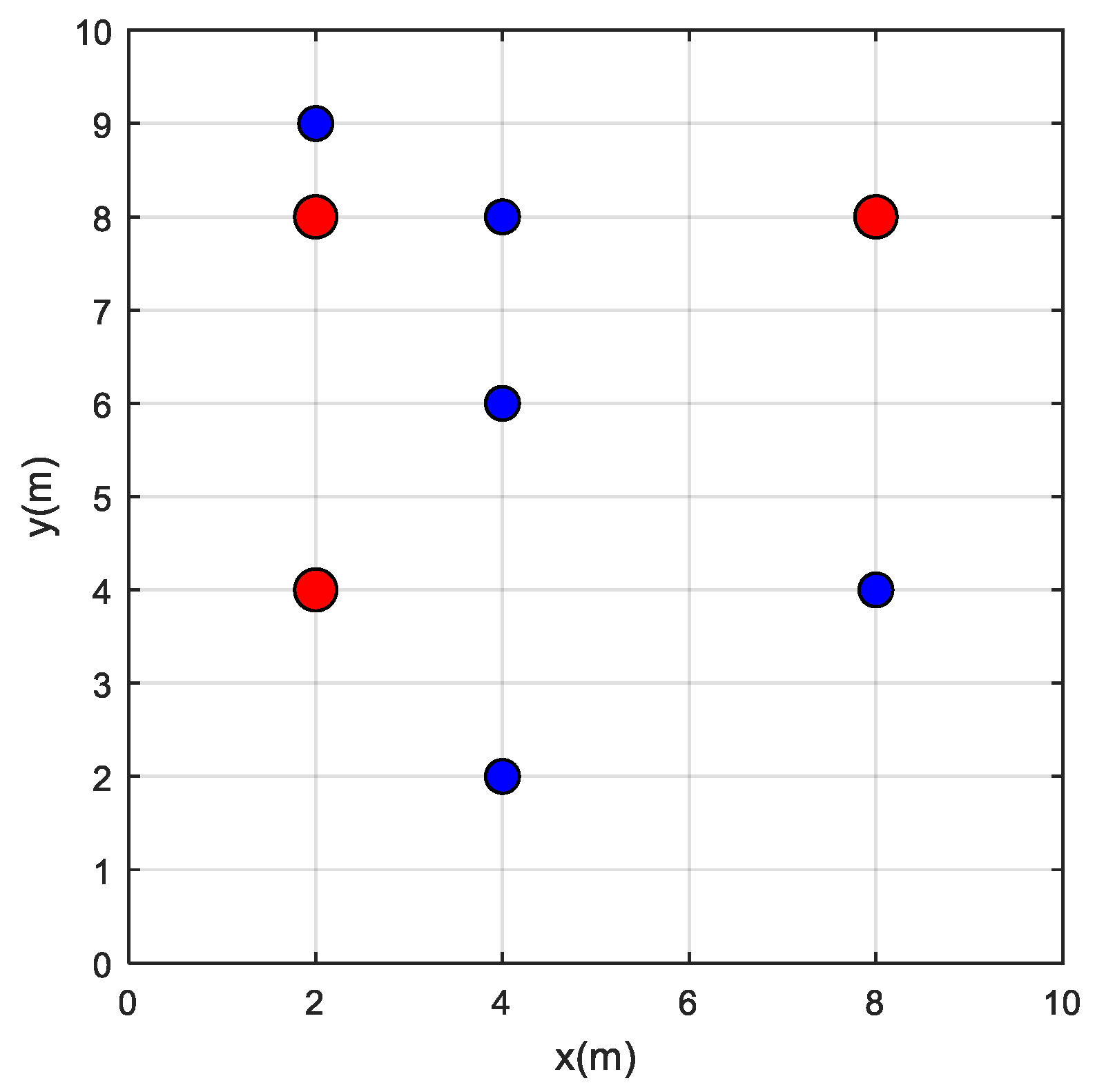
Let us assume that we have three reference nodes located at (2,4), (8,8), and (2,8) along with five target nodes located at (4,2), (8,4), (4,6), (4,8), and (2,9) as shown in Figure 2. Using the proposed approach first the distances between reference nodes and target nodes are estimated as follows:
DistanceRT = [ d 11 d 12 d 13 d 14 d 15 d 21 d 22 d 23 d 24 d 25 d 31 d 32 d 33 d 34 d 35 ]
which is numerically given by:
DistanceRT = [ 2.8284 6.0000 2.8284 4.4721 5.0000 7.2111 4.0000 4.4721 4.0000 6.0828 6.3246 7.2111 2.8284 2.0000 1.0000 ]
As explained before, in this subsection we assume that these distances are estimated using RSSI.
Then the MVPA solves the optimization problem to calculate ( x 1 , y 1 ) ,   ( x 2 , y 2 ) ,   ( x 3 , y 3 ) , ( x 4 , y 4 ) , and ( x 5 , y 5 ) while minimizing the objective function given by Equation (7). The results (i.e., the coordinates ( x i , y i ) ) along with the mean squared errors (MSE) obtained using MVPA and the other five algorithms are tabulated in Table 1. It can be seen from this table that the MVPA along with the SQP were able to calculate the actual coordinates of all target nodes with an accuracy of less than 5 cm (tolerance on estimation error). However, all the remaining algorithms have found some difficulties and made some mistakes to calculate the coordinates of the target nodes as highlighted in soft red in Table 1. The evolution of the objective function is sketched in Figure 3. It can be seen from this figure that the MVPA has the best convergence among all other algorithms.

3.1.2. Case 2

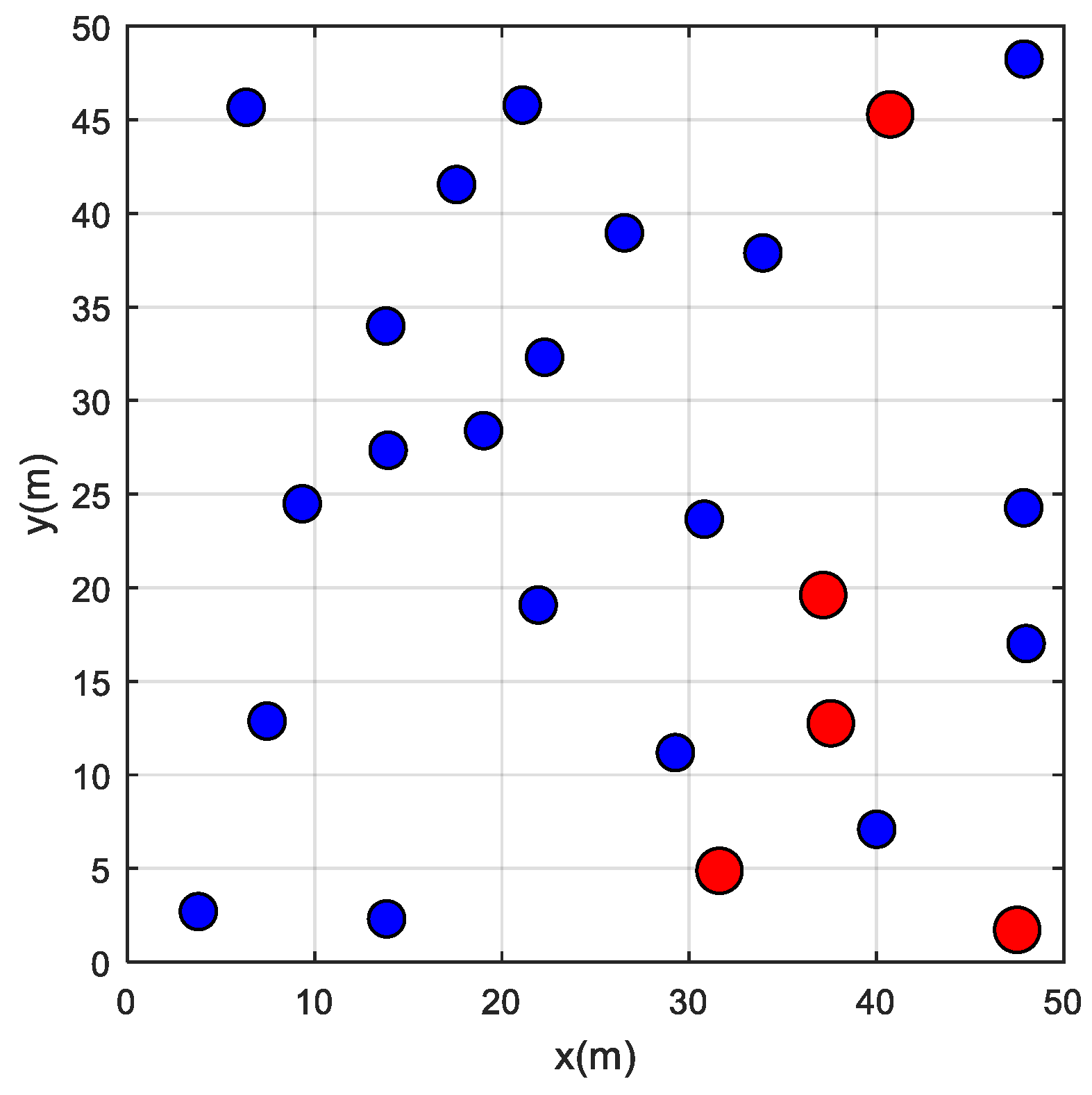
In this case, 25 nodes are generated randomly in a given space of 50 m × 50 m among these 25 nodes, 5 nodes are considered as reference nodes (i.e., their location is known and the distances from these nodes to the remaining target nodes are also known). This case is represented in Figure 4, where red and blue circles represent reference and target nodes, respectively.
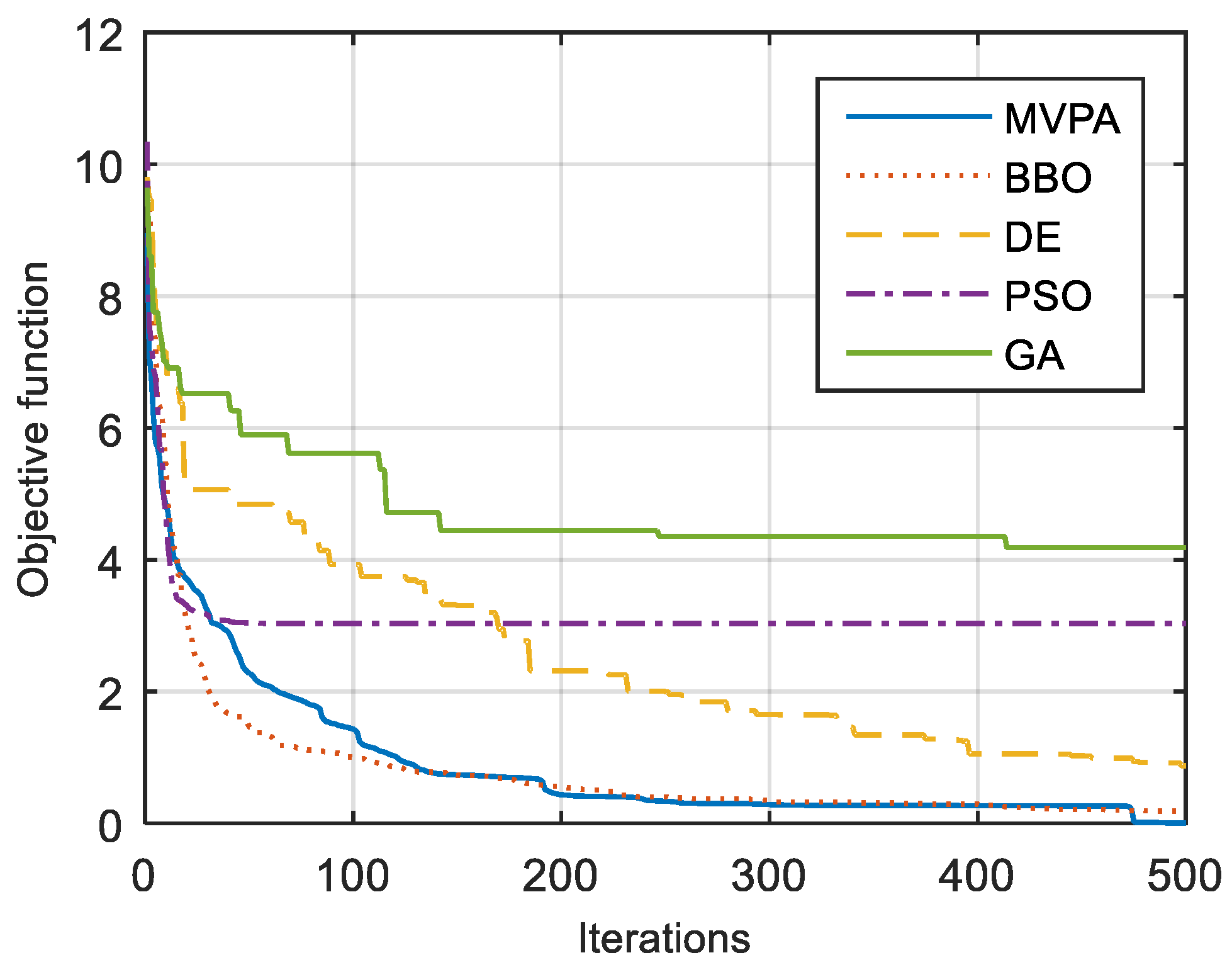
The obtained results along with the MSE for this case are tabulated in Table 2. From this table, the proposed approach using the MVPA was able to find all the locations of target nodes within a small range compared with the actual coordinates. However, the remaining algorithms have struggled to find the desired locations as highlighted in the table. From the curves plotted in Figure 5, it can be noticed that the MVPA converges to the lowest value of the objective function.

3.1.3. Case 3

In this case, the number of nodes is increased to 50. Among these nodes, 10 nodes are considered reference nodes. This case is represented in Figure 6.
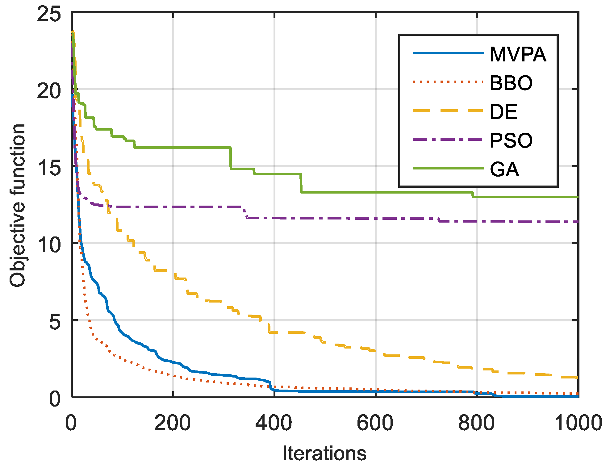
The obtained results along with the MSE for this case are tabulated in Table 3. It can be seen from this table that the MVPA was able to find the coordinates of all target points with good accuracy (less than 5 cm) except for two locations; at the same time, the remaining algorithms have struggled to do so. Moreover, the objective function minimized over the iterations is sketched in Figure 7.

3.1.4. Case 4

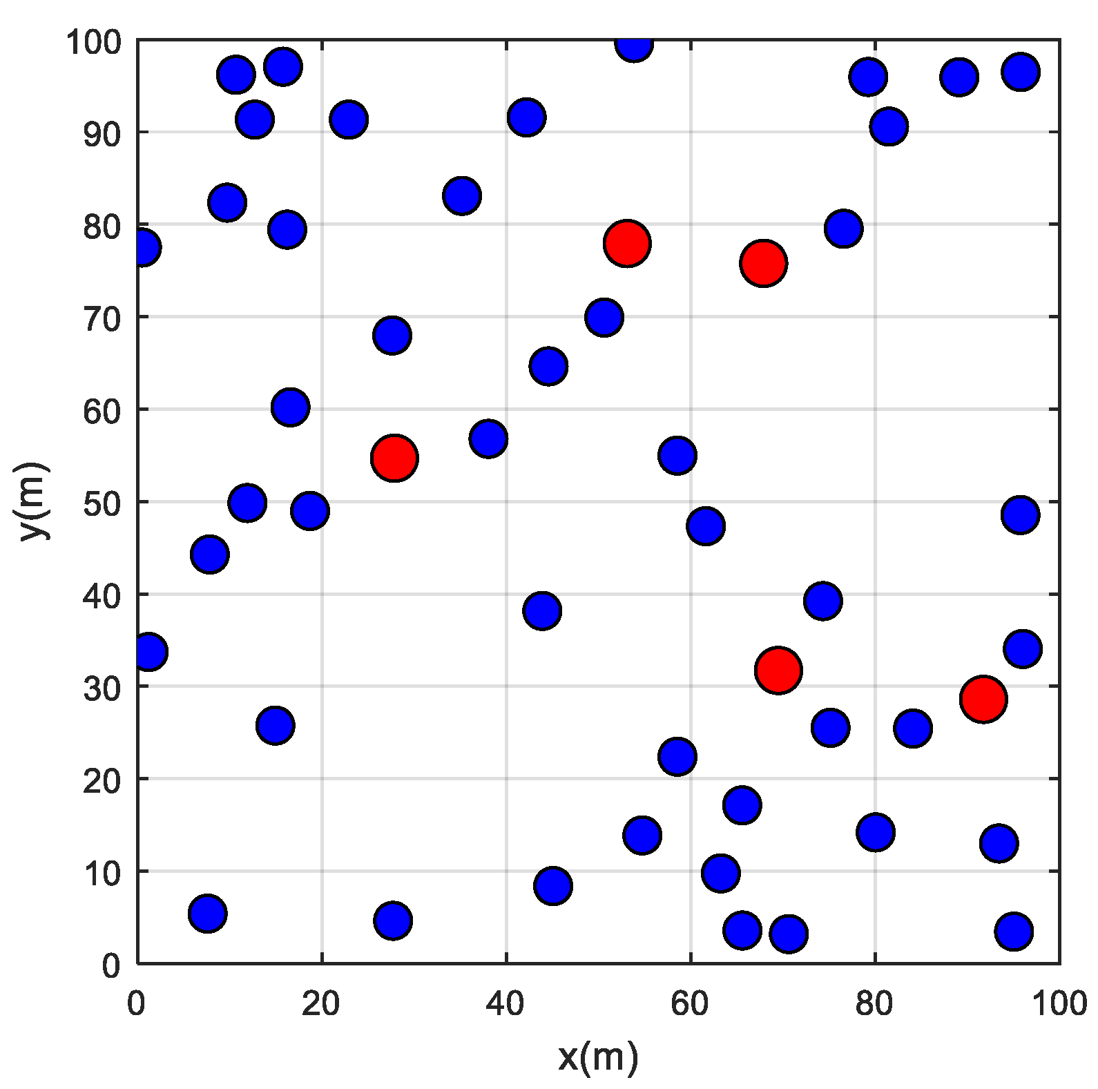
In this case, the number of nodes is 50 nodes in a space of 100 m × 100 m. Among these nodes, 5 nodes only are considered as reference nodes. This case is represented in Figure 8. Compared to the previous case a smaller number of reference nodes and a wider space are considered here. This will test the efficiency and robustness of the MVPA.
This case, which is the hardest case to solve because of the low number of reference points and the high number of target points, is solved using MVPA and the results are tabulated in Table 4. It can be seen that the MVPA is by far the best algorithm in estimating the coordinates of target nodes compared to the remaining algorithms. It has estimated five nodes with less accuracy than 5 cm whereas other algorithms have shown low accuracy for most of the cases, or rather have wrongly estimated the location of a few nodes. The curves of the evolution of the objective function are sketched in Figure 9.
Looking at Figure 5, Figure 7 and Figure 9, it can be noticed that although the BBO has a quick speed of convergence, the MVPA converges to a better final solution. This statement is confirmed by the results tabulated in Table 1, Table 2 and Table 3 where the MSEs obtained using MVPA are lower than the ones obtained using all the comparing algorithms including the BBO in all cases.

3.2. B. Real-Time Experimental Study

In [23] a real wireless network with three reference nodes and one target node (that can be moved to have multiple measurements) were studied. The target node and reference nodes are created using Zigbee series two modules, that were chosen for being less expensive and power-efficient [37,38]. As aforesaid, the reference nodes are acting as three routers whereas the target node acts as a device that receives signals from three transmitting devices (reference nodes) at any instant. A local coordinate system was established such that both x and y coordinates increase by half feet i.e., each integer in the coordinate system is representative of two feet (0.6096 m). The coordinates of the three reference nodes on a local coordinate system are (0,0), (6,0), and (3,8) for both indoor and outdoor settings as shown in [23].
The target node was relocated to ten independent positions as shown by the blue dots in Figure 10. The coordinates of these nodes along with the distances measured between reference nodes and target nodes, in meters, are tabulated in Table 5. The last column gives the average of the distances of the target node from all three nodes.

3.2.1. Distance Estimation Based on Measured RSSI

As aforesaid, to determine the coordinates of a real system, first, the distances are estimated from the measured RSSI using a nonlinear regression model and approximating that model on LNSM of Equation (3). Then the proposed MVPA is run to localize the coordinates of the local grid. RSSI is measured for each of the ten locations of the target node using range testing of the XCTU software (XCTU offers a convenient graphical interface where developers can deal with multiple Digi RF modules simultaneously. It is available in several platforms as an open-source application) [39]. The coordinates of the ten locations where the target node is kept are given in the first column of Table 5. At each location, ten values of RSSI are noted and their average RSSI is computed. The average RSSI of each location for both indoor and outdoor settings is shown in Figure 11. It can be noted that as the target node is moved far away from a specific reference node, the received RSSI is decreased. Moreover, the signal strength observed in the outdoor environment is less than that observed in the indoors. Based on these measurements, a nonlinear regression model is developed to estimate the distances from measured RSSI.
The relationship between RSSI and distance obtained using our nonlinear regression model for indoor experiments is expressed as follows:
R S S I = 23.671 18.78 × l o g ( d )
and therefore:
d = 10 R S S I + 23.671 18.78
The relationship between RSSI and distance obtained using our model for outdoor experiments is expressed as follows:
R S S I = 40.425 10.10 × l o g ( d )
and therefore:
d = 10 R S S I + 40.425 10.10
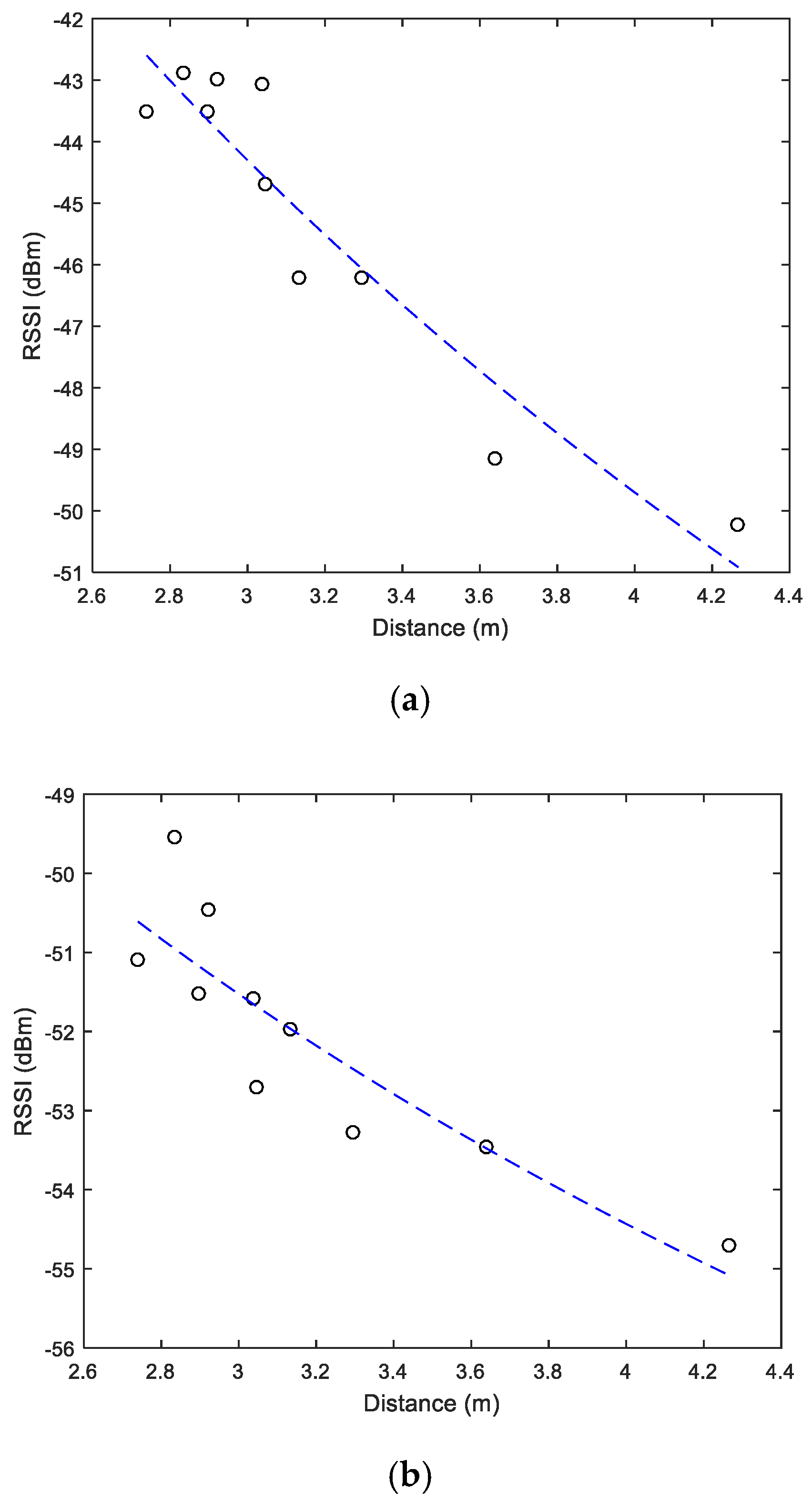
Comparing (10) and (12) with (3) reveals that the terms P t P L ( d 0 ) + X σ is equal to −23.671 (dBm) for the indoor case and −40.425 (dBm) for the outdoor case. However, the value of 10   n log 10 can be approximated to −18.78 (dBm) and −10.10 (dBm) for indoor and outdoor scenarios, respectively. Equations (10) and (12) are plotted in Figure 12a,b, respectively. It can be seen that the nonlinear curves approximate the best function such that the error function between the measured values and the approximated curve is minimized.

3.2.2. Coordinate Estimation Using MVPA

The distances estimated in the previous section for outdoor application are given to the MVPA algorithm to determine the coordinates of the target nodes. The results are displayed in Table 6. It can be seen from this table that the locations are well estimated, and the error is mainly due to the estimation of the distances from RSSI using the nonlinear regression model.

4. Conclusions

Localization of sensor nodes has always intrigued wireless network engineers as it enables them to deploy efficient network protocols and minimize the traffic and hence the latency on a given channel. To realize the effective and accurate localization, this paper has effectively demonstrated the two-fold technique toward localization; first, a nonlinear regression model is used to establish an approximate relationship between RSSI and distance between the sensors, later, those distances are fed to MVPA to figure out the geometrical coordinates in the local 2d space. The model is first implemented on four simulation-based test cases, where the results obtained from MVPA are compared with the contemporary techniques for benchmarking. Finally, the applicability of the proposed method is demonstrated on actual WSN in both indoor and outdoor environments. It is found that the proposed MVPA estimation method preceded by nonlinear regression has given good results for distance estimation and node localization. The approach is tested under rigorous simulation scenarios spanning a large area and equipped with a very low number of reference nodes. Even in the most constrained problem (case 4), the MSE in the x-coordinate of the proposed approach is 24 times less than the second-best approach (BBO). Similarly, for the y-coordinate, the MSE obtained with the proposed MVPA is 20 times less than that of the BBO approach, the second-best performer. Future directions can focus more on how to improve the estimation of distances based on RSSI using regression models or even Artificial Neural Networks (ANNs). Another future work can also be to test the developed approach for a network with obstacles like walls for example.

Author Contributions

Formal analysis, H.R.E.H.B.; Funding acquisition, M.A.A.; Methodology, H.R.E.H.B. and M.S.J.; Software, H.R.E.H.B.; Supervision, M.A.A.; Writing—original draft, M.A.A.; Writing—review & editing, H.R.E.H.B. and M.S.J. All authors have read and agreed to the published version of the manuscript.

Funding

This research was funded by the Deanship of Scientific Research, University of Hafr Al Batin, grant number G-101-2020.

Institutional Review Board Statement

Not applicable.

Informed Consent Statement

Not applicable.

Data Availability Statement

Not applicable.

Acknowledgments

The authors extend their appreciation to the Deanship of Scientific Research, University of Hafr Al Batin, for funding this work through the research group project No G-101-2020.

Conflicts of Interest

The authors declare no conflict of interest.

References

  1. Kanoun, O.; Bradai, S.; Khriji, S.; Bouattour, G.; El Houssaini, D.; Ben Ammar, M.; Naifar, S.; Bouhamed, A.; Derbel, F.; Viehweger, C. Energy-aware system design for autonomous wireless sensor nodes: A comprehensive review. Sensors 2021, 21, 548. [Google Scholar] [CrossRef] [PubMed]
  2. Martin, S. Internet of Things Learning and Teaching. Technologies 2021, 9, 7. [Google Scholar] [CrossRef]
  3. De Nardis, L.; Caso, G.; Benedetto, M.G. Di ThingsLocate: A ThingSpeak-Based Indoor Positioning Platform for Academic Research on Location-Aware Internet of Things. Technologies 2019, 7, 50. [Google Scholar] [CrossRef] [Green Version]
  4. Potdar, V.; Sharif, A.; Chang, E. Wireless sensor networks: A survey. In Proceedings of the International Conference on Advanced Information Networking and Applications, AINA, Bradford, UK, 26–29 May 2009; pp. 636–641. [Google Scholar]
  5. Ahmadi, Y.; Neda, N.; Ghazizadeh, R. Range Free Localization in Wireless Sensor Networks for Homogeneous and Non-Homogeneous Environment. IEEE Sens. J. 2016, 16, 8018–8026. [Google Scholar] [CrossRef]
  6. Fang, X.; Nan, L.; Jiang, Z.; Chen, L. Multi-channel fingerprint localisation algorithm for wireless sensor network in multipath environment. IET Commun. 2017, 11, 2253–2260. [Google Scholar] [CrossRef]
  7. Obeidat, H.A.; Dama, Y.A.S.; Abd-Alhameed, R.A.; Hu, Y.F.; Qahwaji, R.; Noras, J.M.; Jones, S.M.R. A comparison between vector algorithm and CRSS algorithms for indoor localization using received signal strength. Appl. Comput. Electromagn. Soc. J. 2016, 31, 868–876. [Google Scholar]
  8. Wang, X.; Xu, P.; Xue, W. Research on online signal matching of indoor positioning based on AL-KNN algorithm. In Proceedings of the 2017 International Applied Computational Electromagnetics Society Symposium in China (ACES-China 2017), Suzhou, China, 1–4 August 2017. [Google Scholar]
  9. Drawil, N.M.; Amar, H.M.; Basir, O.A. GPS localization accuracy classification: A context-based approach. IEEE Trans. Intell. Transp. Syst. 2013, 14, 262–273. [Google Scholar] [CrossRef]
  10. Zhang, Y.; Wu, W.; Chen, Y. A Range-Based Localization Algorithm for Wireless Sensor Networks. J. Commun. Netw. 2005, 7, 429–437. [Google Scholar] [CrossRef]
  11. Xiong, H.; Chen, Z.; Yang, B.; Ni, R. TDOA localization algorithm with compensation of clock offset for wireless sensor networks. China Commun. 2015, 12, 193–201. [Google Scholar] [CrossRef]
  12. Shen, H.; Ding, Z.; Dasgupta, S.; Zhao, C. Multiple source localization in wireless sensor networks based on time of arrival measurement. IEEE Trans. Signal Process. 2014, 62, 1938–1949. [Google Scholar] [CrossRef]
  13. Sheng, X.; Hu, Y.H. Maximum likelihood multiple-source localization using acoustic energy measurements with wireless sensor networks. IEEE Trans. Signal Process. 2005, 53, 44–53. [Google Scholar] [CrossRef] [Green Version]
  14. Malajner, M.; Gleich, D.; Planinšič, P. Angle of arrival measurement using multiple static monopole antennas. IEEE Sens. J. 2015, 15, 3328–3337. [Google Scholar] [CrossRef]
  15. Mardini, W.; Khamayseh, Y.; Almodawar, A.A.; Elmallah, E. Adaptive RSSI-based localization scheme for wireless sensor networks. Peer-to-Peer Netw. Appl. 2016, 9, 991–1004. [Google Scholar] [CrossRef]
  16. Trueman, C.W.; Davis, D.; Segal, B. Relationship between the path loss exponent and the room absorption for line-of-sight communication. Appl. Comput. Electromagn. Soc. J. 2009, 24, 361–367. [Google Scholar]
  17. Kurt, S.; Tavli, B. Path-Loss Modeling for Wireless Sensor Networks: A review of models and comparative evaluations. IEEE Antennas Propag. Mag. 2017, 59, 18–37. [Google Scholar] [CrossRef]
  18. Meenalochani, M.; Sudha, S. Fuzzy based estimation of received signal strength in a wireless sensor network. In Proceedings of the ACM International Conference Proceeding Series; Association for Computing Machinery: New York, NY, USA, 2015; pp. 624–628. [Google Scholar]
  19. Meenalochani, M.; Sudha, S. Jammed Node Detection and Routing in a Multihop Wireless Sensor Network Using Hybrid Techniques. Wirel. Pers. Commun. 2019, 104, 663–675. [Google Scholar] [CrossRef]
  20. MakalYucedag, S.; Kizilay, A. Time domain analysis of ultra-wide band signals from buried objects under flat and slightly rough surfaces. Appl. Comput. Electromagn. Soc. J. 2013, 28, 646–652. [Google Scholar]
  21. Al Sayyari, A.; Kostanic, I.; Otero, C.E. An empirical path loss model for Wireless Sensor Network deployment in a concrete surface environment. In Proceedings of the IEEE 16th Annual Wireless and Microwave Technology Conference, WAMICON 2015, Cocoa Beach, FL, USA, 13–15 April 2015; Institute of Electrical and Electronics Engineers Inc.: New York, NY, USA, 2015. [Google Scholar]
  22. Passafiume, M.; Maddio, S.; Lucarelli, M.; Cidronali, A. An enhanced triangulation algorithm for a distributed RSSI-DoA positioning system. In Proceedings of the 13th European Radar Conference, EuRAD, London, UK, 5–7 October 2016; pp. 185–188. [Google Scholar]
  23. Manickam, M.; Selvaraj, S. Range-based localisation of a wireless sensor network using Jaya algorithm. IET Sci. Meas. Technol. 2019, 13, 937–943. [Google Scholar] [CrossRef]
  24. Bouchekara, H.R.E.H. Most Valuable Player Algorithm: A novel optimization algorithm inspired from sport. Oper. Res. 2020, 20, 139–195. [Google Scholar] [CrossRef]
  25. Alatas, B. Sports inspired computational intelligence algorithms for global optimization. Artif. Intell. Rev. 2017. [Google Scholar] [CrossRef]
  26. Ouili, M.; Mehasni, R.; Feliachi, M.; Allag, H.; Bouchekara, H.R.E.H.; Berthiau, G.; Latreche, M.E.H. Coupling of 3D analytical calculation and PSO for the identification of magnet parameters used in magnetic separation. Appl. Comput. Electromagn. Soc. J. 2019, 34, 1607–1615. [Google Scholar]
  27. Ramli, M.A.M.; Bouchekara, H.R.E.H. Efficient Energy Management in a Microgrid with Intermittent Renewable Energy and Storage Sources. Sustainability 2019, 11, 3839. [Google Scholar] [CrossRef] [Green Version]
  28. Korashy, A.; Kamel, S.; Youssef, A.R.; Jurado, F. Most Valuable Player Algorithm for Solving Direction Overcurrent Relays Coordination Problem. In Proceedings of the International Conference on Innovative Trends in Computer Engineering, ITCE 2019, Aswan, Egypt, 2–4 February 2019; Institute of Electrical and Electronics Engineers Inc.: New York, NY, USA, 2019; pp. 466–471. [Google Scholar]
  29. Ramli, M.A.M.; Bouchekara, H.R.E.H. Wind Farm Layout Optimization Considering Obstacles Using a Binary Most Valuable Player Algorithm. IEEE Access 2020, 8, 131553–131564. [Google Scholar] [CrossRef]
  30. Liu, X.; Luo, Q.; Wang, D.; Abdel-Baset, M.; Jiang, S. An improved most valuable player algorithm with twice training mechanism. In Proceedings of the Lecture Notes in Computer Science (Including Subseries Lecture Notes in Artificial Intelligence and Lecture Notes in Bioinformatics); Springer: Berlin/Heidelberg, Germany, 2018; Volume 10954, LNCS; pp. 854–865. [Google Scholar]
  31. Srilakshmi, K.; Ravi Babu, P.; Aravindhababu, P. An enhanced most valuable player algorithm based optimal power flow using Broyden’s method. Sustain. Energy Technol. Assess. 2020, 42, 100801. [Google Scholar] [CrossRef]
  32. Eberhart, R.; Kennedy, J. A new optimizer using particle swarm theory. In Proceedings of the Sixth International Symposium on Micro Machine and Human Science, Nagoya, Japan, 4–6 October 1995; pp. 39–43. [Google Scholar]
  33. Kennedy, J.; Eberhart, R. Particle swarm optimization. Neural Netw. 1995 Proc. IEEE Int. Conf. 1995, 4, 1942–1948. [Google Scholar] [CrossRef]
  34. Storn, R.; Price, K. Differential Evolution—A Simple and Efficient Heuristic for global Optimization over Continuous Spaces. J. Glob. Optim. 1997, 11, 341–359. [Google Scholar] [CrossRef]
  35. Qing, A. DIFFERENTIAL EVOLUTION Fundamentals Fundamentals and Applications in Electrical Engineering; John Wiley & Sons: Hoboken, NJ, USA, 2009; ISBN 9780470823927. [Google Scholar]
  36. Simon, D.; Member, S. Biogeography-Based Optimization. IEEE Trans. Evol. Comput. 2008, 12, 702–713. [Google Scholar] [CrossRef] [Green Version]
  37. Natarajan, H.; Nagpal, S.K.; Selvaraj, S. Impact of rate of recurrent communication of sensor node on network lifetime in a wireless sensor network. IET Sci. Meas. Technol. 2017, 11, 473–479. [Google Scholar] [CrossRef]
  38. Uma Maheswari, D.; Meenalochani, M.; Sudha, S. Influence of the cluster head position on the lifetime of wireless sensor network—A case study. In Proceedings of the 2016 2nd International Conference on Next Generation Computing Technologies, NGCT 2016, Dehradun, India, 14–16 October 2016; Institute of Electrical and Electronics Engineers Inc.: New York, NY, USA, 2017; pp. 378–381. [Google Scholar]
  39. XCTU—Download and Install the Configuration Platform for XBee/RF Solutions|Digi International. Available online: https://www.digi.com/products/embedded-systems/digi-xbee/digi-xbee-tools/xctu (accessed on 23 March 2021).
Figure 1. Flowchart of the proposed approach.
Technologies 09 00042 g001
Figure 2. Plot of reference and target nodes for case 1.
Technologies 09 00042 g002
Figure 3. Evolution of the objective function versus iterations for case 1.
Technologies 09 00042 g003
Figure 4. Plot of reference and target nodes for case 2.
Technologies 09 00042 g004
Figure 5. Evolution of the objective function versus iterations for case 2.
Technologies 09 00042 g005
Figure 6. Plot of reference and target nodes for case 3.
Technologies 09 00042 g006
Figure 7. Evolution of the objective function versus iterations for case 3.
Technologies 09 00042 g007
Figure 8. Plot of reference and target nodes for case 4.
Technologies 09 00042 g008
Figure 9. Evolution of the objective function versus iterations for case 4.
Technologies 09 00042 g009
Figure 10. Plot of reference and target nodes for real-time experimental study.
Technologies 09 00042 g010
Figure 11. Average measured RSSI for (a) indoor experiments, and (b) outdoor experiments at ten different locations of target nodes.
Technologies 09 00042 g011
Figure 12. Nonlinear regression estimation of the relationship between the measured RSSI and the distance d: (a) indoor scenario, (b) outdoor scenario.
Technologies 09 00042 g012
Table 1. Comparison of actual locations with those obtained using different algorithms for case 1.
Actual ValuesMVPABBODEPSOGASQP
xiyixiyixiyixiyixiyixiyixiyi
4.0002.0004.0002.0004.0372.0173.9401.9754.0032.0033.1571.43942
8.0004.0008.0004.0008.0114.0187.9993.9948.0003.9998.1543.5607.9994
4.0006.0004.0006.0004.0455.9264.0366.0184.0055.9993.9196.28946
4.0008.0004.0008.0004.0247.9484.0158.1344.0137.9943.9738.05848
2.0009.0002.0009.0001.9869.0051.9979.0032.0039.0001.9718.97528.999
MSE008.57 × 10−41.76 × 10−31.03 × 10−33.79 × 10−34.24 × 10−59.40 × 10−61.48 × 10−11.19 × 10−12.00 × 10−72.00 × 10⁻⁷
Table 2. Comparison of actual locations with those obtained using different algorithms for case 2.
Actual ValuesMVPABBODEPSOGASQP
xiyixiyixiyixiyixiyixiyixiyi
6.34945.6696.34945.6717.09146.3515.52344.8336.94550.0006.35947.6946.35045.669
13.92527.34413.93027.34414.53028.20714.68927.70914.64528.68512.27026.93813.92427.343
47.87548.24447.87648.24547.83648.30149.99047.27530.62750.00034.78439.83236.59350.000
47.85824.26947.86024.26447.77524.33547.65325.33846.67625.22633.00224.64529.68526.043
40.0147.09440.0117.09439.9667.07340.6765.75340.1947.82732.9765.54840.0157.094
21.08845.78721.08045.78222.82146.60922.21346.33027.87650.0005.23530.94421.08945.787
33.93737.88733.93737.88733.92238.04541.18836.00531.26037.61444.70739.15833.93637.887
13.8462.30913.8492.30514.0721.92614.2850.11114.2432.0647.9986.72813.8462.309
21.93719.07821.93819.07922.22919.44321.11316.79320.83313.98926.60514.34321.93719.078
9.34424.4889.34424.4889.02823.7269.54924.52310.64833.10410.28830.1019.34424.489
22.27932.31622.30532.33822.53632.51724.40333.21130.40331.89841.61640.00822.27932.316
13.80133.98513.80033.98412.46132.20314.29434.22525.04942.02946.17337.87713.80233.985
47.98717.01947.98917.01748.03917.02348.14615.52947.94016.86440.02825.44128.16018.953
29.26311.19129.26311.18928.94811.19227.18010.61027.12010.43830.83017.43129.26311.191
7.46512.8757.46512.8687.49812.8226.89112.2543.2550.0009.35618.1837.46412.874
30.80223.66430.80323.66530.53923.32529.28825.26929.2872.96331.76523.71630.80123.664
17.58341.54117.58541.54417.54941.47817.30240.80118.89042.36420.67345.15417.58441.543
19.02228.39119.01828.38618.74228.14019.11728.74549.26034.18123.3889.76319.02328.392
3.7932.6983.7932.6983.7822.7494.8790.50713.09638.4144.87513.2653.7932.697
26.54038.95826.53838.95827.67039.57249.63438.54825.87538.81519.97840.50326.54038.958
MSE4.09 × 10−53.24 × 10−53.78 × 10−13.28 × 10−13.04 × 1011.53 × 1007.88 × 1011.06 × 1021.22 × 1025.30 × 1014.25 × 1014.99 × 10−1
Table 3. Comparison of actual locations with those obtained using different algorithms for case 3.
Actual ValuesMVPABBODEPSOGASQP
xiyixiyixiyixiyixiyixiyixiyi
12.69991.33812.69991.33712.24691.45223.45099.89867.81943.36757.19480.89916.67592.279
95.75196.48995.75296.48695.66496.74293.67297.088100.000100.00085.41195.00095.79296.220
95.71748.53895.71548.54094.63348.94397.96552.15651.64452.11089.65165.93795.73748.586
80.02814.18980.02814.18980.06913.72379.09915.970100.00047.66289.1236.79980.20214.176
42.17691.57442.17591.57441.93992.43341.44292.775100.00041.65431.68568.36542.15091.550
65.5743.57165.5753.57265.4383.08263.7022.17761.9990.00066.8420.41562.9782.757
67.87475.77467.87375.77567.91575.96671.35874.33960.89776.54770.11872.70668.09475.754
74.31339.22374.31339.22375.28039.20874.54040.22965.80722.72558.64744.44574.25239.262
65.54817.11965.55017.12165.00116.97565.12015.41365.51517.19348.74271.54365.51217.145
27.6924.61727.6924.61727.5344.62928.3391.92859.9210.0003.99843.96428.0824.633
9.71382.3469.71182.34410.72683.29312.35982.81929.18991.25112.53788.11517.07186.644
69.48331.71069.48331.71069.29231.67470.39433.25668.52435.60469.69431.37169.44031.672
95.0223.44595.0343.48394.6552.86699.9877.60792.2160.00092.9057.71394.8213.388
43.87438.15643.87438.15544.79338.66042.80038.00057.79138.89719.50377.19243.86738.253
76.55279.52076.55479.51676.30879.66676.06678.94979.42878.9659.71761.03376.49579.615
18.68748.97618.67249.01219.15348.74316.73853.31447.19358.48443.77237.00218.95049.336
44.55964.63144.56064.63244.65564.69044.22263.58758.42061.33032.09358.52044.57164.656
11.90049.83611.90049.83611.63350.09015.38749.3370.00057.19511.23464.01812.04949.839
95.97434.03995.97434.03895.95934.11895.98834.809100.00037.35697.44724.45496.16334.481
58.52722.38158.53422.38958.45422.41558.04123.65954.76422.78022.0655.48158.34622.385
75.12725.51075.12725.51075.42025.54574.00726.87643.2320.00033.38729.32375.16025.526
50.59669.90850.59969.90350.50369.80651.75269.65979.47165.57471.48465.65250.57069.776
89.09095.92988.14897.00089.14395.62489.72694.80535.52794.50192.34390.43189.39195.651
54.72213.86254.75413.86854.16212.97555.11116.91139.09037.98864.89422.50754.55513.689
14.92925.75114.92925.75114.96025.74713.93424.0610.00039.28149.90619.33012.04725.429
61.60447.32961.60547.33061.71747.45860.61945.89735.65731.42735.19615.72062.12947.431
35.16683.08335.16783.08335.13683.10536.56582.9580.00072.83032.12387.21835.14583.190
58.52654.97258.52654.97258.37354.84857.53554.15762.38453.59247.00161.16958.58454.990
91.71928.58491.72028.58591.95628.85091.22728.12473.5547.75893.6844.16491.75328.489
53.08077.91753.08077.91752.83577.84651.84676.636100.00076.68153.33982.26353.08677.841
93.40112.99193.40712.99992.87812.24792.44413.87836.0410.00079.69350.30093.36212.859
1.19033.7121.19033.7161.04634.1201.84932.6221.99531.36735.91715.56611.96521.770
16.21879.42816.20879.41916.17379.43716.01680.13017.97780.55212.99645.99515.08178.974
16.56560.19816.56560.19816.65860.21317.54165.07122.56953.92425.30442.15316.48460.225
45.0548.38245.0558.38245.1868.46144.5308.66245.77111.92782.18824.60745.0008.379
22.89891.33422.90691.33822.28991.14328.24992.90928.479100.00042.46193.58120.23290.099
53.83499.61353.83499.61454.35499.31853.78499.94780.08161.97438.18984.21153.78299.364
7.81844.2687.81744.2688.03944.1167.56944.69626.86136.81118.12932.1777.78744.177
10.66596.19010.44595.95910.94696.4879.95496.05710.633100.00021.21090.46846.63196.050
0.46377.4910.46377.4911.44778.7250.04577.86038.54794.2395.97295.55240.01584.358
MSE2.34 × 10−23.01 × 10−21.94 × 10−11.65 × 10−15.87 × 1004.96 × 1006.80 × 1022.71 × 1024.67 × 1023.57 × 1027.67 × 1015.31 × 100
Table 4. Comparison of actual locations with those obtained using different algorithms for case 4.
Actual ValuesMVPABBODEPSOGASQP
xiyixiyixiyixiyixiyixiyixiyi
81.47290.57981.47290.57981.62290.43578.37890.22481.689100.00084.55883.65647.89483.877
12.69991.33812.61991.29312.99291.43910.42388.99912.85793.49122.66184.0890.00036.845
63.2369.75463.2339.75462.7759.72163.37410.43783.68012.55790.61310.38562.59910.597
95.75196.48996.35195.71895.60396.00993.46598.841100.00092.9894.75532.92324.27941.997
15.76197.05915.73197.03117.06098.20816.15496.48415.71897.98612.68323.4940.00036.888
95.71748.53895.71848.53895.94648.80096.29346.62369.86321.99167.34716.97978.48629.237
80.02814.18980.06714.20579.64814.265100.00022.88787.65121.46757.24918.00780.71214.171
42.17691.57441.10290.64243.03792.09639.90689.19840.12988.43430.51887.64641.98191.744
79.22195.94979.19695.98279.14495.93783.06692.96885.62596.82797.57896.87343.69989.282
65.5743.57165.5503.57265.7653.32761.2353.108100.0000.24968.70416.58869.0843.359
74.31339.22374.32839.25374.78839.84971.35934.31972.18747.57275.75553.11174.50239.160
65.54817.11965.54217.11865.82616.98966.73616.30965.51612.78245.03727.52365.97917.160
70.6053.18370.6133.18371.1023.32068.2690.00076.4850.00075.20320.14376.1925.046
27.6924.61727.6924.61727.9904.38429.5231.29827.5874.12729.08533.03127.1355.203
9.71382.3469.71382.3459.68182.3751.32276.77715.949100.00026.71430.5030.00036.932
95.0223.44595.0193.44393.3082.26890.0110.27590.9940.81359.7604.88178.9490.000
43.87438.15643.87138.15643.39938.40244.01337.63735.49735.55837.92337.12744.79538.240
76.55279.52076.55179.52076.35880.12273.57681.11034.532100.00063.85381.34776.77779.106
18.68748.97618.70148.95418.39248.93523.81663.07323.75389.43656.00263.90216.98552.233
44.55964.63144.55464.63244.44464.92642.64062.85148.07368.04150.11767.70144.62664.077
27.60367.97027.60067.97027.48767.90428.05269.19314.13055.49533.65476.06827.98367.478
11.90049.83611.89649.84912.18549.24012.37951.19813.82757.34926.95839.96911.84349.967
95.97434.03995.97634.04095.48433.50299.98538.5170.00035.95880.46423.02095.94333.456
58.52722.38158.52722.38057.88221.98663.99922.29089.09744.73571.5278.22958.35422.686
75.12725.51075.16125.52476.13626.47872.35324.298100.00043.71394.90530.35074.81225.280
50.59669.90850.59669.90850.92669.32149.19772.39249.71376.37873.98067.51250.59470.075
89.09095.92989.08495.93188.20097.09583.61698.416100.00069.95090.88192.39536.54480.275
54.72213.86254.71813.87054.76213.85554.35613.657100.00026.89069.77530.51254.27613.648
14.92925.75114.92925.75117.49323.74112.51929.02080.3730.00027.67551.52715.46725.731
84.07225.42884.07225.42985.00926.07486.79027.91389.7679.53443.84547.37684.93426.552
61.60447.32961.57247.27661.69847.26563.37648.68889.39892.89071.80159.93958.60743.789
35.16683.08335.16683.08235.46882.77834.33484.19313.74443.54634.85685.71335.20283.401
58.52654.97258.52754.97257.83955.06556.64253.50086.71377.64949.64223.49457.93254.584
38.04556.78238.04856.78337.31257.21937.61457.23844.18661.74743.85756.73337.84158.355
7.5855.3957.5885.3896.8525.8031.02311.5944.3670.00032.94694.8799.1413.298
93.40112.99193.38512.98195.15613.44591.98514.383100.00022.19099.1745.44379.4414.864
1.19033.7121.18133.7241.23334.0750.38334.81525.7630.0019.03594.6111.42035.517
16.21879.42816.21979.43315.71279.06113.91177.42215.108100.00051.58563.7726.81154.286
16.56560.19816.56160.19016.34660.40014.96957.77018.73275.76179.24990.30716.24560.869
45.0548.38245.0358.38445.7448.02948.3849.4655.48928.39545.19714.29645.4108.065
22.89891.33422.89891.33422.53791.20231.659100.00016.56574.06046.1484.89111.28758.981
53.83499.61353.71999.54751.64898.46552.62299.23024.00770.40643.74584.85448.62996.527
7.81844.2687.82344.2567.64144.7770.00057.01717.19335.97213.08031.0526.09546.505
10.66596.19010.66596.1908.03593.55415.12599.74313.075100.00011.81850.9610.00236.758
0.46377.4910.46577.4962.01780.34317.21399.9320.0000.00025.18559.0800.46334.980
MSE3.42 × 10−23.28 × 10−28.19 × 10−16.68 × 10−12.72 × 1012.81 × 1016.02 × 1024.44 × 1025.69 × 1029.20 × 1022.65 × 1024.33 × 102
Table 5. Coordinates and distances of target nodes.
Coordinates of Target Nodes in the Local Coordinate SystemCoordinates of Target Nodes (m)Distance from Ref Node # 1 (m)Distance from Ref Node # 2 (m)Distance from Ref Node # 3 (m)Average Distance (m)
(2,4)(1.219, 2.438)2.733.452.512.90
(3,3)(1.829, 1.829)2.592.593.052.74
(6,4)(3.658, 2.438)4.402.443.053.29
(1,2)(0.610, 1.219)1.363.283.862.83
(1,3)(0.610, 1.829)1.933.553.282.92
(5,4)(3.048, 2.438)3.902.512.733.05
(2,5)(1.219, 3.048)3.283.901.933.04
(3,6)(1.829, 3.658)4.094.091.223.13
(5,7)(3.048, 4.267)5.244.311.363.64
(6,8)(3.658, 4.877)6.104.881.834.27
Table 6. Comparison of actual locations with those obtained using MVPA for outdoor application.
Actual ValuesMVPA
xiyixiyi
242.054.01
333.13.02
646.044.03
121.022.02
131.003.03
544.923.98
252.025.08
363.025.95
574.967.04
685.948.02
Publisher’s Note: MDPI stays neutral with regard to jurisdictional claims in published maps and institutional affiliations.