An Improved Deep Learning Framework for In Situ Detection of Geometric Keypoints of Heliostats in Concentrated Solar Power Plants

Abstract

In situ detection of the tracking poses of heliostats can help improve the tracking accuracies of heliostats and reduce the task loads of heliostat calibration in a large-scale concentrated solar power (CSP) plant, as the traditional methods normally require the heliostats to be off from sun-tracking during the calibration process. This paper presents a deep learning-based framework for in situ detection of geometric keypoints of the heliostat surface. The proposed framework is built upon YOLOv8-Pose but integrates a high-resolution P2 feature branch to recover fine-grained spatial details that are otherwise lost in deep semantic layers. Further, a geometry-consistency loss is introduced to regularize the predicted quadrilateral, enforcing strict structural integrity under dynamically changing illumination. An experimental study on a real-world heliostat image dataset shows that the proposed framework achieves an end-to-end inference speed of 25.14 FPS. The mean end-point error (EPE) of detected keypoints is around 1.22 pixels, while the stringent mAP@0.5:0.95 metric reaches 0.9823. The keypoint detection framework could be integrated with an in-field heliostat control system for further improvement of the working efficiency of heliostats in a large-scale CSP plant in future.

1. Introduction

Due to their economic advantages and higher safety mass energy storage, concentrated solar power (CSP) plants are playing an increasingly important role in modern renewable power systems [1,2]. The working efficiency of a CSP station is largely dependent on the tracking accuracy of the thousands of heliostats that act as the sun-tracking devices in a CSP plant. If this accuracy is not well controlled, the station may fail to reach its designated output power because of substantial solar-flux spillage and non-uniform thermal loading on the central receiver, which can even shorten the receiver’s service life [3,4]. Calibrating heliostat tracking accuracy is therefore a routine requirement for the stable operation of a commercial CSP station [3,4,5].

At present, most calibration methods work offline or intrusively. For example, Beam Characterization Systems (BCSs) require maneuvering individual heliostats away from the central receiver to direct their reflected beams onto a Lambertian-like target for measurement of tracking errors [6,7,8,9]. Using BCSs to calibrate all heliostats of a 50 MW CSP plant may take weeks, during which dynamic operational errors accumulate without compensation. Consequently, modern solar engineering is progressively transitioning from static offline characterization toward dynamic online servo control. This paradigm shift necessitates the deployment of high-frequency, non-intrusive measuring gauges [10,11,12,13]. Recent studies have begun to apply learning-based vision directly to heliostat metrology, including a hybrid YOLOv5-plus-Hough-Transform pipeline for corner retrieval and downstream PnP pose estimation [14], differentiable ray-tracing surface reconstruction [15,16], and the broader landscape of AI-driven heliostat control surveyed in [17].

Embedding vision feedback in the control loop of a heliostat tracking system faces several challenges. First, the visual cues of heliostats are often corrupted by over-exposure and mirror occlusions of the heliostat field [18,19,20,21,22]. Traditional keypoint detectors and pose estimation networks [23,24,25,26,27,28] often suffer from structural instability and high-frequency coordinate jitter in such situations. Secondly, the highly reflective nature of the heliostat surface makes visual detection of objects difficult. A highly specular surface has little intrinsic texture; instead the captured image often shows the texture of reflected objects. As a consequence, generic keypoint detectors normally do not work for mirror-type objects. Conversely, the edge points of the mirror facets form a high-contrast quadrilateral against specular background. This observation motivates a corner-based, geometry-aware formulation of the measurement task.

A recurring strategy in industrial vision is to incorporate geometric priors into learning-based pipelines to suppress structurally inconsistent predictions under noisy environment. Such priors include distance and angle penalties, shape-ratio losses, homography-consistency objectives, and camera-model-based reprojection terms [13,29]. However, when an off-axis pinhole camera observes a tilted rectangular heliostat, perspective projection does not preserve parallel edges or right angles. Suitable regularizers should therefore exploit perspective-compatible information, including line-incidence relationships, diagonal intersections, and structural targets derived directly from ground-truth image coordinates.

To bridge the gap of vision-based feedback control, this study presents a deep learning-based keypoint detection framework explicitly optimized for metrological evaluation of heliostats. The framework is built upon the backbone of Yolov8-Pose [30], but two important innovations are introduced. First, a high-resolution P2 feature branch is integrated into the network’s neck to recover fine-grained boundary cues. Secondly, a geometric consistency loss ($L_{\mathrm{geo}}$) based on perspective-compatible geometric consistency is designed to improve the detection accuracy.

Specifically, the geometry-consistency loss $L_{\mathrm{geo}}$ combines a log edge-ratio penalty with a diagonal-intersection penalty. The former provides ground-truth-guided image-plane structural consistency, whereas the latter is based on projective incidence relationships. Both terms are compatible with the perspective imaging geometry of an off-axis heliostat.The proposed framework achieved a processing throughput of 25.14 FPS, a rate compatible with the latency and frequency budget typically required for closed-loop control of a servo system.

2. Related Work

2.1. Heliostat Calibration

Heliostat calibration has long been dominated by Beam Characterization Systems (BCSs) and their camera-augmented variants, which are accurate but intrinsically offline and time consuming [4,5,6,7]. Vision-based online alternatives have therefore been explored, including camera observations of the receiver flux pattern, fiducial-marker placement on the heliostat support structure, and direct image-based detection of the mirror facet. The latter family is closest in spirit to the present work: it does not require physical fiducials on the mirror, does not interrupt power generation, and can be sampled at video rates [10,11,12,13]. Recent learning-based instances of this family include a hybrid YOLOv5 detector combined with a Hough-Transform corner extractor for EPnP-based pose recovery [14] and differentiable-ray-tracing surface inverse-rendering for in situ metrology [15,16]; compared with these detection-plus-classical-CV cascades, the present detector uses a single end-to-end, geometry-regularized keypoint regressor, removing the post-processing latency and the failure modes that the Hough stage introduces when the facet boundary is partially saturated. Open challenges in this family include robustness to specular glare, the lack of intra-facet texture [20,21], and the need to deliver geometrically consistent observations to a downstream controller.

2.2. Deep Learning-Based Keypoint Detection

Modern keypoint detection has been driven by two parallel directions: holistic top-down regressors and high-resolution heatmap predictors [23,24,25,26]. Single-stage detectors such as the YOLO-Pose family [27,30] attach a keypoint head to an object detector, allowing both localization and per-instance keypoint regression in one network pass; they are attractive for industrial deployment because they offer a favorable speed/accuracy trade-off on a single GPU. Heatmap-based pipelines instead predict per-keypoint spatial response maps and decode coordinates by spatial argmax, often with multi-resolution feature fusion [31,32]. Coordinate-classification methods such as SimCC reformulate localization as one-dimensional classification along each image axis [33], while RTMPose pushes the inference latency to the millisecond range on commodity hardware [28]. Both families are typically benchmarked on natural-scene human-pose datasets where targets exhibit rich, repeatable textures and where small misalignments between predicted keypoints are tolerable. Heliostat corner localization deviates from these assumptions: there is essentially no intra-facet texture, the four corners should form a geometrically consistent quadrilateral, and isolated coordinate jitter is not acceptable as it propagates directly into servo commands. Consequently, off-the-shelf keypoint detectors transfer imperfectly, motivating the addition of high-resolution branches and structural constraints described in Section 3.

3. Materials and Methods

3.1. Overall Pipeline

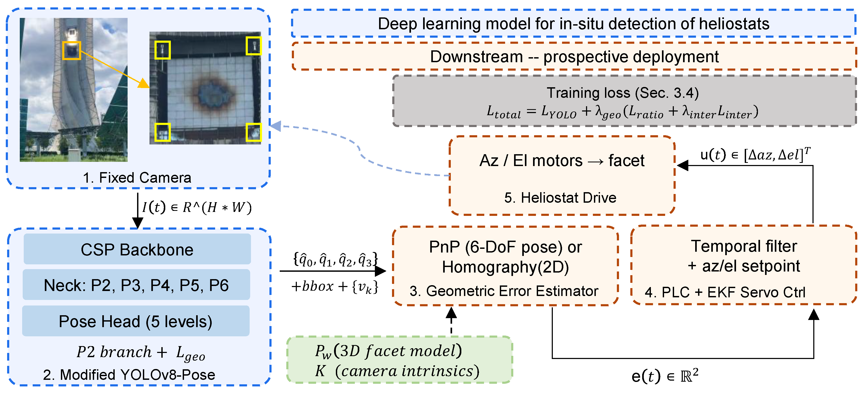
The proposed heliostat sensing system is a single-camera pipeline (Figure 1) that takes the input of images captured by cameras of various viewpoints and output the actual pose of heliostats in the world coordinate system to provide vision feedback for the tracking control of heliostats.

This pipeline frames the deep network not as a stand-alone classifier but as a component inserted into a control loop. Two design consequences follow. First, the output must be available at a frequency compatible with the servo control loop; for the prototype reported here, the end-to-end throughput is 25.14 FPS (Section 4), which is sufficient for the slow mechanical dynamics of a heliostat drive. Second, the per-frame output must be geometrically consistent: the four predicted corners must form a valid (non-self-intersecting, non-collapsed) quadrilateral that approximates the projected facet shape, otherwise the downstream controller would receive structurally invalid measurements and could execute large, abrupt commands.

3.2. Problem Formulation and Optical Challenges

The objective of this study is to perform high-speed and accurate localization of the four image-plane corners of a heliostat mirror from a monocular RGB image. Treating the four corners as the primary observable is deliberate: a rectangular facet is fully determined, up to a rigid-body pose with respect to the camera, by the projected positions of its four corners, and four 2D–3D correspondences are sufficient for a downstream PnP-style pose estimator [13,34]. Compared with detecting the full facet contour, four-corner detection is also markedly more robust under partial occlusion because losing one corner still leaves enough geometric information to flag the frame as degenerate and skip it.

Under a standard pinhole camera model, a 3D point ${\mathbf{P}}_w={[X_w,Y_w,Z_w,1]}^{\top }$ residing on the heliostat surface is mapped to the 2D image coordinate $\mathbf{p}={[x,y,1]}^{\top }$ via the perspective projection matrix:

$$z_c\mathbf{p}=\mathbf{K}[\mathbf{R}\mid \mathbf{t}]{\mathbf{P}}_w$$

(1)

where $\mathbf{K}$ is the camera intrinsic matrix, $[\mathbf{R}\mid \mathbf{t}]$ denotes the extrinsic pose parameters relative to the mirror, and $z_c$ is the depth of the 3D point in the camera frame (the homogeneous-coordinate scale factor). The symbol $z_c$ is reserved for this geometric depth and is distinct from the scalar loss weights ${\lambda }_{\mathrm{geo}}$ and ${\lambda }_{\mathrm{inter}}$ introduced later. Because $z_c$ varies continuously across the tilted mirror plane, affine properties—such as the parallelism between opposite edges of the rectangular mirror—are violated in the perspective image plane. Any structural regularization applied to the detection network therefore cannot rely on simplistic parallel-line assumptions, and must instead invoke projective invariants such as cross-ratios and line incidences [13].

Given an input image tensor $\mathbf{X}\in {\mathbb{R}}^{H\times W\times 3}$, the detection framework predicts, per visible facet, a set of four corner keypoints $\widehat{\mathbf{Q}}={\left\{{\widehat{\mathbf{q}}}_k\right\}}_{k=0}^3$, where ${\widehat{\mathbf{q}}}_k=({\widehat{x}}_k,{\widehat{y}}_k)$ denotes the predicted image coordinate of the k-th corner. The corresponding ground-truth set annotated by domain experts is denoted by $\mathbf{Q}={\left\{{\mathbf{q}}_k\right\}}_{k=0}^3$. We adopt a fixed corner ordering—top-left (TL), top-right (TR), bottom-left (BL), and bottom-right (BR)—during both annotation and prediction, so that diagonal correspondences (TL↔BR and TR↔BL) are well defined and can be used inside the geometric loss without combinatorial ambiguity.

The YOLOv8-Pose architecture is adopted as the baseline detector due to its highly efficient Cross Stage Partial (CSP) backbone, which is well-suited for industrial edge-computing deployments [30,35]. However, its default feature pyramid (relying heavily on P3 to P6 layers) entails excessive spatial downsampling, which over-smooths the high-frequency geometric discontinuities essential for precision metrology. Pixel-accurate corner localization in this regime is fundamentally limited by the receptive-field stride at the level from which the keypoint head reads its features; a pose head attached to P3–P6 only sees an effective stride of at least eight pixels relative to the input resolution, which is insufficient when the facet edge spans only a few tens of pixels in the captured image.

3.3. Resolution-Preserving Feature Fusion and Energy Analysis

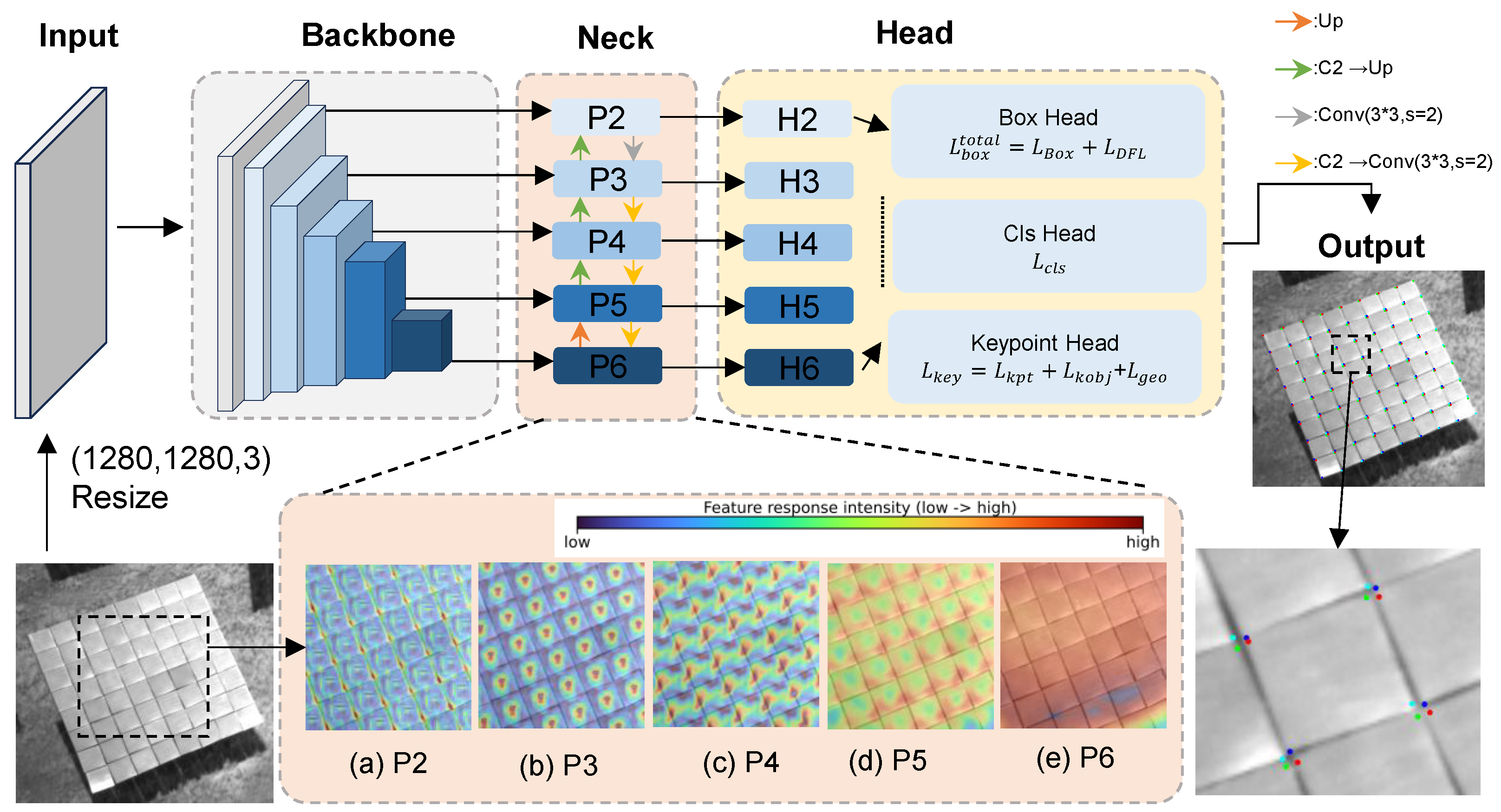
To address the critical attenuation of micro-structures at mirror boundaries, a high-resolution P2 feature level is integrated into the network’s neck (Figure 2). In the standard YOLOv8-Pose-P6 stack, the keypoint head receives features from levels P3 through P6, whose spatial strides relative to the input range from 8 to 64. We extend the multi-scale fusion path so that the keypoint head additionally reads a P2 feature with an effective stride of 4, which approximately doubles the spatial precision available at the head input without altering the backbone’s semantic depth or the pretrained weight initialization for the deeper levels [31,32]. To empirically validate this architectural intervention, we extract and quantify the feature response intensity across all pyramid levels. For a given feature tensor ${\mathbf{F}}^{\left(l\right)}\in {\mathbb{R}}^{C_l\times H_l\times W_l}$ at pyramid level l, the channel-wise activation is aggregated using root-mean-square (RMS) energy:

$$E^{\left(l\right)}(h,w)=\sqrt{{\displaystyle \frac{1}{C_l}}\sum _{c=1}^{C_l}{\left({\mathbf{F}}_c^{\left(l\right)}(h,w)\right)}^2}$$

(2)

Following a robust quantile normalization process to suppress background sensor noise, the resulting pseudo-color energy maps (Figure 2a–e) reveal a critical phenomenon: the P2 feature exhibits profound spatial convergence, tightly anchoring to the mirror’s physical boundaries. In contrast, deeper semantic levels (P5, P6) respond broadly to the global scene context, losing the localized precision needed for accurate few-pixel-level corner measurement. From the perspective of measurement, this is the expected behavior: deeper levels integrate large receptive fields that are useful for object presence but have already discarded the boundary location information by spatial pooling, whereas P2 retains short-range gradient cues that are co-located with the actual facet corners. Adding P2 into the head input therefore restores the high-frequency information that subsequent loss minimization can exploit; the deeper levels continue to contribute by gating the per-anchor visibility classification and confidence estimation.

3.4. Geometry Consistency Regularization Under Perspective Projection

The standard keypoint regression head in generic pose estimation architectures optimizes spatial coordinates by minimizing a visibility-masked distance metric:

$$L_{\mathrm{kpt}}={\displaystyle \frac{1}{N}}{\displaystyle \sum _{k=0}^3}{v}_k·\mathcal{D}({\widehat{\mathbf{q}}}_k,{\mathbf{q}}_k),$$

(3)

where $v_k\in \{0,1\}$ indicates keypoint visibility, and $\mathcal{D}$ typically represents the Object Keypoint Similarity (OKS) metric [36]. This point-wise, independent optimization carries no signal about the relative geometry of the four corners: it treats each corner in isolation and is indifferent to whether their joint configuration is consistent with a projected quadrilateral. Supplying this relative-geometry signal as an auxiliary supervision term is the role of $L_{\mathrm{geo}}$. In principle, such a term also guards against degenerate, self-intersecting configurations that a downstream geometric estimator could not interpret; in practice, these degeneracies do not arise on the present regular dataset (Section 4.1), and the measurable effect of $L_{\mathrm{geo}}$ is improved keypoint accuracy and robustness.

A naive remedy would be to penalize departures from a rigid rectangular shape, e.g., by enforcing parallel opposite edges or right angles. As discussed in Section 3, a rectangular facet projects to a non-rectangular quadrilateral under an off-axis pinhole projection, so such a penalty would push the network toward physically wrong predictions. The remedy must therefore be expressed in quantities that are invariant under the perspective projection. We choose two such invariants and combine them.

Without violating perspective geometry, the geometry-consistency loss ($L_{\mathrm{geo}}$) is therefore formulated from perspective-compatible geometric quantities, i.e., quantities whose target values are read from the ground-truth projection rather than from a planar-rectangle prior. The first component evaluates the scale-invariant geometric edge-ratio ($L_{\mathrm{ratio}}$):

$$L_{\mathrm{ratio}}=\left|log{\displaystyle \frac{d({\widehat{\mathbf{q}}}_0,{\widehat{\mathbf{q}}}_1)}{d({\widehat{\mathbf{q}}}_2,{\widehat{\mathbf{q}}}_3)}}-log{\displaystyle \frac{d({\mathbf{q}}_0,{\mathbf{q}}_1)}{d({\mathbf{q}}_2,{\mathbf{q}}_3)}}\right|+\left|log{\displaystyle \frac{d({\widehat{\mathbf{q}}}_0,{\widehat{\mathbf{q}}}_2)}{d({\widehat{\mathbf{q}}}_1,{\widehat{\mathbf{q}}}_3)}}-log{\displaystyle \frac{d({\mathbf{q}}_0,{\mathbf{q}}_2)}{d({\mathbf{q}}_1,{\mathbf{q}}_3)}}\right|$$

(4)

where $d(\mathbf{a},\mathbf{b})={\parallel \mathbf{b}-\mathbf{a}\parallel }_2$ denotes the Euclidean distance. The use of the logarithm has two pragmatic effects. First, it converts a multiplicative ratio mismatch into an additive scale-symmetric penalty, so that a 10% error on a small edge contributes the same loss magnitude as a 10% error on a large edge. Second, it removes the numerical asymmetry that a raw ratio would introduce when an edge is short. To prevent log singularities for very small edges, the implementation clamps both numerator and denominator to a small positive lower bound before taking the logarithm.

The second component enforces diagonal-intersection consistency ($L_{\mathrm{inter}}$). Let $L_1=\parallel {\mathbf{q}}_3-{\mathbf{q}}_0\parallel$ and $L_2=\parallel {\mathbf{q}}_2-{\mathbf{q}}_1\parallel$ denote the two diagonal lengths, and let

$${\widehat{\mathbf{d}}}_1={\displaystyle \frac{{\mathbf{q}}_3-{\mathbf{q}}_0}{L_1}},{\widehat{\mathbf{d}}}_2={\displaystyle \frac{{\mathbf{q}}_2-{\mathbf{q}}_1}{L_2}}$$

(5)

denote the corresponding unit-norm direction vectors ($\parallel {\widehat{\mathbf{d}}}_1\parallel =\parallel {\widehat{\mathbf{d}}}_2\parallel =1$). The two ground-truth diagonals are then parameterized by arc length as ${\ell }_1\left(s\right)={\mathbf{q}}_0+s{\widehat{\mathbf{d}}}_1$ and ${\ell }_2\left(t\right)={\mathbf{q}}_1+t{\widehat{\mathbf{d}}}_2$, where $s\in [0,L_1]$ and $t\in [0,L_2]$ are measured directly in image-plane pixels. Their intersection $\mathbf{I}$ must satisfy

$${\mathbf{q}}_0+s{\widehat{\mathbf{d}}}_1={\mathbf{q}}_1+t{\widehat{\mathbf{d}}}_2.$$

(6)

Taking the 2D cross product of both sides with ${\widehat{\mathbf{d}}}_2$ eliminates t and yields the closed-form solution

$$s={\displaystyle \frac{det\left({\mathbf{q}}_1-{\mathbf{q}}_0,{\widehat{\mathbf{d}}}_2\right)}{det\left({\widehat{\mathbf{d}}}_1,{\widehat{\mathbf{d}}}_2\right)+\epsilon }}={\displaystyle \frac{det\left({\mathbf{q}}_1-{\mathbf{q}}_0,{\widehat{\mathbf{d}}}_2\right)}{sin\theta +\epsilon }},$$

(7)

where $\theta$ is the angle between ${\widehat{\mathbf{d}}}_1$ and ${\widehat{\mathbf{d}}}_2$, and $\epsilon$ is a small positive constant that prevents division by zero when the two diagonals become nearly collinear ($\theta \to 0$). Because ${\widehat{\mathbf{d}}}_1$ and ${\widehat{\mathbf{d}}}_2$ are unit-norm, $det({\widehat{\mathbf{d}}}_1,{\widehat{\mathbf{d}}}_2)$ is exactly $sin\theta$, so $\epsilon$ acquires the clear physical meaning of a lower bound on the admissible angular separation of the two diagonals rather than the role of a purely numerical safeguard.

The ground-truth intersection follows from Equation (7) in one line as $\mathbf{I}={\mathbf{q}}_0+s{\widehat{\mathbf{d}}}_1$. The predicted intersection $\widehat{\mathbf{I}}$ is computed by the same closed form applied to the predicted corner set $\widehat{\mathbf{Q}}$—i.e., by substituting ${\widehat{\mathbf{q}}}_k$ for ${\mathbf{q}}_k$ throughout Equations (5)–(7)—and the Euclidean distance between the two intersection points serves as the structural penalty

$$L_{\mathrm{inter}}=\parallel \widehat{\mathbf{I}}-\mathbf{I}{\parallel }_2.$$

(8)

The intersection points are expressed in normalized image coordinates (pixel coordinates divided by the input image size) before this distance is evaluated, so $L_{\mathrm{inter}}$ is dimensionless and is directly comparable in magnitude with $L_{\mathrm{ratio}}$.

Geometrically, $L_{\mathrm{inter}}$ penalizes configurations in which the two predicted diagonals fail to meet at the same projected point as the ground-truth diagonals. Because the cross-ratio along each diagonal is preserved by the perspective projection [13], requiring the two predicted diagonals to intersect at the correct projected point is equivalent to requiring the projected facet to have the correct internal cross-ratio structure—without imposing parallelism, right angles, or rectangularity in the image plane. $L_{\mathrm{inter}}$ is therefore a perspective-invariant geometric regularizer, complementary to the image-plane edge-length-ratio regularizer $L_{\mathrm{ratio}}$ of Equation (4), which constrains scale consistency along the facet sides rather than the projective incidence of the diagonals.

The complete training objective combines this geometric regularizer with the standard YOLO bounding-box, classification and keypoint terms:

$$L_{\mathrm{total}}=L_{\mathrm{YOLO}}+{\lambda }_{\mathrm{geo}}\left(L_{\mathrm{ratio}}+{\lambda }_{\mathrm{inter}}{L}_{\mathrm{inter}}\right).$$

(9)

In our reference implementation, the geometric weight ${\lambda }_{\mathrm{geo}}$ is held at a small value so that $L_{\mathrm{geo}}=L_{\mathrm{ratio}}+{\lambda }_{\mathrm{inter}}{L}_{\mathrm{inter}}$ behaves as an auxiliary regularizer rather than as a primary objective: it injects a relative-geometry signal that shapes the search space while leaving the bulk of the gradient to the standard keypoint and bounding-box terms. The loss is clipped to a finite range so that the gradient remains bounded when degenerate, near-parallel-diagonal configurations briefly appear early in training—that is, when $sin\theta \to 0$ in Equation (7) and the closed-form s would otherwise dominate the optimization step.

3.5. Dataset and Annotation

The proposed framework was evaluated on an industrial heliostat image dataset. The dataset comprises 300 high-resolution images of operating heliostats captured at various times of day. The four corner points of each facet of the heliostat in the image are labeled in a fixed TL/TR/BL/BR order, together with a visibility flag, so that the geometric loss in Section 3 can be computed only over fully visible facets. The dataset is treated as a self-contained engineering benchmark rather than a public competition task. It serves as a testbed for evaluating deep learning methods for the detection and control of heliostats in a CSP plant [11].

Each image contains a single heliostat composed of an $8\times 8$ grid of sub-mirror facets, yielding $64\times 4=256$ corner annotations per fully visible image. Corners that fall inside saturated (over-exposed) or shadowed (under-exposed) regions are intentionally not annotated and are excluded from the loss by the per-keypoint visibility flag $v_k$ (see Equation (3)); this convention propagates the optical-degradation statistics of the deployment scene into the supervision signal rather than into the labelling protocol. The 300 images are split at the image level into train, validation and test partitions in an 8:1:1 ratio (240/30/30 images), corresponding to up to 61,440/7680/7680 annotated corners under the fully visible upper bound.

3.6. Implementation Details

The model was trained on an NVIDIA RTX 4090D GPU using the AdamW optimizer [37] for 300 epochs, with input tensors resized to $1280\times 1280$ to fully leverage the high-resolution P2 capabilities. Mixed-precision (AMP) computation was enabled to reduce GPU memory pressure, and the keypoint-loss gain was raised relative to the default value to align the optimization budget with the precision-driven objective of this work. Geometric data augmentation was deliberately conservative (small rotation, small translation, small scale, no synthetic perspective warp) so that the model is exposed to operationally realistic facet shapes rather than to aggressively warped quadrilaterals; mosaic and a small mixup factor were retained so that anchor-based pose detection still benefits from multi-instance composition during training. The optimizer used an initial learning rate of $5\times {10}^{-4}$ with a cosine schedule, and the geometry weight was set to ${\lambda }_{\mathrm{geo}}=0.05$; all other settings followed the YOLOv8-Pose defaults.

3.7. Evaluation Metrics

For evaluation, we use four metrics. mAP@0.5 reports the average precision under a relatively loose IoU threshold and quantifies whether the facet is found at all. mAP@0.5:0.95 averages precision over a sweep of stricter IoU thresholds and is therefore the most sensitive to localization accuracy of the bounding box that surrounds the four keypoints. AR@0.5 reports the average recall under the loose IoU threshold and complements precision by quantifying how often a present facet is missed. End-point error (EPE) is the mean Euclidean distance between predicted and ground-truth keypoint coordinates over matched detections. End-to-end frames per second (FPS) is reported as the wall-clock throughput including pre-processing, inference, and post-processing.

4. Results and Discussion

4.1. Main Ablation and Topology Check

Table 1. Ablation on the test set. The high-resolution P2 branch is the dominant source of the keypoint-accuracy gain; adding the geometry loss $L_{\mathrm{geo}}$ (Ours) yields the lowest end-point error at essentially unchanged detection precision. The proposed configuration and the best value in each column are shown in bold. Upward and downward arrows indicate that higher and lower values are better, respectively.

Model Configuration	mAP@0.5 ↑	mAP@0.5:0.95 ↑	EPE (px) ↓
Baseline YOLOv8-Pose	0.9903	0.9671	2.22
Only_Geo	0.9883	0.9656	2.39
Only_P2	0.9936	0.9847	1.24
Ours (P2_Geo)	0.9927	0.9823	1.22

isolates the two proposed components. P2 reduced EPE from 2.22 to 1.24 px while increasing mAP@0.5:0.95 from 0.9671 to 0.9847, making it the main source of the accuracy gain. Adding $L_{\mathrm{geo}}$ to P2 further reduced EPE to 1.22 px, whereas applying the loss without P2 increased EPE to 2.39 px. The following analyses therefore evaluate $L_{\mathrm{geo}}$ as an auxiliary regularizer rather than an independent source of spatial resolution.

We tested the topological-stability hypothesis using self-intersection, concavity, degeneracy, and invalid-quadrilateral rates. All configurations achieved 0.00% on these metrics over 655–663 fully visible matched facets. The normalized diagonal-intersection deviations were 0.0025, 0.0031, 0.0015, and 0.0016 for Baseline, Only_Geo, Only_P2, and Ours, respectively. These results do not support a topology-improvement claim; instead, the experiments below support $L_{\mathrm{geo}}$ as a regularizer under limited data and degraded inputs.

4.2. Weight Sensitivity and Run-to-Run Variability

We varied ${\lambda }_{\mathrm{geo}}\in \{0,0.01,0.02,0.05,0.1,0.2,0.5\}$ on the P2 model while fixing all other settings and using a shared seed. Setting ${\lambda }_{\mathrm{geo}}=0$ disabled $L_{\mathrm{geo}}$. This experiment tested whether the regularizer remained effective over a stable range rather than at a narrowly tuned weight.

Table 2. Sensitivity to the geometric weight ${\lambda }_{\mathrm{geo}}$ (P2 model, single shared seed; ${\lambda }_{\mathrm{geo}}=0$ disables $L_{\mathrm{geo}}$). The invalid-quadrilateral rate is $0.00\%$ at every weight and is omitted. The selected weight is shown in bold. Upward and downward arrows indicate that higher and lower values are better, respectively.

${\mathit{\lambda }}_{\mathbf{geo}}$	mAP@0.5:0.95 ↑	EPE (px) ↓
0.00 (no $L_{\mathrm{geo}}$)	0.9819	1.379
0.01	0.9856	1.222
0.02	0.9817	1.224
0.05 (used)	0.9841	1.231
0.10	0.9827	1.232
0.20	0.9843	1.266
0.50	0.9855	1.277

reports the sensitivity results across the tested weights.

For ${\lambda }_{\mathrm{geo}}\in [0.01,0.10]$, EPE ranged from 1.221 to 1.232 px, compared with 1.379 px without $L_{\mathrm{geo}}$, while mAP@0.5:0.95 ranged from 0.982 to 0.986. The 0.011 px spread was smaller than the 0.051 px run-to-run standard deviation reported below. The tested weights within this plateau were therefore not meaningfully distinguishable, and we selected ${\lambda }_{\mathrm{geo}}=0.05$ as a central value. At weights of 0.2 and 0.5, EPE increased to 1.266 and 1.277 px, respectively, indicating interference with keypoint regression.

To assess run-to-run variability, we retrained the baseline and the proposed model with five random seeds (0–4) and evaluated all runs on the fixed test set.

Table 3. Run-to-run variability over five random seeds (mean ± std; 95% CI in brackets). The invalid-quadrilateral rate is $0.00\%$ for every seed of both configurations. The proposed model and its values are shown in bold. Upward and downward arrows indicate that higher and lower values are better, respectively.

Model Configuration	EPE (px) ↓	mAP@0.5:0.95 ↑
Baseline YOLOv8-Pose	$2.071\pm 0.193$ [1.831, 2.311]	$0.9720\pm 0.0037$ [0.9675, 0.9766]
Ours (P2_Geo)	1.282 ± 0.051 [1.219, 1.345]	0.9839 ± 0.0006 [0.9831, 0.9847]

reports the mean, standard deviation, and 95% confidence interval based on Student’s t distribution ($\mathrm{dof}=4$).

Across five seeds, the proposed model reduces mean EPE by 0.79 px (38%) relative to the baseline. The 95% confidence intervals are disjoint ([1.831, 2.311] versus [1.219, 1.345]), and the difference is significant under both a two-sided Welch t-test ($p=5.0\times {10}^{-4}$) and a Mann–Whitney U test ($p=7.9\times {10}^{-3}$). Its EPE and mAP standard deviations were lower by factors of 3.8 and 6.0, respectively, indicating lower sensitivity to random seeds. The 1.22 px result in Table 1 lies within the proposed model’s confidence interval.

4.3. Robustness Under the Condition of Limit Data and Image Degradation

We first evaluated $L_{\mathrm{geo}}$ at three training fractions. Its EPE advantage over Only_P2 increased from 0.147 px at 100% of the training data to 0.366 px at 50% and 1.361 px at 25% (

Table 4. Data-efficiency ablation of the P2 model without and with $L_{\mathrm{geo}}$ at three training fractions. Positive $\Delta$EPE values indicate lower error for the proposed model. The lowest EPE in each row is shown in bold. Downward arrows indicate that lower values are better.

Training Data	Only_P2 EPE ↓	Ours EPE ↓	$\mathbf{\Delta }$EPE	mAP@0.5:0.95 (P2/Ours)
25%	3.725	2.364	$+1.361$	0.885/0.930
50%	1.960	1.593	$+0.366$	0.982/0.983
100%	1.379	1.231	$+0.147$	0.982/0.984

). This experiment examined whether geometric supervision became more useful when labeled training data were limited.

The benefit of $L_{\mathrm{geo}}$ increased as the training fraction decreased. At 25%, it reduced EPE by 37% (3.725 to 2.364 px) and increased mAP@0.5:0.95 from 0.885 to 0.930. This trend supports the interpretation of $L_{\mathrm{geo}}$ as a regularizer that is particularly useful under limited supervision.

We next degraded the test images without retraining by adding Gaussian noise, applying Gaussian blur, and reducing resolution. Invalid-quadrilateral rates remained approximately zero across the tested conditions, apart from one 0.156% case. Thus, degradation mainly caused missed detections and localization error rather than malformed quadrilaterals. Under resolution loss, Ours retained lower EPE than Only_P2, including 1.43 versus 2.17 px at $0.50\times$ resolution and 1.84 versus 3.22 px at $0.35\times$ resolution (

Table 5. EPE under progressive resolution loss. Ours denotes the P2 model trained with $L_{\mathrm{geo}}$. The lowest EPE in each row is shown in bold.

Downscale Factor	Baseline	Only_P2	Ours
$1.00$	2.22	1.24	1.22
$0.75$	2.30	1.37	1.32
$0.50$	2.34	2.17	1.43
$0.35$	2.46	3.22	1.84
$0.25$	2.75	2.47	2.32

). At a noise standard deviation of $20/255$, Ours retained 8.9% of detections, compared with 3.3% for Only_P2 and none for the baseline.

Together, the limited-data and degradation experiments show that $L_{\mathrm{geo}}$ provides its clearest benefit when the available visual evidence is reduced.

4.4. Comparison with a Generic Pose Estimator and Qualitative Analysis

We evaluated MMPose under its default top-down configuration on the same heliostat dataset [38]. It achieved an mAP@0.5 of 0.3267 and an AR@0.5 of 0.3207, compared with an mAP@0.5 of 0.9927 for the proposed model (Table 1). Its EPE of 2.0139 px was computed only for detected facets and is therefore not directly comparable with the larger set of matched facets produced by our detector. This result indicates that the tested generic human-pose pipeline does not transfer directly to texture-poor, specular heliostat facets. OpenPose and SimpleBaseline provide broader human-pose context for this comparison [25,26].

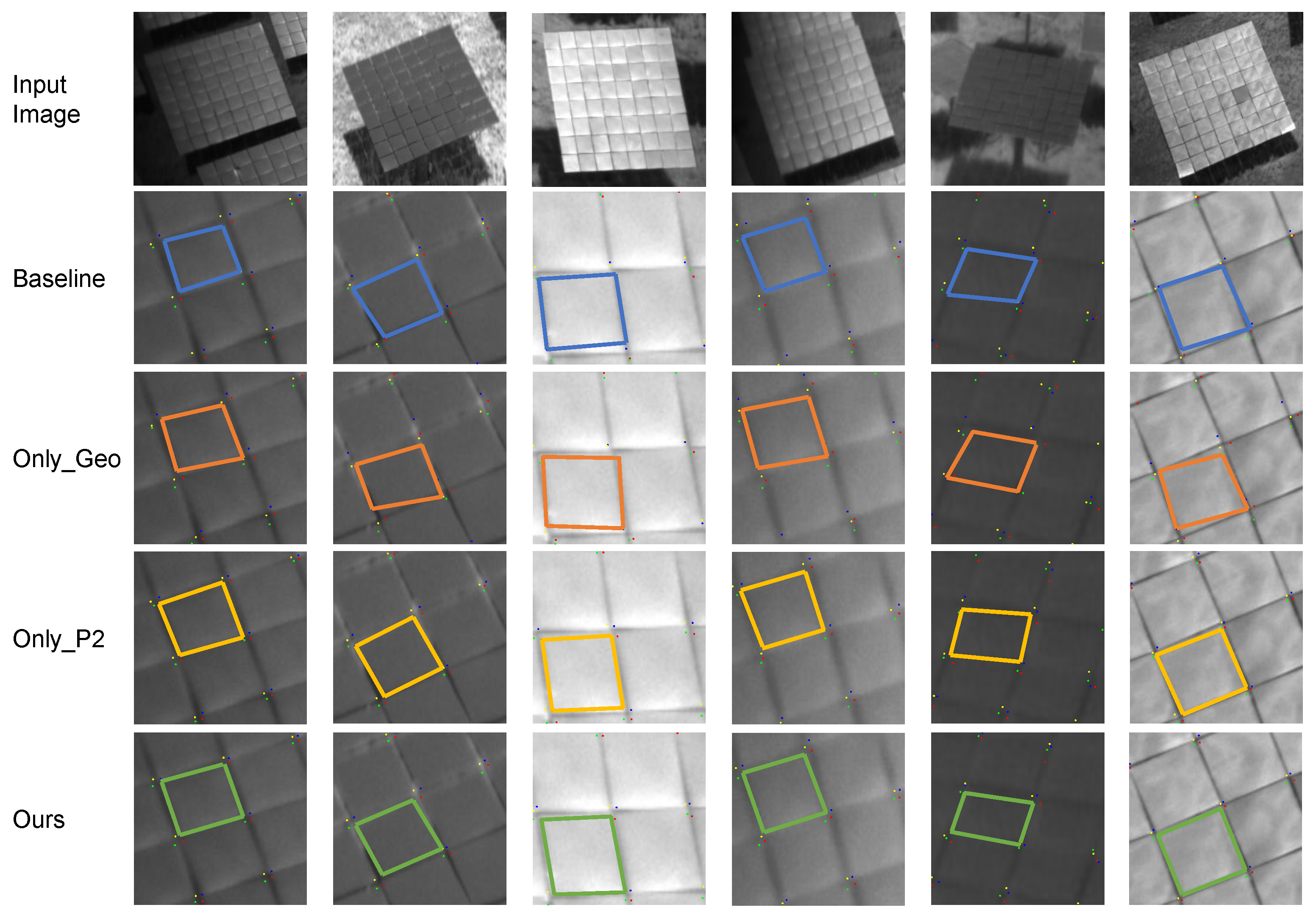
Figure 3 compares corner localization across the four ablation configurations under challenging illumination.

The baseline corners are less tightly aligned with the facet boundaries, particularly in saturated or blurred regions, whereas the P2-based models show more accurate localization. These differences concern localization rather than topology because no configuration produces self-intersecting or degenerate quadrilaterals on the test set (Section 4.1). The visual comparison therefore supports the quantitative finding that P2 provides most of the spatial improvement. The contribution of $L_{\mathrm{geo}}$ is established more clearly by the sensitivity and robustness results in Table 2 and Table 5.

4.5. Runtime and Deployment Considerations

This subsection evaluates the localization accuracy, runtime, computational cost, and calibration requirements relevant to prospective field deployment.

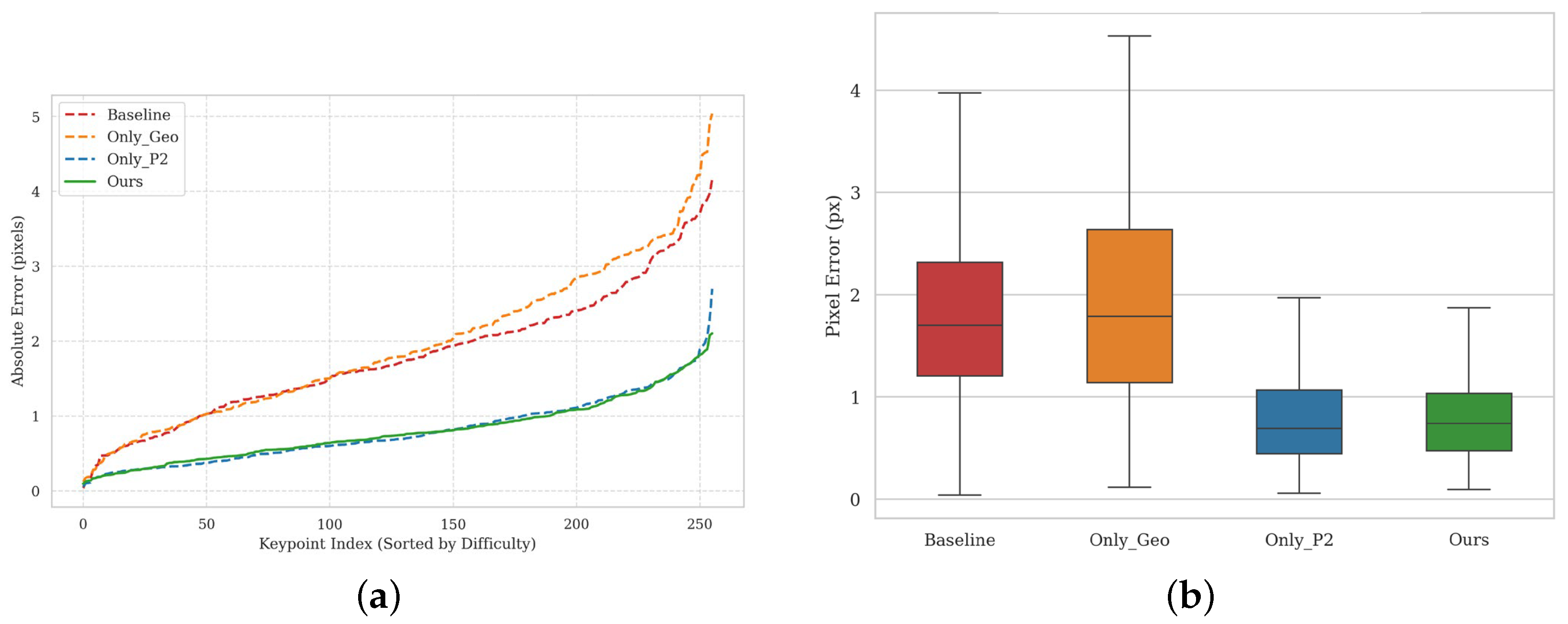
The proposed model achieves a mean EPE of 1.22 px under outdoor glare and local saturation without iterative sub-pixel refinement. Figure 4 therefore examines the full error distribution rather than only its mean.

Enabling $L_{\mathrm{geo}}$ reduces the 95th-percentile error from 2.80 to 2.57 px (Figure 4). A smaller upper tail may reduce large frame-to-frame corrections in a downstream controller, but this effect requires closed-loop validation.

Table 6. Measured runtime of the proposed framework on the desktop evaluation platform.

Performance Metric	Measured Value
End-to-end FPS (wall-clock) ↑	25.14
Inference-only FPS ↑	27.51
Pre-process time (ms) ↓	1.996
Inference time (ms) ↓	36.349
Post-process time (ms) ↓	0.784

reports the measured runtime of the complete evaluation pipeline on the desktop platform. The system processes 25.14 frames per second end to end, including preprocessing, inference, and post-processing.

The measured throughput exceeds the sampling frequency implied by the solar tracking rate of approximately ${15}^{\circ }$ per hour. However, complete closed-loop latency also includes image acquisition, communication, filtering, and actuator response.

The P2 accuracy gain increases computational cost. At $1280\times 1280$, the proposed model contains 94.77 M parameters and requires 1290 GFLOPs, compared with 4.89 M parameters and 33.7 GFLOPs for the P6-only baseline.

Table 7. Model-only inference latency for the proposed model at $1280\times 1280$ and batch size 1. The RTX 4090D result is measured; Jetson results are throughput-scaled FP16 estimates.

Device (Precision)	Inference (ms) ↓	Inference FPS ↑
RTX 4090D (FP16, measured)	23.2	43.1
Jetson AGX Orin 64GB (FP16, estimate)	∼90	∼11.1
Jetson Orin NX 16GB (FP16, estimate)	∼153	∼6.5
Jetson Orin Nano 8GB (FP16, estimate)	∼383	∼2.6

reports the measured desktop result and throughput-scaled Jetson estimates. The Jetson values are feasibility estimates rather than device measurements.

The estimates in Table 7 indicate that edge deployment is computationally plausible, but direct measurements are required on the target hardware. Quantization, pruning, or distillation may reduce memory and computational cost, although their effects on localization accuracy must be evaluated.

Field deployment also requires stable camera geometry and controlled image acquisition. A rigid mount and periodic calibration are needed to limit intrinsic and extrinsic errors [12,13]. Exposure control or high-dynamic-range acquisition is important because saturation removes the local gradients required for corner localization [18,19].

The detected corners can support planar pose estimation with a calibrated camera and a known target model [34]. Short-window temporal filtering may reduce frame-level jitter [39], while edge inference may avoid network-induced delay [35]. Integration with calibration, filtering, and actuator control remains future work.

4.6. Pixel-to-Pointing Error and Influence of Camera Calibration Error

We use an open-loop error-propagation analysis to examine how image-space corner error affects heliostat position and orientation estimates. The analysis characterizes a prospective downstream pose stage and does not constitute closed-loop validation.

Let ${\sigma }_{\mathrm{px}}$ denote the image-space corner-noise level, f the focal length in pixels, Z the camera–target range, A the physical aperture of the keypoint constellation, and n the number of corners. The ground sampling distance is $g=Z/f$. The transverse position error of the constellation centroid is approximated by

$${\sigma }_{t\perp }\approx {\displaystyle \frac{Z}{f}}{\displaystyle \frac{{\sigma }_{\mathrm{px}}}{\sqrt{n}}}=g{\displaystyle \frac{{\sigma }_{\mathrm{px}}}{\sqrt{n}}}.$$

(10)

Range and out-of-plane orientation are less well conditioned because they are observed through perspective foreshortening. For a tilt $\alpha$ about an in-plane axis, a conservative single-cue sensitivity estimate based on the projected edge-length difference is

$${\sigma }_{\alpha }\approx {\displaystyle \frac{2{\sigma }_{\mathrm{px}}{Z}^2}{f{A}^{2}cos\alpha }},$$

(11)

A least-squares fit over all n corners reduces this error by approximately $\sqrt{n}$. By the law of reflection, the reflected-beam error is twice the surface-normal error, ${\sigma }_{\mathrm{beam}}\approx 2{\sigma }_{\alpha }$, and the receiver-spot displacement is ${\Delta }_{\mathrm{spot}}\approx 2{\sigma }_{\alpha }D$ at slant range D. Equations (10) and (11) show the expected dependence on image error, range, focal length, and target aperture.

The Monte Carlo simulation uses the measured camera intrinsics ($f_x\approx 3513$ px and $f_y\approx 3510$ px), a 10.36 m square target, planar IPPE, and 2000 samples per condition. The zero-noise case yields 0.000 mrad. Within the tested grid, the estimated normal error follows an empirical relation of approximately 0.142 mrad per pixel of EPE per meter of range.

Table 8. Simulated surface-normal and reflected-beam errors versus camera–target range using the measured intrinsics, a 10.36 m square target, and planar IPPE.

Z (m)	Ours, Normal (mrad)	Baseline, Normal (mrad)	Ours, Beam (mrad)
20	3.5	6.3	6.9
40	6.9	12.6	13.9
60	10.4	18.9	20.8
80	13.9	25.2	27.7
100	17.3	31.5	34.6

reports the corresponding normal and reflected-beam errors. At 40 m, the 1.22 px result gives an estimated normal error of 6.9 mrad, compared with 12.6 mrad for the 2.22 px baseline.

The simulation assumes that corner error is the dominant uncertainty and that the target is observed from a well-conditioned, non-frontoparallel viewpoint. Near-frontoparallel views introduce a two-fold tilt ambiguity. The results therefore quantify an open-loop error-propagation trend; temporal ambiguity resolution and physical closed-loop validation remain future work.

Detector error is only one component of the pointing-error budget because intrinsic and extrinsic calibration errors also contribute. A first-order variance decomposition is

$${\sigma }_{\alpha ,\mathrm{total}}^2\approx \underset{\mathrm{detector}}{\underbrace{{\sigma }_{\alpha ,\det }^2}}+\underset{\mathrm{extrinsic}}{\underbrace{\delta R^2}}+\underset{\mathrm{intrinsic}}{\underbrace{\kappa {\left({\displaystyle \frac{\delta f}{f}}\right)}^2+{\left({\displaystyle \frac{\delta c}{a_{\mathrm{px}}}}\right)}^2}},$$

(12)

Here, ${\sigma }_{\alpha ,\det }$ is the detector-induced normal error, $\delta R$ is the camera-orientation error, $\delta f/f$ is the relative focal-length error, $\delta c$ is the principal-point error, and $\kappa =\mathcal{O}\left(1\right)$. The perturbation study at $Z=40$ m follows the ordering in Equation (12): focal-length and camera-orientation errors have the largest effects, whereas the tested principal-point and camera-position perturbations have little effect on the recovered angle (

Table 9. Monte Carlo sensitivity of the recovered surface-normal error to calibration perturbations at $Z=40$ m. The detector-only reference uses a 1.89 px noise level; the ranking of calibration effects is the focus of this analysis.

Perturbed Quantity	Magnitude	Normal Error (mrad)
None (detector only)	—	10.9
Focal length $\delta f/f$	$1\%$	34.8
Focal length $\delta f/f$	$5\%$	137.4
Principal point $\delta c$	10 px	11.3
Camera orientation $\delta R$	$1^{\circ }$	17.1
Camera orientation $\delta R$	$2^{\circ }$	29.3
Camera position $\delta t$	2 m	10.7

). These results imply that rigid mounting and periodic calibration of cameras are very important.

5. Conclusions

A high-speed, geometry-aware visual measurement framework for in situ detection of heliostats in concentrated solar power plants is proposed in the paper. By integrating YOLOv8-Pose architecture with a high-resolution P2 branch and adapting a specific perspective-compatible geometry-consistency loss function, the framework recovers fine-grain boundary information and achieved a higher accuracy of geometric keypoints detection within an outdoor environment, with the mean EPE around 1.22 px with the real-world dataset. The deep learning-based framework achieved an end-to-end processing speed of 25.14 FPS. Although the experiments were carried out at a small-scale CSP station, the methodology is applicable to large-scale commercial CSP plants.

The focus of this paper is on in situ detection of 2D image keypoints rather than pose estimation algorithms. The deep learning framework outputs the image coordinates of the keypoints of the mirror facets. The on-line estimation of heliostat tracking pose can be done using these keypoints and another module that combine optimization and EPnP algorithms [14].

It must be pointed out that the reported throughput (25.14 FPS) is based on the specified hardware. In-field processing speed relies on the computation speed and memory size of the deployed hardware. In our opinion, the backbone network may be further compressed via channel pruning, knowledge-distillation, etc., to accelerate the processing speed on the target platform [35]. Such compression is feasible because the geometric constraints are imposed at the training stage rather than the inference stage.

References

1. Islam, M.T.; Huda, N.; Abdullah, A.B.; Saidur, R. A Comprehensive Review of State-of-the-Art Concentrating Solar Power (CSP) Technologies: Current Status and Research Trends. Renew. Sustain. Energy Rev. 2018, 91, 987–1018. [Google Scholar] [CrossRef]
2. Ho, C.K. Advances in Central Receivers for Concentrating Solar Applications. Sol. Energy 2017, 152, 38–56. [Google Scholar] [CrossRef]
3. Noone, C.J.; Torrilhon, M.; Mitsos, A. Heliostat Field Optimization: A New Computationally Efficient Model and Biomimetic Layout. Sol. Energy 2012, 86, 792–803. [Google Scholar] [CrossRef]
4. Maiga, M.; N’Tsoukpoe, K.E.; Gomna, A.; Fiagbe, Y.A.K. Sources of Solar Tracking Errors and Correction Strategies for Heliostats. Renew. Sustain. Energy Rev. 2024, 203, 114770. [Google Scholar] [CrossRef]
5. Berenguel, M.; Rubio, F.R.; Valverde, A.; Lara, P.J.; Arahal, M.R.; Camacho, E.F.; López, M. An Artificial Vision-Based Control System for Automatic Heliostat Positioning Offset Correction in a Central Receiver Solar Power Plant. Sol. Energy 2004, 76, 563–575. [Google Scholar] [CrossRef]
6. Phipps, G.S. Heliostat Beam Characterization System–Calibration Technique. In Proceedings of the ISA/79 Conference, Chicago, IL, USA, October 1979; Report SAND-79-1532C. Available online: https://www.osti.gov/biblio/6079363 (accessed on 8 July 2026).
7. Röger, M.; Herrmann, P.; Ulmer, S.; Ebert, M.; Prahl, C.; Göhring, F. Techniques to Measure Solar Flux Density Distribution on Large-Scale Receivers. J. Sol. Energy Eng. 2014, 136, 031013. [Google Scholar] [CrossRef]
8. Mehos, M.; Price, H.; Cable, R.; Kearney, D.; Kelly, B.; Kolb, G.; Morse, F. Concentrating Solar Power Best Practices Study; Technical Report NREL/TP-5500-75763; National Renewable Energy Laboratory: Golden, CO, USA, 2020. [Google Scholar] [CrossRef] [PubMed]
9. Prahl, C.; Stanicki, B.; Hilgert, C.; Ulmer, S.; Röger, M. Airborne Shape Measurement of Parabolic Trough Collector Fields. Sol. Energy 2013, 91, 68–78. [Google Scholar] [CrossRef]
10. Chaumette, F.; Hutchinson, S. Visual Servo Control. I. Basic Approaches. IEEE Robot. Autom. Mag. 2006, 13, 82–90. [Google Scholar] [CrossRef]
11. Steger, C.; Ulrich, M.; Wiedemann, C. Machine Vision Algorithms and Applications, 2nd ed.; Wiley-VCH: Weinheim, Germany, 2018. [Google Scholar]
12. Zhang, Z. A Flexible New Technique for Camera Calibration. IEEE Trans. Pattern Anal. Mach. Intell. 2000, 22, 1330–1334. [Google Scholar] [CrossRef]
13. Hartley, R.; Zisserman, A. Multiple View Geometry in Computer Vision, 2nd ed.; Cambridge University Press: Cambridge, UK, 2004. [Google Scholar] [CrossRef]
14. Xu, F.; Li, C.; Sun, F. On-Line Measurement of Tracking Poses of Heliostats in Concentrated Solar Power Plants. Sensors 2024, 24, 6373. [Google Scholar] [CrossRef] [PubMed]
15. Pargmann, M.; Quinto, D.M.; Schwarzbözl, P.; Pitz-Paal, R. Automatic Heliostat Learning for In Situ Concentrating Solar Power Plant Metrology with Differentiable Ray Tracing. Nat. Commun. 2024, 15, 6997. [Google Scholar] [CrossRef] [PubMed]
16. Lewen, J.; Pargmann, M.; Cherti, M.; Jitsev, J.; Pitz-Paal, R.; Maldonado Quinto, D. Inverse Deep Learning Raytracing for Heliostat Surface Prediction. Sol. Energy 2025, 289, 113312. [Google Scholar] [CrossRef]
17. Balakrishnan, P. Artificial Intelligence in Heliostat Control and Optimization for CSP Plants: A Critical Review. Renew. Sustain. Energy Rev. 2026, 229, 116637. [Google Scholar] [CrossRef]
18. Nayar, S.K.; Fang, X.S.; Boult, T. Separation of Reflection Components Using Color and Polarization. Int. J. Comput. Vis. 1997, 21, 163–186. [Google Scholar] [CrossRef]
19. Debevec, P.E.; Malik, J. Recovering High Dynamic Range Radiance Maps from Photographs. In Proceedings of the SIGGRAPH 1997; ACM Press: New York, NY, USA, 1997; pp. 369–378. [Google Scholar] [CrossRef]
20. Qiu, J.M.; Jiang, P.S.; Zhu, Y.; Yin, Z.X.; Cheng, M.M.; Mu, T.J. Looking Through the Glass: Neural Surface Reconstruction Against High Specular Reflections. In Proceedings of the IEEE/CVF Conference on Computer Vision and Pattern Recognition (CVPR); IEEE: Piscataway, NJ, USA, 2023; pp. 20823–20833. [Google Scholar] [CrossRef]
21. Han, Y.; Guo, H.; Fukai, K.; Santo, H.; Shi, B.; Okura, F.; Ma, Z.; Jia, Y. NeRSP: Neural 3D Reconstruction for Reflective Objects with Sparse Polarized Images. In Proceedings of the IEEE/CVF Conference on Computer Vision and Pattern Recognition (CVPR); IEEE: Piscataway, NJ, USA, 2024; pp. 11821–11830. [Google Scholar] [CrossRef]
22. Tang, J.; Fei, F.; Li, Z.; Tang, X.; Liu, S.; Chen, Y.; Huang, B.; Chen, Z.; Wu, X.; Shi, B. SpecTRe-GS: Modeling Highly Specular Surfaces with Reflected Nearby Objects by Tracing Rays in 3D Gaussian Splatting. In Proceedings of the IEEE/CVF Conference on Computer Vision and Pattern Recognition (CVPR); IEEE: Piscataway, NJ, USA, 2025; pp. 16133–16142. [Google Scholar] [CrossRef]
23. Newell, A.; Yang, K.; Deng, J. Stacked Hourglass Networks for Human Pose Estimation. In Proceedings of the Computer Vision—ECCV 2016; Lecture Notes in Computer Science; Springer: Cham, Switzerland, 2016; Volume 9912, pp. 483–499. [Google Scholar] [CrossRef]
24. Toshev, A.; Szegedy, C. DeepPose: Human Pose Estimation via Deep Neural Networks. In Proceedings of the IEEE Conference on Computer Vision and Pattern Recognition; IEEE: Piscataway, NJ, USA, 2014; pp. 1653–1660. [Google Scholar] [CrossRef]
25. Cao, Z.; Hidalgo, G.; Simon, T.; Wei, S.E.; Sheikh, Y. OpenPose: Realtime Multi-Person 2D Pose Estimation Using Part Affinity Fields. IEEE Trans. Pattern Anal. Mach. Intell. 2021, 43, 172–186. [Google Scholar] [CrossRef] [PubMed]
26. Xiao, B.; Wu, H.; Wei, Y. Simple Baselines for Human Pose Estimation and Tracking. In Proceedings of the Computer Vision—ECCV 2018; Lecture Notes in Computer Science; Springer: Cham, Switzerland, 2018; Volume 11210, pp. 472–487. [Google Scholar] [CrossRef]
27. Maji, D.; Nagori, S.; Mathew, M.; Poddar, D. YOLO-Pose: Enhancing YOLO for Multi Person Pose Estimation Using Object Keypoint Similarity Loss. In Proceedings of the IEEE/CVF Conference on Computer Vision and Pattern Recognition Workshops (CVPRW); IEEE: Piscataway, NJ, USA, 2022; pp. 2636–2645. [Google Scholar] [CrossRef]
28. Jiang, T.; Lu, P.; Zhang, L.; Ma, N.; Han, R.; Lyu, C.; Li, Y.; Chen, K. RTMPose: Real-Time Multi-Person Pose Estimation Based on MMPose. arXiv 2023, arXiv:2303.07399. [Google Scholar] [CrossRef]
29. Kendall, A.; Cipolla, R. Geometric Loss Functions for Camera Pose Regression with Deep Learning. In Proceedings of the IEEE Conference on Computer Vision and Pattern Recognition; IEEE: Piscataway, NJ, USA, 2017; pp. 6555–6564. [Google Scholar] [CrossRef]
30. Jocher, G.; Chaurasia, A.; Qiu, J. Ultralytics YOLOv8, version 8.0.0. 2023. Available online: https://github.com/ultralytics/ultralytics (accessed on 8 July 2026).
31. Wang, J.; Sun, K.; Cheng, T.; Jiang, B.; Deng, C.; Zhao, Y.; Liu, D.; Mu, Y.; Tan, M.; Wang, X.; et al. Deep High-Resolution Representation Learning for Visual Recognition. IEEE Trans. Pattern Anal. Mach. Intell. 2021, 43, 3349–3364. [Google Scholar] [CrossRef] [PubMed]
32. Lin, T.Y.; Dollár, P.; Girshick, R.; He, K.; Hariharan, B.; Belongie, S. Feature Pyramid Networks for Object Detection. In Proceedings of the IEEE Conference on Computer Vision and Pattern Recognition; IEEE: Piscataway, NJ, USA, 2017; pp. 936–944. [Google Scholar] [CrossRef]
33. Li, Y.; Yang, S.; Liu, P.; Zhang, S.; Wang, Y.; Wang, Z.; Yang, W.; Xia, S.T. SimCC: A Simple Coordinate Classification Perspective for Human Pose Estimation. In Proceedings of the Computer Vision—ECCV 2022; Lecture Notes in Computer Science; Springer: Cham, Switzerland, 2022; Volume 13666, pp. 89–106. [Google Scholar] [CrossRef]
34. Lepetit, V.; Moreno-Noguer, F.; Fua, P. EPnP: An Accurate O(n) Solution to the PnP Problem. Int. J. Comput. Vis. 2009, 81, 155–166. [Google Scholar] [CrossRef]
35. Shi, W.; Cao, J.; Zhang, Q.; Li, Y.; Xu, L. Edge Computing: Vision and Challenges. IEEE Internet Things J. 2016, 3, 637–646. [Google Scholar] [CrossRef]
36. Lin, T.Y.; Maire, M.; Belongie, S.; Hays, J.; Perona, P.; Ramanan, D.; Dollár, P.; Zitnick, C.L. Microsoft COCO: Common Objects in Context. In Proceedings of the Computer Vision—ECCV 2014; Lecture Notes in Computer Science; Springer: Cham, Switzerland, 2014; Volume 8693, pp. 740–755. [Google Scholar] [CrossRef]
37. Loshchilov, I.; Hutter, F. Decoupled Weight Decay Regularization. In Proceedings of the International Conference on Learning Representations (ICLR 2019), New Orleans, LA, USA, 6–9 May 2019. [Google Scholar]
38. MMPose Contributors. OpenMMLab Pose Estimation Toolbox and Benchmark. 2020. Available online: https://github.com/open-mmlab/mmpose (accessed on 8 July 2026).
39. Kalman, R.E. A New Approach to Linear Filtering and Prediction Problems. J. Basic Eng. 1960, 82, 35–45. [Google Scholar] [CrossRef]
Figure 1. Overall pipeline of the proposed heliostat sensing system. Stages (1)–(2) (blue dashed region) form the sensing front-end developed in this work: a fixed RGB camera (1) acquires frames at ∼25 Hz (the inset highlights the four predicted corners of a representative facet in yellow), and the modified YOLOv8-Pose detector (2), trained jointly with the geometry-consistency loss L geo , predicts for each visible facet the four ordered corner keypoints { q ^ k } k = 0 3 , the bounding box, and the per-keypoint visibility flags. Stages (3)–(5) (orange dashed region) denote the prospective downstream deployment (geometric error estimation, PLC/EKF control, and the heliostat drive), which is outside the scope of this study and left as future work.
Technologies 14 00424 g001
Figure 2. Overview of the proposed measurement framework. The lower section illustrates the modified YOLOv8-Pose architecture integrating a high-resolution P2 branch and the geometry consistency loss ( L geo ). Panels (ae) present the feature-response energy maps from P2 to P6, highlighting the superior spatial preservation of the P2 layer.
Technologies 14 00424 g002
Figure 3. Qualitative comparison of the four ablation configurations. Each column shows one representative facet under challenging illumination. Blue, orange, yellow, and green quadrilaterals denote Baseline, Only_Geo, Only_P2, and Ours, respectively.
Technologies 14 00424 g003
Figure 4. Pixel-error distributions on the test set. (a) Sorted absolute-error curves. (b) Box plots of the error distributions.
Technologies 14 00424 g004