Author Contributions
Conceptualization, Y.X. and W.S.; methodology, Y.X. and W.S.; formal analysis, Y.X.; investigation, Y.X. and W.S.; resources, J.L.; data curation, Y.X., J.X. and J.Y.; writing—original draft preparation, Y.X.; writing—review and editing, Y.X., J.X. and J.Y.; visualization, Y.X. and W.S.; supervision, J.L. All authors have read and agreed to the published version of the manuscript.
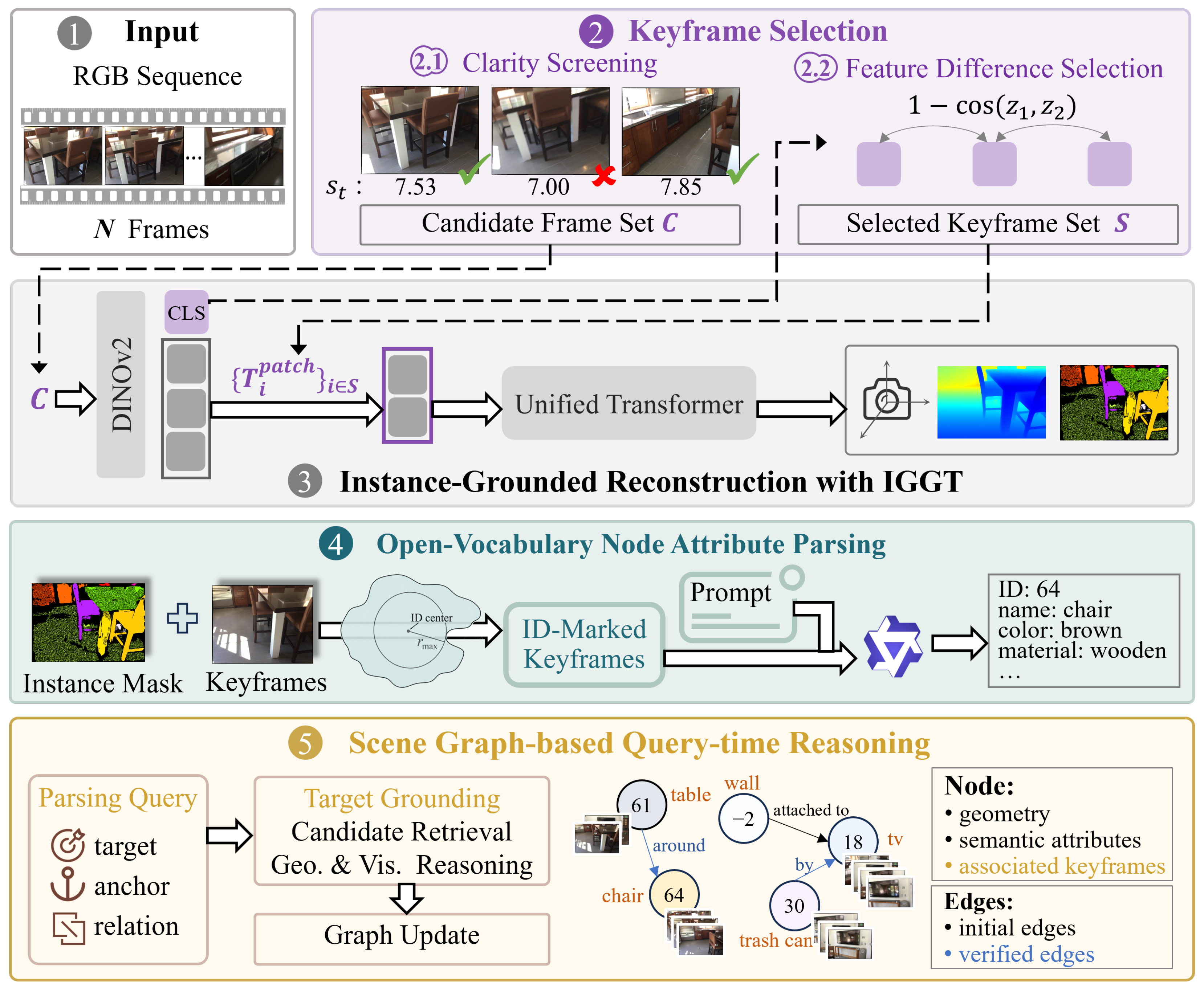
Figure 1.
Overview of KNA-SG. Given an RGB sequence, KNA-SG selects reliable keyframes, reconstructs object instances with IGGT, parses open-vocabulary node attributes from ID-marked keyframes, and organizes the resulting nodes and initial relations into a sparse 3D scene graph. At query time, structured geometric and visual reasoning is performed for object grounding, with verified relations written back to the graph. Dashed arrows indicate data-to-module associations.
Figure 1.
Overview of KNA-SG. Given an RGB sequence, KNA-SG selects reliable keyframes, reconstructs object instances with IGGT, parses open-vocabulary node attributes from ID-marked keyframes, and organizes the resulting nodes and initial relations into a sparse 3D scene graph. At query time, structured geometric and visual reasoning is performed for object grounding, with verified relations written back to the graph. Dashed arrows indicate data-to-module associations.
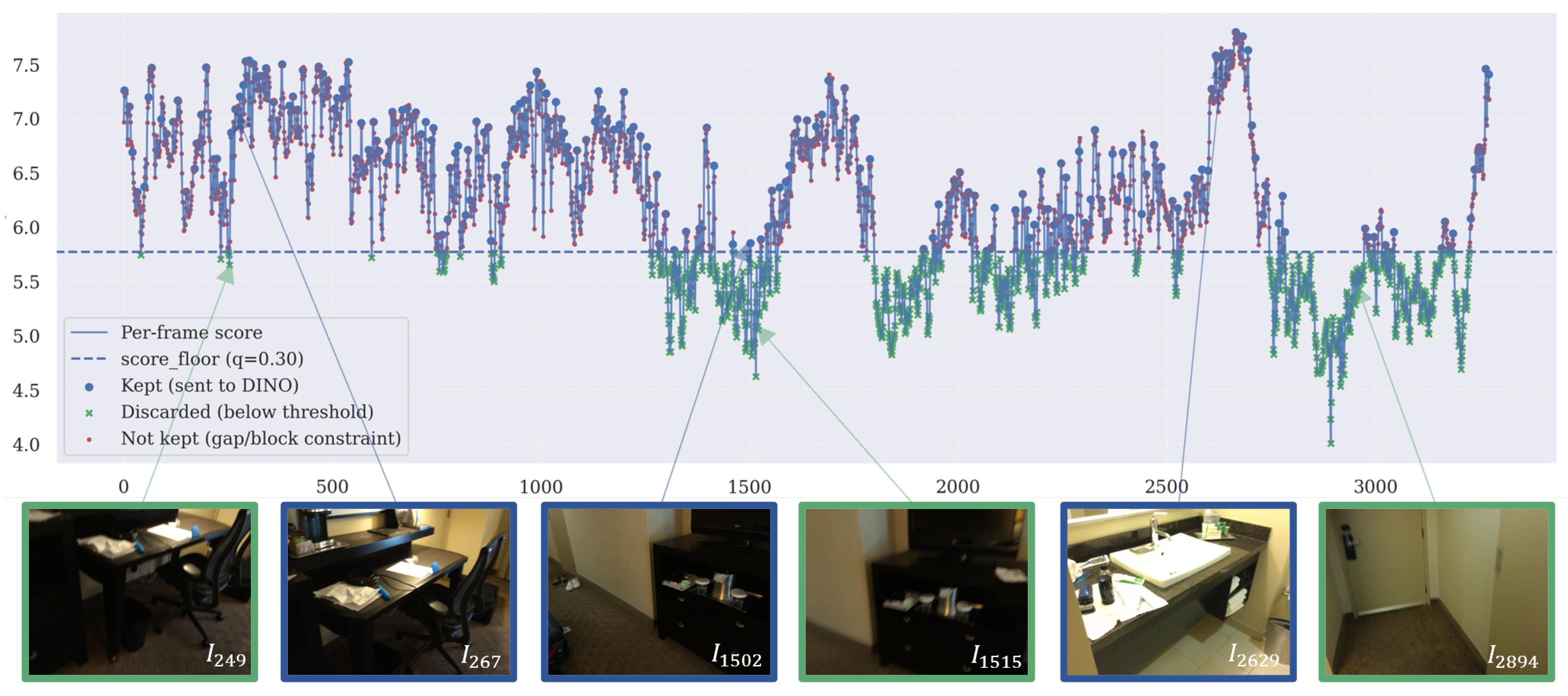
Figure 2.
Visualization of clarity-aware candidate selection on scene0046_00. The plot illustrates the per-frame clarity scores. Observations below the clarity threshold, such as and , are excluded before subsequent feature-based selection and multi-view reconstruction.
Figure 2.
Visualization of clarity-aware candidate selection on scene0046_00. The plot illustrates the per-frame clarity scores. Observations below the clarity threshold, such as and , are excluded before subsequent feature-based selection and multi-view reconstruction.
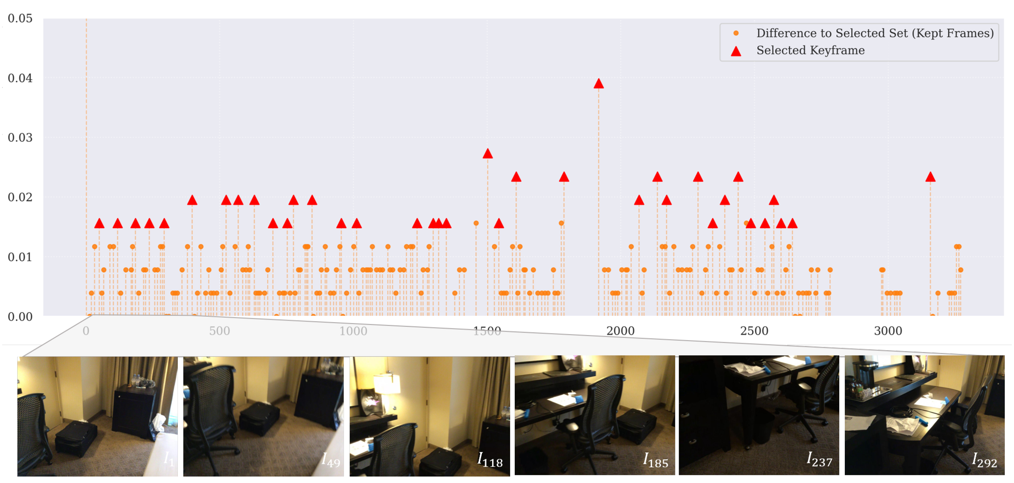
Figure 3.
Visualization of feature difference selection on scene0049_00. For each candidate frame, the feature difference is measured as its minimum cosine distance to the current selected keyframe pool in the DINOv2 global feature space. The triangles indicate the final retained keyframes.
Figure 3.
Visualization of feature difference selection on scene0049_00. For each candidate frame, the feature difference is measured as its minimum cosine distance to the current selected keyframe pool in the DINOv2 global feature space. The triangles indicate the final retained keyframes.
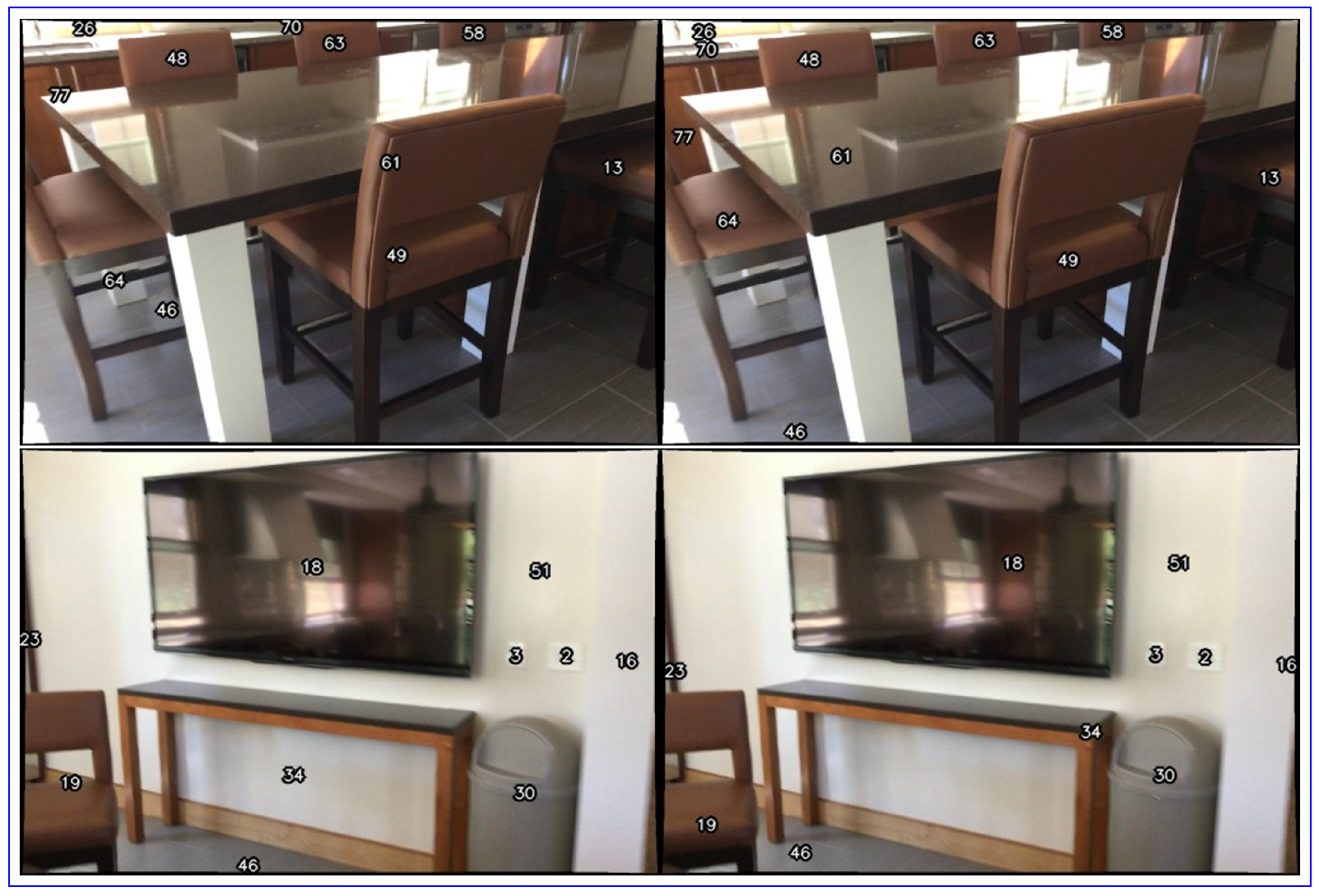
Figure 4.
Comparison of ID-mark placement strategies. The (left column) uses the center of the minimum bounding rectangle, where some ID marks may appear near object boundaries or even outside the visible object regions. The (right column) uses the center of the maximum inscribed circle, which places ID marks more stably inside the visible instance regions. The effectiveness of the two strategies can be compared via the annotated instances 19: “chair”, 34: “console table”, 61: “table”, 64: “chair”, and 77: “cabinet”.
Figure 4.
Comparison of ID-mark placement strategies. The (left column) uses the center of the minimum bounding rectangle, where some ID marks may appear near object boundaries or even outside the visible object regions. The (right column) uses the center of the maximum inscribed circle, which places ID marks more stably inside the visible instance regions. The effectiveness of the two strategies can be compared via the annotated instances 19: “chair”, 34: “console table”, 61: “table”, 64: “chair”, and 77: “cabinet”.
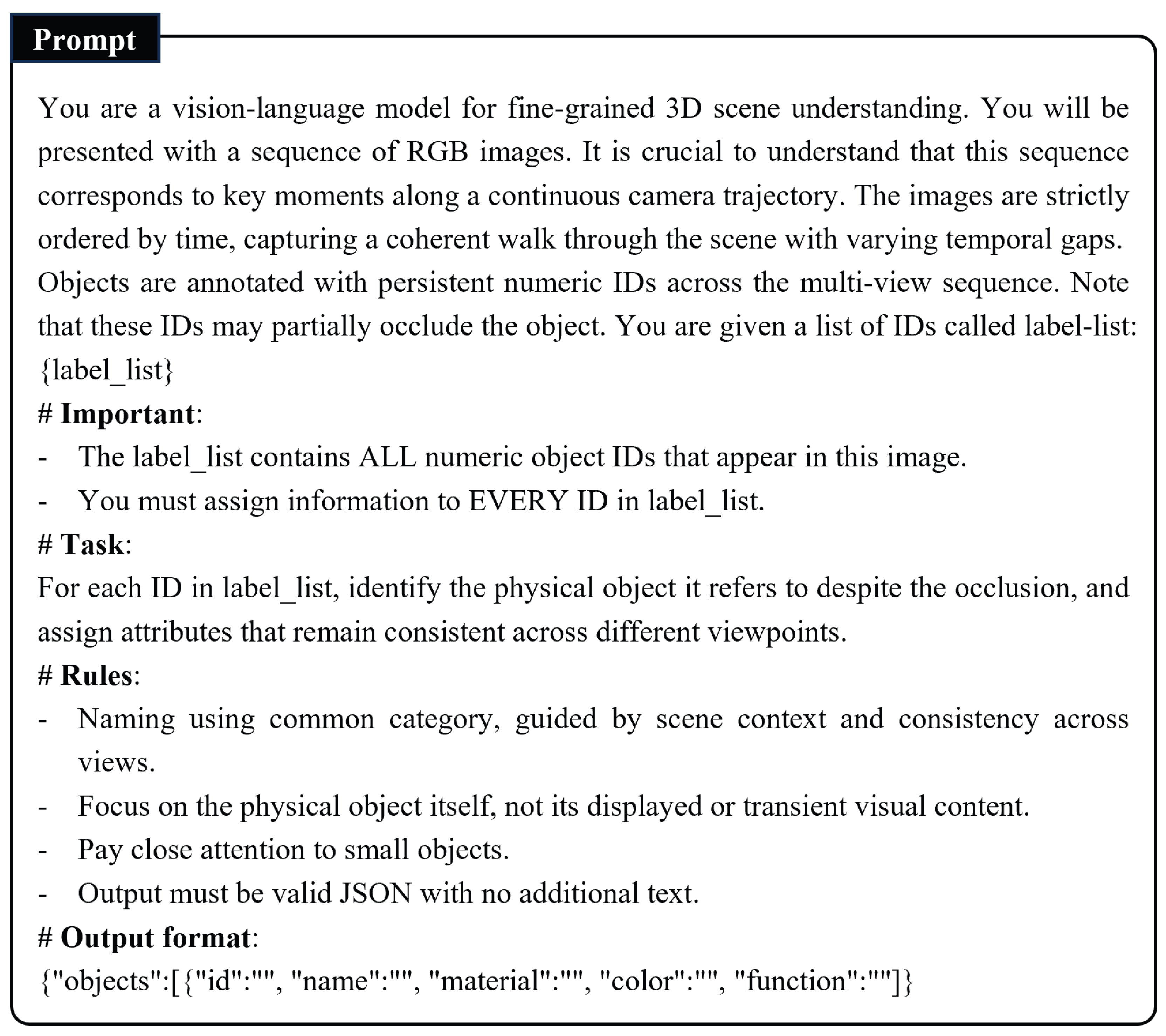
Figure 5.
Illustration of the task-specific prompt for ID-guided node parsing. The prompt instructs the MLLM to associate each rendered visual ID with the corresponding object instance and to output standardized semantic attributes. The parsed attributes are stored as structured node metadata for subsequent scene graph construction.
Figure 5.
Illustration of the task-specific prompt for ID-guided node parsing. The prompt instructs the MLLM to associate each rendered visual ID with the corresponding object instance and to output standardized semantic attributes. The parsed attributes are stored as structured node metadata for subsequent scene graph construction.
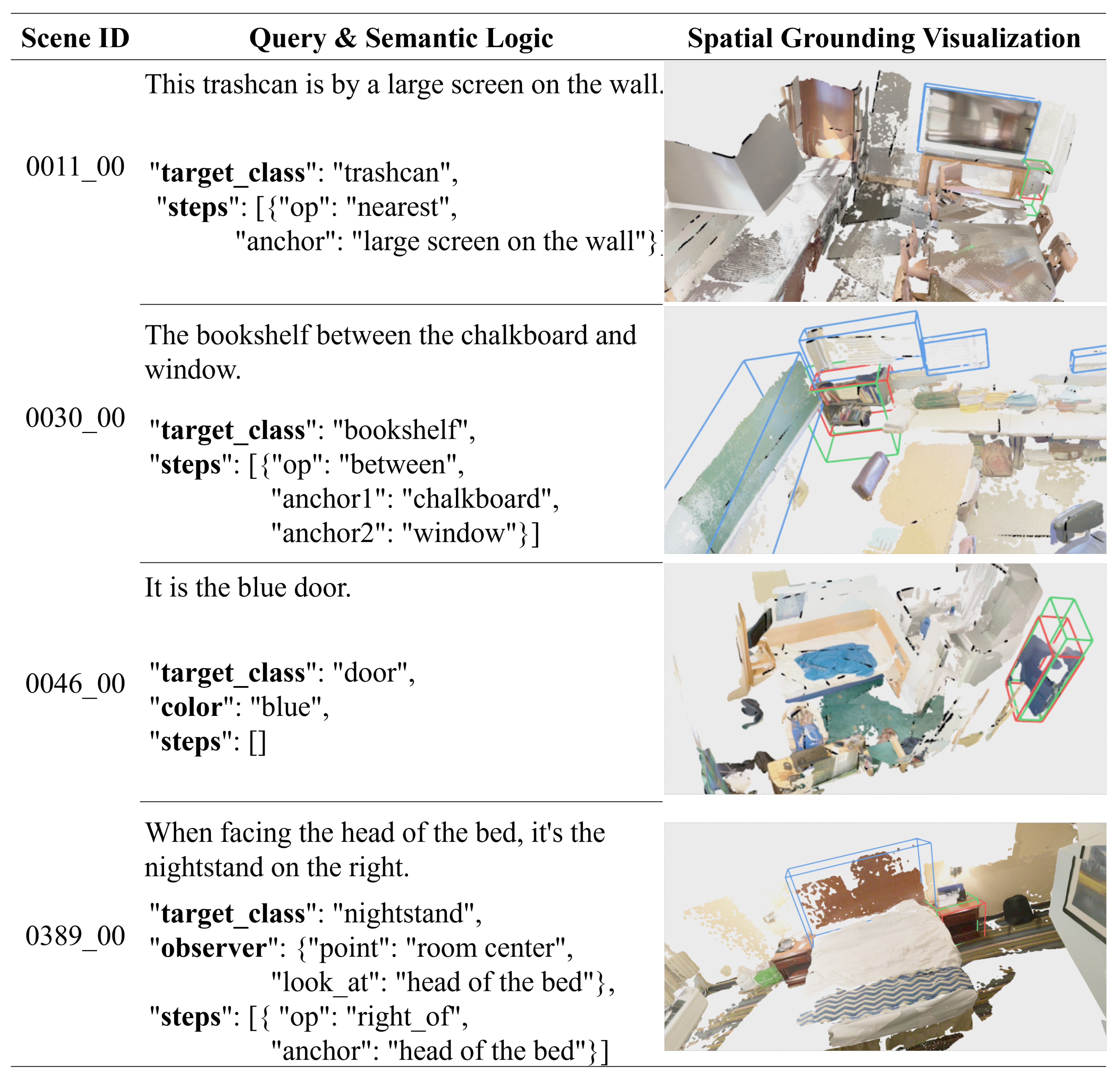
Figure 6.
Qualitative examples of language-guided target localization and semantic logic parsing on the NR3D dataset. The Query and Semantic Logic column displays the decomposition of instructions into executable spatial primitives. For orientation-sensitive predicates, the logic is resolved relative to the observer’s egocentric reference frame to achieve precise target localization. In the Grounding Visualization, the red, green, and blue bounding boxes denote the predicted target, ground truth (GT), and anchor objects, respectively.
Figure 6.
Qualitative examples of language-guided target localization and semantic logic parsing on the NR3D dataset. The Query and Semantic Logic column displays the decomposition of instructions into executable spatial primitives. For orientation-sensitive predicates, the logic is resolved relative to the observer’s egocentric reference frame to achieve precise target localization. In the Grounding Visualization, the red, green, and blue bounding boxes denote the predicted target, ground truth (GT), and anchor objects, respectively.
Table 1.
Quantitative comparison of open-vocabulary 3D semantic segmentation on Replica and ScanNet.
Table 1.
Quantitative comparison of open-vocabulary 3D semantic segmentation on Replica and ScanNet.
| Methods | Replica | ScanNet |
|---|
|
mAcc
|
mIoU
|
F-mIoU
|
mAcc
|
mIoU
|
F-mIoU
|
|---|
| ConceptGraphs [4] | 0.36 | 0.18 | 0.15 | 0.52 | 0.26 | 0.29 |
| HOV-SG [15] | 0.30 | 0.23 | 0.39 | 0.47 | 0.30 | 0.37 |
| Open3DSG [17] | 0.35 | 0.31 | 0.45 | 0.52 | 0.36 | 0.31 |
| BBQ-CLIP [5] | 0.38 | 0.27 | 0.48 | 0.56 | 0.34 | 0.36 |
| GaussianGraph [16] | 0.49 | 0.31 | - | 0.49 | 0.31 | - |
| Ours | 0.51 | 0.39 | 0.69 | 0.58 | 0.44 | 0.50 |
Table 2.
Language-guided 3D object grounding results on the Nr3D dataset. A@0.1 and A@0.25 denote grounding accuracy under 3D bounding-box IoU thresholds of 0.1 and 0.25, respectively.
Table 2.
Language-guided 3D object grounding results on the Nr3D dataset. A@0.1 and A@0.25 denote grounding accuracy under 3D bounding-box IoU thresholds of 0.1 and 0.25, respectively.
| Methods | Overall | Easy | Hard | View Dep. | View Indep. |
|---|
|
A@0.1
|
A@0.25
|
A@0.1
|
A@0.1
|
A@0.1
|
A@0.1
|
|---|
| ConceptGraph [4] | 16.0 | 7.2 | 18.7 | 9.1 | 12.7 | 17.0 |
| GaussianGraph [16] | 17.2 | 8.6 | 20.7 | 10.9 | - | - |
| BBQ [5] | 28.3 | 19.0 | 30.5 | 22.8 | 23.6 | 29.8 |
| Open3DSG [17] | 31.4 | 22.5 | 32.3 | 25.2 | 24.3 | 33.5 |
| KNA-SG | 43.8 | 29.2 | 50.4 | 26.9 | 37.6 | 45.7 |
Table 3.
Language-guided 3D object grounding results on the Sr3D dataset. A@0.1 and A@0.25 denote grounding accuracy under 3D bounding-box IoU thresholds of 0.1 and 0.25, respectively.
Table 3.
Language-guided 3D object grounding results on the Sr3D dataset. A@0.1 and A@0.25 denote grounding accuracy under 3D bounding-box IoU thresholds of 0.1 and 0.25, respectively.
| Methods | Overall | Easy | Hard | View Dep. | View Indep. |
|---|
|
A@0.1
|
A@0.25
|
A@0.1
|
A@0.1
|
A@0.1
|
A@0.1
|
|---|
| ConceptGraph [4] | 13.3 | 6.2 | 13.0 | 16.0 | 15.2 | 13.1 |
| GaussianGraph [16] | 18.2 | 7.4 | 19.1 | 16.3 | - | - |
| BBQ [5] | 34.2 | 22.7 | 34.3 | 33.3 | 32.9 | 34.4 |
| Open3DSG [17] | 37.3 | 25.8 | 36.5 | 36.1 | 36.1 | 36.6 |
| KNA-SG | 51.4 | 37.2 | 54.1 | 30.7 | 45.6 | 52.2 |
Table 4.
Ablation study of frame sampling strategies for object-level visibility coverage. MC denotes maximum-coverage sampling.
Table 4.
Ablation study of frame sampling strategies for object-level visibility coverage. MC denotes maximum-coverage sampling.
| Sampling Strategy | 3D Info | Obj@0.1 | SmallObj@0.1 | MeanCov |
|---|
| MC | Y | 100.00 | 100.00 | 86.21 |
| Uniform | N | 99.19 | 98.44 | 81.26 |
| Ours | N | 99.52 | 100.00 | 82.83 |
Table 5.
Ablation study of feature difference selection (FDS) on Replica.
Table 5.
Ablation study of feature difference selection (FDS) on Replica.
| FDS | mAcc | mIoU | F-mIoU |
|---|
| × | 41.62 | 29.85 | 66.40 |
| ✓ | 50.91 | 39.15 | 68.73 |
Table 6.
Ablation study of clarity-aware candidate selection (CCS) and feature difference selection (FDS) on ScanNet.
Table 6.
Ablation study of clarity-aware candidate selection (CCS) and feature difference selection (FDS) on ScanNet.
| CCS | FDS | mAcc | mIoU | F-mIoU |
|---|
| × | × | 54.10 | 39.67 | 45.85 |
| × | ✓ | 54.34 | 40.30 | 43.96 |
| ✓ | ✓ | 59.43 | 44.06 | 49.87 |
Table 7.
Effect of ID-based visual prompts on instance-level object perception. The “with ID” setting renders unique visual IDs on selected keyframes according to cross-view consistent instance masks, while the baseline uses raw RGB keyframes without explicit object references. Structural background categories are excluded. mIR denotes mean instance recall, and mCCS denotes mean count consistency score.
Table 7.
Effect of ID-based visual prompts on instance-level object perception. The “with ID” setting renders unique visual IDs on selected keyframes according to cross-view consistent instance masks, while the baseline uses raw RGB keyframes without explicit object references. Structural background categories are excluded. mIR denotes mean instance recall, and mCCS denotes mean count consistency score.
| Dataset | With ID | mIR | mCCS |
|---|
| Replica | × | 38.61 | 37.88 |
| ✓ | 51.31 | 47.42 |
| ScanNet | × | 47.96 | 40.36 |
| ✓ | 67.99 | 47.47 |
Table 8.
Ablation study of query execution strategies on the Nr3D dataset. A@0.1 denotes grounding accuracy under a 3D bounding-box IoU threshold of 0.1. Avg. Time reports the average inference time per query.
Table 8.
Ablation study of query execution strategies on the Nr3D dataset. A@0.1 denotes grounding accuracy under a 3D bounding-box IoU threshold of 0.1. Avg. Time reports the average inference time per query.
| Strategy | Overall | Easy | Hard | View Dep. | View Indep. | Avg. Time (s) |
|---|
| MLLM-based selection | 42.8 | 50.4 | 23.4 | 34.6 | 45.3 | 41.7 |
| Geometry-only reasoning | 37.3 | 44.6 | 18.8 | 31.5 | 39.1 | 9.6 |
| KNA-SG | 43.8 | 50.4 | 26.9 | 37.6 | 45.7 | 25.4 |