Article

Micro-Attention CNN Hybrid Architecture for Real-Time Stress Detection Using Minimalistic Bio-Signals

1
Multidisciplinary Faculty of Nador, Mohammed Premier University, Oujda 60000, Morocco
2
Laboratory LaSTI, ENSAK, Sultan Moulay Slimane University, Khouribga 23000, Morocco
*
Author to whom correspondence should be addressed.
Technologies 2026, 14(5), 300; https://doi.org/10.3390/technologies14050300
Submission received: 8 April 2026 / Revised: 4 May 2026 / Accepted: 11 May 2026 / Published: 13 May 2026
(This article belongs to the Special Issue AI-Enabled Smart Healthcare Systems)

Abstract

Real-time psychological stress detection on wearable and edge devices requires models that are accurate, computationally efficient, and small enough for on-device deployment. This paper proposes a Micro-Attention CNN Hybrid Architecture for stress recognition using wearable bio-signals. The model uses six sensor channels, namely tri-axial acceleration, electrodermal activity, heart rate, and skin temperature, and classifies three stress levels: no stress, low stress, and high stress. This study is conducted on a public wearable sensor dataset collected from 15 nurses during hospital work, providing a realistic benchmark for continuous stress monitoring under practical conditions. The proposed architecture combines one-dimensional and depthwise separable convolutions with a lightweight attention module to emphasize the most informative temporal patterns in short multivariate signal segments. To support deployment on resource-constrained devices, we further apply structured pruning, selective quantization-aware training, and post-training quantization. The full-precision model achieves a Macro-F1 score of 99.63%, while the final compressed model retains 98.03% Macro-F1 with a model size of 1.76 kilobytes and a CPU inference latency of 0.40 ms. Additional analyses show that most residual errors occur near the boundary between low stress and neighboring classes, while simple post-compression calibration improves reliability. These results demonstrate that accurate and low-latency stress detection using wearable bio-signals is feasible on compact edge hardware without transmitting raw sensor streams off-device.

1. Introduction

Psychological stress [1,2] is a pervasive driver of morbidity and diminished quality of life, shaping cognition, decision making, and physiological homeostasis [3]. As consumer wearables and clinical-grade sensors proliferate [4], there is growing interest in unobtrusive, continuous assessment that can surface early warnings and support timely self-regulation or clinical triage [5]. Physiological streams such as electrodermal activity (EDA) as a proxy for sympathetic arousal; cardiac measures including heart rate (HR), heart rate variability (HRV), and electrocardiography (ECG); peripheral temperature (TEMP); photoplethysmography (PPG); and tri-axial accelerometry (ACC) provide complementary views on autonomic reactivity and behavioral context [6]. Yet, these signals are noisy, nonstationary, and person-dependent; they drift with ambient conditions, are confounded by posture and movement, and reflect complex biopsychosocial mechanisms [7]. The central challenge is to translate heterogeneous, artifact-prone time series into reliable stress estimates that remain faithful under everyday conditions rather than only in controlled laboratory settings [8,9,10].
Data handling and labeling are pivotal in this translation. Real-world datasets often mix high-frequency physiological streams with irregular events, weak proxies of stress (for example, task epochs or self-reports), and heterogeneous taxonomies that vary across studies [11]. A principled pipeline typically begins with synchronized acquisition and basic hygiene (artifact mitigation, detrending, outlier handling), followed by normalization across sessions or individuals to reduce inter-subject variability. Windowing choices must respect physiological time scales and downstream compute budgets since the temporal granularity of segments constrains both what dynamics can be captured and the latency of any real-time system. Equally important is split discipline: train, validation, and test partitions should be established before any window generation to prevent identity or temporal leakage, and subjectwise protocols are essential when the goal is generalization to unseen users [12]. Class imbalance is the rule rather than the exception, motivating resampling strategies and balanced optimization, which prevent minority classes from being swamped during training [13].
Modeling choices span a spectrum from feature-based classical learning to end-to-end deep architectures. Hand-crafted descriptors (for example, tonic–phasic EDA decomposition, HRV features from inter-beat intervals, and spectral power in physiologically meaningful bands) [14] remain attractive for their interpretability and modest resource usage, especially when paired with linear models or tree ensembles. Deep approaches leverage 1D convolutions for local temporal patterns, recurrent or temporal-convolutional networks for longer dependencies, and attention mechanisms for context-sensitive weighting across channels and time [15]. Regardless of the paradigm, deployment on microcontroller-class hardware imposes tight constraints on latency, memory, and energy. This drives interest in model compression (structured pruning, low-rank factorization, weight clustering, knowledge distillation) [16,17], quantization-aware and post-training quantization [18], and kernel-level co-design that exploits device-specific SIMD or DSP instructions. The aim is not only to achieve strong accuracy but to do so within budgets that enable always-on operation without offloading raw bio-signals [19].
Evaluation therefore must extend beyond headline accuracy. Sound methodology distinguishes between subject-dependent and subject-independent settings [20], probes robustness under distribution shifts (for example, day-to-day variation, sensor repositioning, or activity contexts) [21], and reports confusion patterns that reveal asymmetric errors across stress strata. Calibration metrics such as expected calibration error are increasingly relevant when predictions inform behavioral nudges or clinical review; selective prediction or abstention mechanisms can further reduce harm by allowing models to defer when uncertainty is high [22]. For streaming, embedded use and end-to-end measurements—including sensor I/O, buffering, on-device preprocessing, and inference—are needed to quantify true latency and energy per decision, not just isolated forward-pass timings [23]. Finally, privacy, security, and fairness are first-class concerns: on-device inference limits data exposure; population-level learning can adopt federated or continual strategies with privacy-preserving updates; and audits should check for biases across demographics, occupations, and sensor contexts [24]. Taken together, these considerations define a rigorous pathway from raw wearable data to trustworthy, resource-aware stress monitoring that can operate quietly, locally, and respectfully in daily life.
In this paper, we present a Micro-Attention CNN Hybrid tailored to real-time stress detection from a compact 32 × 6 physiological window, combining efficient 1D and depthwise-separable convolutions with a lightweight micro-attention block that selectively emphasizes clinically informative segments. The network culminates in a compact classifier for globally pooled features, designed for sub-millisecond inference and kilobyte-scale memory on TinyML hardware. We pair this architecture with a leakage-aware preprocessing and evaluation pipeline and report comprehensive results, including calibration and boundary analyses, to illustrate readiness for embedded deployment.
The main contributions of this research are:
  • Kilobyte-scale TinyML with micro-attention. We introduce a Micro-Attention CNN Hybrid explicitly co-designed for edge deployment that achieves an 88% size reduction down to 1.76 KB with 0.40 ms CPU inference, bringing three-class stress recognition into the sub-2 KB regime, far smaller than prior on-device systems that typically occupy hundreds of kilobytes to megabytes. This substantially tightens the memory/latency envelope for real-time stress detection on microcontrollers.
  • Selective QAT that preserves attention/BN in full precision. We propose a selective quantization-aware training strategy that quantizes only convolutional and dense layers while intentionally keeping BatchNorm and the micro-attention block in FP32. This preserves the model’s capacity to focus on subtle, boundary-case physiology while still delivering the majority of the latency/size gains—a practical recipe for compressing attention-equipped TinyML models.
  • Biologically grounded, ultra-short windowing. We justify and use a compact 32 × 6 window at 32 Hz ( ACC x , y , z , EDA, HR, TEMP) that matches the time scale of acute stress responses yet remains compute-light, and we detail the end-to-end micro-attention hybrid that exploits this representation with only ∼3.8 K parameters. This balances physiological fidelity with TinyML constraints.
  • Leakage-aware resampling with neighborhood diagnostics. Beyond standard class rebalancing, we introduce a Δ NN , c neighborhood density check to verify that synthetic samples densify plausible regions without collapsing local structure, and we enforce leakage-safe splits before windowing. This provides a principled guardrail against distributional artifacts in highly imbalanced stress data.
  • Compression robustness and boundary analysis. We systematically characterize how pruning → selective QAT → PTQ affects classwise errors and show that residual mistakes concentrate at the low stress boundary, and then preserve high global performance after full compression. This offers rare, fine-grained evidence about ambiguity under aggressive model shrinking in stress recognition.
  • Deployment-oriented reporting. We report both accuracy and device-realistic metrics (model size and CPU latency) under each compression stage, enabling reproducible trade-off decisions for embedded practitioners targeting strict RAM/latency budgets.
The remainder of this paper is organized as follows: Section 2 reviews related works on TinyML-based stress recognition and positions our study within the field. Section 3 presents the proposed methodology, including our data pipeline, model design, and compression strategy. Section 4 reports the experimental results and analyses, covering evaluation protocols, baseline findings, compression outcomes, and ablation insights, as well as a discussion of limitations. Finally, Section 5 concludes this paper and outlines directions for future work.

2. Related Works

The deployment of intelligent stress detection systems on resource-constrained edge devices represents a significant advancement in personalized healthcare. This section reviews several pioneering studies that have successfully implemented TinyML models for real-time stress classification, showcasing a diverse range of approaches. These include variations in the physiological signals monitored, the machine learning architectures employed, and the specific hardware platforms targeted.
To begin, Rachakonda et al. [25] suggested a DNN-integrated edge device for real-time stress level detection within the Internet of Medical Things (IoMT). Their methodology centers on a Deep Neural Network (DNN) deployed on an edge device (a wearable wristband) that processes data from three physiological sensors: temperature, humidity (for sweat), and an accelerometer (for motion). The model was trained and tested using a combined dataset of 26,000 samples, built from real-life datasets like Human Motion Primitives (HMP) and the PAMAP2 Physical Activity Monitoring dataset, with sensor value ranges defined for stress classification. The system achieved a high accuracy between 98.3% and 99.7% across different tests, successfully validating the concept of on-device, real-time stress detection.
Building upon this concept with a focus on data security, Rachakonda et al. [26] proposed a blockchain-integrated privacy-assured IoMT framework for stress management that analyzes sleeping habits to predict next-day stress levels. Their methodology employs a Fully Connected Neural Network (FCN) deployed on an edge device (a smart pillow) to process physiological data such as heart rate, respiration, snoring, and body temperature during sleep, with all analyzed data securely stored and managed via a private Ethereum blockchain. The model was trained and tested using 15,000 samples from the National Sleep Research Resource (NSRR) dataset. The system achieved a high accuracy of 96% for stress prediction and successfully demonstrated a secure, privacy-preserving data storage and access mechanism using blockchain technology.
In parallel, adopting a strategy to enhance reliability, Gibbs et al. [27] presented a multimodal context-aware stress recognition system that combines two separate tinyML models on a single, resource-constrained microcontroller (Arduino Nano 33 BLE Sense) to improve reliability by mitigating motion artifacts. Their methodology employs two 1D Convolutional Neural Networks (CNNs): one for Human Activity Recognition (HAR) using accelerometer data to classify users as ’active’ or ’resting’, and a second for stress detection using heart rate and electrodermal activity data that is only triggered during periods of inactivity identified by the first model. The models were trained on the public WISDM dataset for activity recognition and a lab-collected dataset using the Montreal Imaging Stress Task for stress, and they were optimized for deployment using post-training quantization (int8 and float16). The results showed that the system successfully ran on the device, with the HAR and stress models achieving 98% and 88% accuracy respectively, validating a novel, privacy-preserving approach to real-time, context-aware stress detection.
Shifting the focus to a different physiological modality, Mai et al. [28] introduced an on-chip mental stress detection system that integrates a wearable behind-the-ear (BTE) EEG device with an embedded tiny Convolutional Neural Network (CNN). Their methodology involves capturing single-channel BTE EEG signals, performing on-chip noise removal and Fast Fourier Transform (FFT)-based signal-to-spectrogram conversion, and classifying stress levels using a compact, quantized CNN model deployed on a microcontroller. The dataset was collected from 15 participants undergoing stress-inducing tasks (Stroop and Mental Arithmetic), resulting in spectrogram images labeled as stress or non-stress. The system achieved high performance, with 95.32% accuracy using 10-fold cross-validation and 91.72% using leave-one-out cross-validation, while maintaining low power consumption and real-time processing capabilities.
Likewise, concentrating on another popular physiological signal, Rostami et al. [29] developed a real-time stress detection system using a Long Short-Term Memory (LSTM) deep learning model optimized for deployment on resource-constrained microcontrollers via TinyML. Their methodology involved training an LSTM network directly on raw, unprocessed photoplethysmography (PPG) signals from the WESAD dataset, using sliding window segmentation, and then applying model compression techniques, including pruning and post-training quantization, to reduce its size and memory requirements. The optimized model achieved an accuracy of 87.76% on the test set while requiring only 170 KB of RAM, enabling efficient real-time inference on low-power STM32 microcontrollers.
Finally, demonstrating the effectiveness of traditional ML models on ultra-constrained hardware, Abu Samah et al. [19] designed a TinyML-based stress classification system using a multi-sensor wearable device built around a Raspberry Pi Pico RP2040 microcontroller. Their methodology involved training and comparing several traditional machine learning models on a public dataset of nurses’ physiological data, including acceleration, body temperature, heart rate, and electrodermal activity, using hyperparameter tuning and NearMiss undersampling to handle class imbalance. The optimized XGBoost model achieved 86.0% accuracy for three-class stress detection (no stress, low stress, and high stress) and was successfully deployed on the resource-constrained edge device, occupying only 1.12 MB of flash memory.
Compared with existing TinyML stress detectors, our research advances the state of the art along four practical axes for embedded deployment. (1) Kilobyte-scale model and sub-millisecond latency: Through a staged pipeline (structured pruning → selective QAT → PTQ), our final artifact operates at 1.76 KB with 0.40 ms CPU latency while retaining 98.03% Macro-F1, tightening the memory/latency envelope substantially versus prior on-device systems that either do not report such ultra-small footprints or remain in the hundreds-of-kilobytes range. (2) Micro-attention under selective quantization: We integrate a lightweight self-attention block and explicitly preserve attention and batch-normalization layers in FP32 during QAT to protect boundary sensitivity while still reaping most compression gains, an implementation detail seldom surfaced in prior TinyML stress works. (3) Biologically grounded, ultra-short windowing: The model consumes a 32 × 6 (≈1 s at 32 Hz) multimodal window ( ACC x , y , z , EDA, HR, TEMP) that captures acute stress dynamics while staying compute-light for MCUs. (4) Deployment-oriented validation knobs: Beyond accuracy, we analyze compression-stage effects on near-boundary errors (notably in low stress) and show that boundary-aware calibration can recover F1 and push ECE below 0.5% without changing the footprint, offering neutral “safety dials” missing in most embedded reports.
Table 1 situates our system relative to TinyML stress detectors spanning DNN/FCN/CNN/LSTM/Boosted-tree approaches and multiple sensing stacks. In short, (a) prior MCU deployments rarely report both latency and footprint at the kilobyte scale; (b) several emphasize privacy frameworks or context gating but stop short of sub-ms inference or boundary calibration; and (c) RAM/flash budgets are often ≫100 KB, whereas our design demonstrates 1.76 KB with maintained three-class performance.

3. Proposed Methodology

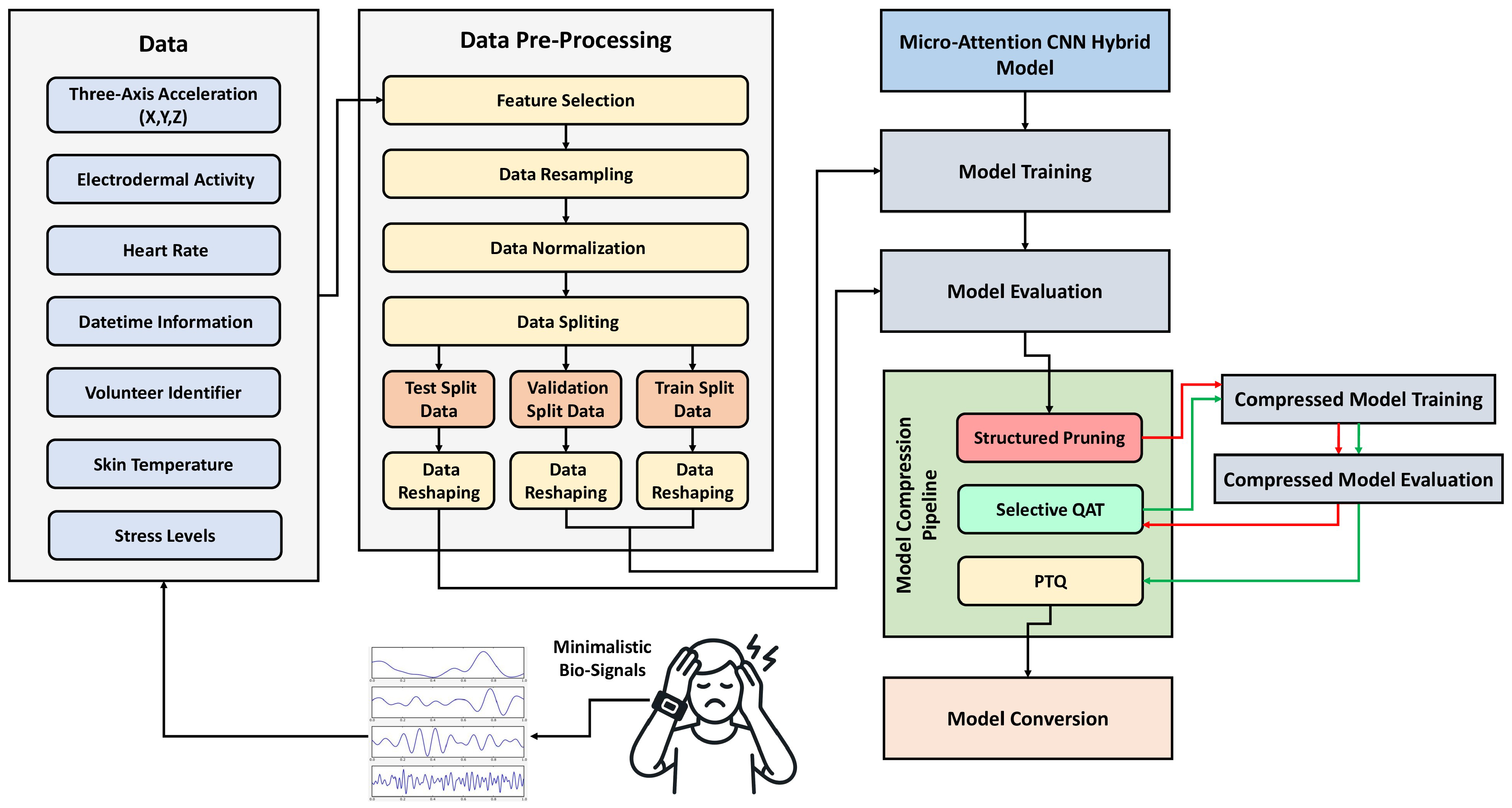
This section presents our comprehensive framework for developing and optimizing an efficient stress detection system. We introduce a novel Micro-Attention CNN Hybrid Architecture specifically designed for processing minimalistic bio-signals, accompanied by a detailed data preprocessing pipeline and an advanced model compression strategy. The methodology encompasses the entire workflow from raw data preparation to model optimization for edge deployment, addressing both algorithmic efficiency and practical implementation constraints for real-time stress monitoring applications. Figure 1 shows an overview of our proposed methodology.

3.1. Data Description

The analysis is based on the Nurse Stress Prediction Wearable Sensors dataset, a merged CSV file publicly available on Kaggle [30]. This dataset originates from a study designed for continuous stress monitoring of 15 volunteer nurses in a hospital setting during the COVID-19 outbreak. The compiled dataset is substantial, containing roughly 11.5 million data points structured in nine columns. The recorded variables encompass three-axis acceleration, EDA, HR, TEMP, a unique volunteer identifier (id), precise date–time information, and a target variable indicating three distinct stress levels: no stress, low stress, and high stress. An excerpt from the dataset illustrating multivariate physiological time-series data is presented in Table 2.

3.2. Data Preprocessing

To enhance data quality and ensure optimal classification performance, we applied a structured preprocessing pipeline. We treat the raw corpus as a labeled multivariate time–series collection indexed by participant and time, then constrain learning to physiologically meaningful channels by removing administrative attributes. Let the full dataset be the big union over subjects and their discrete time indices
D = s = 1 S t T s x s , t , y s , t ,
where S denotes the number of participants, T s the index set of timestamps for participant s, x s , t R p the raw feature vector at time t, and y s , t { 0 , 1 , 2 } the stress class label. We apply a pointwise feature-selection map ϕ : R p R 6 that removes participant identifiers and timestamps while retaining the physiologically relevant channels as follows:
z s , t : = ϕ ( x s , t ) = X s , t , Y s , t , Z s , t , EDA s , t , HR s , t , TEMP s , t R 6 .
This restriction prevents shortcut learning via non-physiological fields and focuses the hypothesis class on kinematics (three axes) and autonomic markers (electrodermal activity, heart rate, temperature) that carry a mechanistic signal for stress.

3.2.1. Class Imbalance and Two-Stage Resampling (See Figure 2)

The dataset is highly imbalanced with counts ( n 0 , n 1 , n 2 ) = (2,162,246, 806,222, 8,540,583) and total N = c = 0 2 n c . We quantify skew using the empirical prevalence vector π = ( π 0 , π 1 , π 2 ) with
π c = n c N , c { 0 , 1 , 2 } ,
and the imbalance ratio
IR = max c n c min c n c = 8,540,583 806,222 10.60 ,
which indicates a dominant head class ( c = 2 ). We therefore adopt a hybrid policy: (i) random undersampling of class 2 to a cap U = 4,000,000 , and (ii) SMOTE oversampling [31] for classes 0 and 1. For stage (i), if I 2 indexes class 2 instances, we draw without replacement a uniform subset J 2 I 2 with | J 2 | = U and keep { ( z i , 2 ) : i J 2 } . For stage (ii), letting T c be the target size for minority class c { 0 , 1 } and s c = max { 0 , T c n c } the oversampling budget, each synthetic point is generated by convex interpolation along a within-class local segment as follows:
z ˜ = z i + λ z NN ( i ) z i , λ U [ 0 , 1 ] , y ˜ = c ,
where z i is a minority seed and z NN ( i ) one of its k-nearest minority neighbors in R 6 under Euclidean distance. After resampling, we denote N 2 = U and N c = n c + s c for c { 0 , 1 } , induce prevalences π c = N c / k N k , and track balance via the KL divergence from the uniform prior u = ( 1 / 3 , 1 / 3 , 1 / 3 ) as follows:
D KL π u = c = 0 2 π c log π c 1 / 3 ,
which decreases as classes equalize. This two-stage scheme reduces the dominance of the head class while densifying minority manifolds in physiologically plausible regions, improving sample efficiency and mitigating bias–variance pathologies associated with one-sided strategies.
Figure 2. Data resampling steps.
Technologies 14 00300 g002

3.2.2. Design of Targets and Equivalence to Loss Weighting

Choosing ( U , T 0 , T 1 ) can be guided by a risk-theoretic objective. For a K-class loss and model f θ , the empirical risk under class-conditional sampling with class weights w = ( w 0 , , w K 1 ) is
L w ( θ ) = c = 0 K 1 w c 1 M c i B c l f θ ( Z i ) , c ,
where B c collects batch indices with label c and M c = | B c | . If we resample to achieve class proportions π ^ c in mini-batches while using uniform weights w c = 1 , then in expectation,
E L unif ( θ ) = c π ^ c E l ( f θ ( Z ) , c ) | Y = c ,
which matches the effect of weighting with w c 1 / π c when π ^ c 1 / K . Hence, ( U , T 0 , T 1 ) can be chosen to target a desired effective weighting without introducing explicit class weights; we exploit this to simplify optimization while preserving calibration on natural prevalences by evaluating on the untouched test set.

3.2.3. Leakage Control and Temporal Integrity

To avoid optimistic bias, all resampling and neighborhood computations occur strictly within the training split; validation and test retain their natural distributions. Denote the post-split sets by I tr , I val , I te . The no-leakage constraint can be written as
c supp SMOTE c ( I tr ) I val I te = ,
which we enforce by fitting neighbors and generating z ˜ only from I tr and by windowing after splitting so that temporal segments never straddle set boundaries.

3.2.4. Normalization Across Heterogeneous Channels [32]

We normalize features using statistics fitted on the training set to harmonize scales and stabilize optimization. For each channel j { 1 , , 6 } with training mean μ j and standard deviation σ j > 0 , the standardization map is
Norm ( z ) = ( z 1 μ 1 ) / σ 1 , , ( z 6 μ 6 ) / σ 6 ,
and the same ( μ j , σ j ) values are reused for validation and test. Under heavy-tailed noise, we can substitute medians m j and interquartile ranges IQR j to obtain the robust transform ( z j m j ) / IQR j with an identical downstream interface. Conditioning of the optimization problem improves as feature covariance approaches identity; writing Σ ^ for the empirical covariance of normalized features and κ ( Σ ^ ) for its spectral condition number, standardization aims to reduce
κ ( Σ ^ ) = λ max ( Σ ^ ) λ min ( Σ ^ ) ,
thereby yielding more uniform gradient scales across channels and faster, stabler convergence.

3.2.5. Stratified Partitioning

We split the postprocessed dataset into disjoint index sets I tr , I val , I te with proportions ( 0.70 , 0.15 , 0.15 ) , preserving class priors after resampling and confining all resampling to the training split. Writing empirical frequencies per split, stratification enforces
| { i I tr : y i = c } | | I tr | | { i I val : y i = c } | | I val | | { i I te : y i = c } | | I te | π c ,
so that validation and test remain representative and unbiased for final evaluation, while normalization parameters are estimated only on I tr to eliminate leakage. When the evaluation goal is cross-participant generalization, a subjectwise variant partitions at the participant level and preserves per-subject label histograms to ensure identity separation.

3.2.6. Temporal Reshaping and Many-to-One Supervision

We reshape features into overlapping windows of L = 32 consecutive timesteps with F = 6 channels, yielding tensors of shape ( , 32 , 6 ) , where “−” is the batch dimension determined by the number of windows produced. For each participant s with standardized stream { z s , t } t T s and stride r N (typically r = 1 ), the window–label pairs are
Z s , τ = z s , t τ , z s , t τ + 1 , , z s , t τ + L 1 R L × F , y ˜ s , τ = y s , t τ + L 1 ,
implementing many-to-one supervision anchored at the terminal timestep. Windows never cross subject boundaries and are created after splitting to prevent temporal or identity leakage across sets. Because temporal persistence can alter the window-level class mixture, if m c counts windows with y ˜ = c , we monitor
π ^ c = m c k = 0 2 m k ,
and regulate exposure by tuning r or by class-balanced mini-batch sampling when necessary. The expected number of windows for subject s is
N s = max 0 , | T s |     L + 1 for r = 1 , N s = | T s |     L r + 1 in general ,
which controls the effective sample size and the correlation structure of batches via the overlap parameter r.
The choice of a 1 s analysis window reflects a deliberate trade-off between physiological fidelity and real-time embedded deployment. We agree that several stress-related physiological processes, especially tonic changes in electrodermal activity and temperature, can evolve over longer time scales than one second. However, the objective of the present system is not to estimate long-horizon autonomic trends from a single isolated segment but to provide low-latency stress recognition from short, continuously updated wearable measurements. In this setting, a 1 s window is long enough to capture rapid local variations in motion, heart rate behavior, and short-term electrodermal fluctuations, while remaining short enough to support frequent updates, reduced memory use, and very low inference latency on edge hardware. Moreover, the model operates on successive windows rather than a single one-shot segment, so slower physiological dynamics are still reflected across consecutive decisions over time. We therefore selected the 1 s window as a practical compromise that preserves short-term stress-sensitive information while remaining compatible with the strict computational constraints targeted in this work. A multi-scale extension that combines short and longer temporal contexts is an important direction for future research.

3.2.7. Optimization-Facing View and Gradient Variance

Let f θ : R L × F R K be the network and the loss (e.g., cross-entropy). For a mini-batch B with class-specific index sets B c = { i B : y ˜ i = c } , the empirical risk and its gradient read
L ( θ ) = c = 0 2 1 | B c | i B c l f θ ( Z i ) , c ,
θ L ( θ ) = c = 0 2 1 | B c | i B c θ f θ ( Z i ) f l .
Balancing classes renders the denominators | B c | comparable; normalization moderates the scale of θ f θ across channels; and windowed supervision supplies short-range dynamics aligned with labels. A convenient scalar diagnostic of training stability is the class-decomposed gradient variance
Var θ L ( θ ) c = 0 2 1 | B c | Var i B c θ f θ ( Z i ) f l ,
which decreases as | B c | equalizes and feature scales are harmonized, translating into steadier optimization and improved generalization.

3.2.8. Robustness Diagnostics

To validate that resampling leaves decision boundaries well posed, we check two post hoc criteria on the training split: (i) minority manifold connectedness by inspecting average intra-class k-NN distances before/after SMOTE,
Δ NN , c = 1 n c i : y i = c 1 k j NN k ( i ) z i z j 2 after · before ,
and (ii) prior-shift robustness by verifying that calibration under natural prevalences holds on the untouched test set. When Δ NN , c is small and non-negative, synthetic samples densify plausible regions without collapsing neighborhoods; when large and negative, we increase k or reduce s c to avoid over-concentration.

3.3. Introducing the Proposed Model

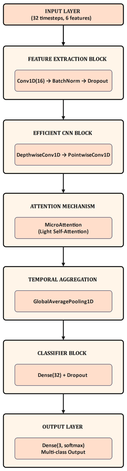
We proposed a novel Micro-Attention CNN Hybrid Architecture specifically designed for real-time stress detection using minimalistic bio-signals. The architecture begins with efficient 1D convolutional layers that extract localized temporal patterns from raw physiological signals, complemented by batch normalization and dropout for robust training. The core innovation lies in the integration of a micro-attention mechanism that selectively focuses on clinically relevant temporal segments within the bio-signals, enabling the model to identify subtle stress indicators without computational overhead. This hybrid approach combines the spatial efficiency of depthwise separable convolutions with the contextual awareness of attention, making it particularly suitable for resource-constrained wearable devices. The architecture culminates in a compact classifier that operates on globally pooled features, ensuring minimal latency for real-time inference. Figure 3 presents the architecture of our proposed model. Table 3 shows the detailed architecture of our model. The subsections below provide a detailed description of each architectural block in our proposed model.

3.3.1. Input Layer

The input layer is designed to process multivariate physiological time-series data with a specific temporal window of 32 consecutive timesteps, each containing 6 distinct bio-signal features. Mathematically, this is represented as X R b a t c h _ s i z e × 32 × 6 , where the dimensions correspond to the batch size, temporal length, and feature dimensionality, respectively. The 32-timestep window captures approximately one second of data at a 32 Hz sampling rate, which is optimal for detecting short-term stress patterns while maintaining computational efficiency. The six input features comprise three-axis accelerometer data (X, Y, Z) capturing physical movements and tremors, EDA measuring skin conductance responses, HR monitoring cardiovascular activity, and TEMP tracking peripheral thermal variations. This specific window size and feature selection are biologically grounded, as stress responses typically manifest within this temporal scale through measurable physiological changes including increased heart rate variability, elevated electrodermal activity, and characteristic movement patterns associated with anxiety states.

3.3.2. Feature Extraction Block

The feature extraction block employs a one-dimensional convolutional layer with 16 filters and kernel size 3, followed by batch normalization and dropout regularization. The convolutional operation is mathematically defined as Z [ t , k ] = i = 1 3 j = 1 6 W [ i , j , k ] × X [ t + i 1 , j ] + b [ k ] , where W R 3 × 6 × 16 represents the learnable convolutional kernels that slide across the temporal dimension to detect local patterns. The ReLU activation function A = max ( 0 , Z ) introduces non-linearity while maintaining computational efficiency. Batch normalization follows the convolution, implementing the transformation BN ( Z ) = γ ( ( Z μ B ) / σ B 2 + ε ) + β , which stabilizes training by normalizing activations and reducing internal covariate shift. A dropout rate of 0.2 is applied, mathematically represented as A drop = A M , where M is a binary mask with P ( M [ i ] = 1 ) = 0.8 , providing regularization by preventing co-adaptation of feature detectors. This sequential processing enables the model to extract locally invariant temporal patterns from the bio-signals while maintaining robustness to training instabilities.

3.3.3. Efficient CNN Block

The efficient CNN block implements depthwise separable convolution, which factorizes the standard convolutional operation into two distinct phases for enhanced computational efficiency. The depthwise convolution applies independent temporal filtering to each input channel through D d e p t h [ t , c ] = i = 1 5 W d e p t h [ i , c ] × A d r o p [ t + i 2 , c ] + b d e p t h [ c ] , where W d e p t h R 5 × 16 operates on 5-timestep windows across the 16 input channels. This is followed by pointwise convolution, which performs channel mixing through D p o i n t [ t , k ] = c = 1 16 W p o i n t [ c , k ] × D d e p t h [ t , c ] + b p o i n t [ k ] using W p o i n t R 16 × 32 . This factorization achieves a substantial parameter reduction from 2560 parameters in a standard convolution to only 592 parameters, representing a 76.9% decrease while maintaining representational capacity. The biological rationale for this design is that stress patterns manifest through both frequency-domain characteristics in individual bio-signals (captured by depthwise convolution) and complex interactions between different physiological modalities (captured by pointwise convolution), making this decomposition particularly suitable for multimodal stress detection.

3.3.4. Micro-Attention Mechanism

The micro-attention mechanism implements a lightweight self-attention module that enables the model to dynamically focus on clinically relevant temporal segments within the physiological signals. The process begins with linear projections that generate query (Q), key (K), and value (V) matrices through Q = W q × D p o i n t , K = W k × D p o i n t , and V = W v × D p o i n t , where W q , W k R 1 × 32 × 8 and W v R 1 × 32 × 32 are learnable projection matrices. The attention computation follows the scaled dot-product formulation Attention ( Q , K , V ) = softmax ( Q × K ) / d k × V , where d k = 8 represents the dimension of the key vectors and the scaling factor d k prevents gradient vanishing during training. The Softmax operation generates attention weights A [ t , u ] = exp ( S [ t , u ] / 8 ) / v = 1 32 exp ( S [ t , v ] / 8 ) , which represent the relative importance of each timestep when processing the current temporal context. This mechanism allows the model to identify and emphasize stress-indicative patterns such as sudden EDA surges or HRV depressions while attenuating irrelevant background physiological noise.

3.3.5. Temporal Aggregation

The temporal aggregation layer employs global average pooling to reduce the temporal dimensionality while preserving the most salient feature information. This operation is mathematically defined as G [ k ] = 1 32 t = 1 32 C [ t , k ] for k = 1 , , 32 , where C represents the output from the attention mechanism. This transformation reduces the tensor from dimensions R b a t c h × 32 × 32 to R b a t c h × 32 , achieving a significant parameter reduction in subsequent layers while maintaining the channelwise feature information. The global average pooling provides inherent translation invariance, making the model robust to temporal shifts in stress manifestations within the analysis window. From a physiological perspective, this operation computes the average activation for each feature channel across the entire temporal sequence, effectively capturing the overall intensity and persistence of stress-related patterns while discarding precise temporal localization that may be less critical for final stress state classification.

3.3.6. Classifier Block

The classifier block consists of a fully connected layer with 32 units followed by dropout regularization, serving as the primary decision-making component of the architecture. The dense layer operation is defined as H = ReLU ( W f c × G + b f c ) , where W f c R 32 × 32 represents the weight matrix and b f c R 32 the bias vector, implementing a non-linear transformation that learns complex interactions between the temporally aggregated features. The ReLU activation function introduces non-linearity while maintaining computational efficiency and mitigating the vanishing gradient problem. A dropout rate of 0.3 is applied through H d r o p = H M c l a s s , where M c l a s s is a binary mask with P ( M c l a s s [ i ] = 1 ) = 0.7 , providing robust regularization by preventing complex co-adaptations between neurons. This layer integrates the abstract representations learned from multiple bio-signal modalities, enabling the model to capture the complex, non-linear relationships between different physiological stress indicators such as the correlation between increased electrodermal activity and heart rate acceleration.

3.3.7. Output Layer

The output layer performs the final classification through a dense layer with 3 units and softmax activation, mathematically represented as y ^ = softmax ( W o u t × H d r o p + b o u t ) , where W o u t R 3 × 32 and b o u t R 3 . The softmax function is defined as softmax ( z i ) = e z i / j = 1 3 e z j , which normalizes the output into a probability distribution over three stress classes: no stress (class 0), moderate stress (class 1), and high stress (class 2). The final prediction is determined by the argmax operation, selecting the class with the highest probability. This output configuration provides clinically interpretable results that align with standard stress assessment protocols, while the probabilistic nature of the outputs enables confidence estimation and potential integration with decision support systems for real-time stress monitoring applications in educational and clinical settings.

3.4. Model Compression

This paper implements advanced model compression techniques to optimize the neural network for deployment on resource-constrained edge devices. The compression pipeline systematically reduces model size and computational requirements while maintaining detection accuracy for real-time stress monitoring applications.

3.4.1. Structured Pruning

We adopt structured pruning [16] to excise entire architectural components like filters, channels, and neurons, thereby delivering real reductions in parameters, activation sizes, and FLOPs, in contrast to unstructured sparsity, which zeroes isolated weights without guaranteed runtime gains. Consider a convolutional layer l mapping R C l × H × W R C l + 1 × H × W with m l = C l + 1 output filters; each filter k { 1 , , m l } is a tensor W l ( k ) R C l × K × K flattened into n l = C l K 2 scalars. We compute a magnitude-based importance for each filter as the mean absolute weight as follows:
I l ( k ) = 1 n l i = 1 n l | W l ( k , i ) | .
This choice approximates the l 1 norm per filter and promotes groupwise sparsity akin to a group-Lasso penalty while remaining training-framework-agnostic. Other monotone surrogates (e.g., l 2 norm or batch-normalization scale magnitudes) are compatible; the ranking they induce is typically similar in practice.
Given a per-layer target sparsity s l [ 0 , 1 ) and m l filters, we select the bottom s l m l filters by a thresholding rule. Let { I l ( 1 ) , , I l ( m l ) } be the set of importances and define the hard mask for each filter as
M l ( k ) = 0 , I l ( k ) < τ l , 1 , otherwise ,
where the per-layer threshold τ l is chosen as the empirical s l -quantile of importances as follows:
τ l = quantile { I l ( 1 ) , I l ( 2 ) , , I l ( m l ) } , s l .
The quantile operation ensures that approximately a fraction s l of the filters satisfies I l ( k ) < τ l and is thus set to zero, subject to implementation safeguards such as keeping at least one filter per layer to preserve connectivity. Aggregating decisions across layers defines the pruned index family P = ( l , k ) : M l ( k ) = 0 and its complement of survivors S = ( l , k ) : M l ( k ) = 1 , with the network-wide pruned set written as a big union over the layers as follows:
P = l = 1 L k { 1 , , m l } : I l ( k ) < τ l .
To avoid abrupt capacity collapse, we schedule sparsity over training using a third-order polynomial decay from an initial ratio s i to a final ratio s f over t end pruning steps, as follows:
s l ( t ) = s f + s i s f 1 t t end 3 , 0 t t end .
This schedule satisfies boundary conditions s l ( 0 ) = s i and s l ( t end ) = s f , is smooth with a vanishing slope at t = t end , and concentrates more pruning early when redundancy is high while tapering later to protect stabilized representations. In practice, we update τ l at discrete pruning events using the current importances and set s l to the scheduled value; between events, masks remain fixed.
At inference and during masked training, forward propagation applies binary masks at the group level. For convolutional filters, the masked kernel tensor at layer l is obtained by broadcasting the filterwise mask across all kernel entries as follows:
W l pruned = W l M l ,
where M l { 0 , 1 } m l × C l × K × K has entries ( M l ) k , : , : , : = M l ( k ) so that entire filters are either retained or nullified. The same construction extends to channel pruning (masking input channels) or neuron pruning in fully connected layers by broadcasting along the appropriate axis.
Backpropagation differentiates through masked weights using a straight-through estimator (STE) so that gradients flow only through surviving structures, as follows:
L W l = L W l pruned M l .
This identity reflects that W l pruned = W l M l , with M l treated as constant during the backward pass; masked groups ( M l ( k ) = 0 ) receive zero gradient and remain inactive, while active groups update normally. When pruning is performed iteratively, we recompute importances on the current W l (not W l pruned ), apply the schedule to increase s l , and refresh masks.
A central motivation for structured pruning is tangible efficiency. Writing the convolutional FLOPs for layer l (counting multiply–adds) as
FLOPs l = 2 H l W l C l K l 2 m l ,
and pruning a fraction s l of output filters yields an expected reduction
Δ FLOPs l 2 H l W l C l K l 2 s l m l ,
and the surviving cost scales linearly with ( 1 s l ) m l . If we prune input channels instead, the same formula holds with C l replaced by ( 1 s l 1 ) m l 1 , showing how upstream pruning compounds savings downstream by shrinking both weight tensors and activation maps. This translates directly into memory and latency benefits on hardware kernels that exploit contiguous channel layouts.
We also monitor the stability of the pruning signal and its effect on calibration. Let I l ( t ) and I l ( t + Δ ) be the rank orderings of filter importances at two pruning events; Kendall’s τ provides a concordance score of
τ l = # concordant # discordant m l 2 ,
with values near 1 indicating a consistent ranking and hence stable thresholds, whereas small or negative values suggest noisy scores that warrant either averaging importances over several iterations or delaying further sparsification. To preserve expressivity, we also constrain a minimum retention m ̲ l 1 per layer and enforce s l 1 m ̲ l / m l during scheduling.
Finally, to connect pruning to loss shaping, consider class-balanced training (Section 3.2). With mini-batch decomposition B = c = 0 K 1 B c and empirical risk,
L ( θ ) = c = 0 K 1 1 | B c | i B c l f θ ( Z i ) , c ,
structured masks modulate the Jacobian factors inside gradients by eliminating low-importance groups, thereby lowering variance and improving conditioning late in training. In practice, we checkpoint at each pruning event, validate after a brief fine-tuning phase, and halt the schedule early if a validation criterion (e.g., accuracy or calibration ECE) degrades beyond tolerance.

3.4.2. Quantization

Quantization [16] reduces neural network precision by converting 32-bit floating-point parameters to lower-bit integer representations, enabling significant model compression and acceleration. The mathematical transformation employs affine mapping as follows:
Q ( x ) = round x β α ,
where α = max ( x ) min ( x ) 2 b 1 represents the scale factor, β = min ( x ) denotes the zero-point, and b is the target bit-width.
Two quantization approaches are utilized in this paper: selective quantization-aware training and post-training quantization. The underlying principles of each technique are described below.
(1)
Selective Quantization-Aware Training
Selective quantization-aware training [17] is an advanced model compression technique that strategically applies quantization to specific layers while maintaining full precision in others, optimizing the trade-off between model size reduction and performance preservation. The mathematical foundation begins with the quantization function that maps floating-point values to lower-bit representations as follows:
Q ( x ) = clamp x Δ + z , 0 , 2 b 1 ,
where Δ = max ( x ) min ( x ) 2 b 1 represents the quantization scale, z is the zero-point for asymmetric quantization, b is the target bit-width, and · denotes rounding to the nearest integer. During the forward pass, selective QAT applies this transformation only to designated layers as follows:
y l = Q ( W l ) x l + Q ( b l ) if layer l Q , W l x l + b l if layer l Q ,
where Q represents the set of layers selected for quantization, W l and b l are the weights and biases of layer l, and ∗ denotes the layer-specific operation. The key innovation lies in the gradient approximation through the straight-through estimator (STE) during backpropagation as follows:
L W l = L Q ( W l ) · Q ( W l ) W l L Q ( W l ) if l Q , L W l otherwise .
This selective approach enables the model to learn quantization-resistant representations in sensitive layers while aggressively compressing robust layers. The selection criterion Q is typically determined by layerwise sensitivity analysis as follows:
S l = 1 N i = 1 N W l L ( x i , y i ) F · W l F ,
where S l represents the sensitivity score for layer l, and layers with lower S l values are prioritized for quantization. This mathematical framework ensures that critical layers maintaining high precision preserve the model’s representational capacity, while quantized layers achieve significant compression benefits, typically reducing model size by 4× for INT8 quantization with minimal accuracy degradation.
(2)
Post-Training Quantization
Post-training quantization [4] converts pre-trained neural network parameters from 32-bit floating-point representations to lower-precision integer formats without requiring model retraining. The mathematical foundation of PTQ relieds on affine transformation mapping between floating-point and integer domains as follows:
Q ( x ) = round x Δ + z ,
where Δ = max ( x ) min ( x ) 2 b 1 represents the quantization scale factor, z = round min ( x ) Δ denotes the zero-point for asymmetric quantization, and b indicates the target bit-width (typically 8 bits). For symmetric quantization, the transformation simplifies to
Q sym ( x ) = round x Δ sym , Δ sym = max ( | x | ) 2 b 1 1 .
The calibration process uses a representative dataset to determine optimal scaling parameters through multiple strategies. Min-Max calibration establishes
Δ = max ( D ) min ( D ) 2 8 1 , z = round min ( D ) Δ ,
where D represents the activation distribution across calibration samples. Entropy-based calibration employs KL-divergence minimization as follows:
Δ = arg min Δ D K L ( P FP 32 P INT 8 ) .
This approach preserves the information-theoretic properties of the original floating-point distributions. During inference, the following quantized integer operations follow:
y int 8 = i = 1 N W int 8 ( i ) · x int 8 ( i ) z W · i = 1 N x int 8 ( i ) z x · i = 1 N W int 8 ( i ) + N · z W · z x .
with final dequantization
y FP 32 = ( y int 8 z y ) · Δ W · Δ x · Δ y 1 .
This framework enables 4× model compression and 2–3× inference acceleration while maintaining approximately 1–2% accuracy degradation compared to the full-precision baseline.

3.4.3. Model Compression Pipeline

We implemented a comprehensive three-stage model compression pipeline to optimize the Micro-Attention CNN Hybrid Architecture for deployment on resource-constrained edge devices. The pipeline began with the creation and initial training of the baseline model using the Adam optimizer and sparse categorical cross-entropy loss over 100 epochs with a learning rate of 0.001. The compression sequence followed a carefully orchestrated approach: First, structured pruning was applied with a polynomial decay schedule targeting 70% sparsity, requiring 50 epochs of retraining with the same learning rate to adapt the model to the pruned architecture while maintaining performance. Second, selective QAT was implemented, where convolutional and dense layers were targeted for INT8 quantization while preserving full precision in sensitive layers like batch normalization and the custom micro-attention mechanism. This QAT phase involved 30 epochs of fine-tuning with a reduced learning rate of 0.0001 to learn quantization-resistant representations. Finally, PTQ completed the compression pipeline, converting the model to a TFLite format with full INT8 quantization without additional retraining. This systematic compression approach achieved an estimated 4–5× model size reduction while maintaining detection accuracy, making the architecture suitable for real-time stress monitoring on wearable devices with strict computational constraints. Table 4 presents a summary of our model compression pipeline.

4. Experimental Results and Analyses

This section presents a comprehensive evaluation of the proposed Micro-Attention CNN Hybrid Architecture and its optimized variants. We systematically examine the baseline model’s performance, analyze the impact of our multi-stage compression pipeline, and validate the final compressed model’s efficacy through rigorous empirical assessment. The experimental analysis encompasses training dynamics, computational efficiency metrics, and classification performance across all stress categories, providing a holistic view of the model’s capabilities before and after optimization for edge deployment.

4.1. Experimental Setup and Evaluation Metrics

This subsection describes the experimental configuration, data partitioning, implementation settings, and evaluation metrics used to assess the proposed stress detection framework in a consistent and reproducible manner.

4.1.1. Implementation Details

The proposed Micro-Attention CNN Hybrid Architecture was implemented using TensorFlow 2.12 with Keras API, TensorFlow Model Optimization, and Keras Tuner, providing a stable and well-documented framework for model development and compression. All experiments were conducted on a local workstation featuring an Intel Core i7 processor and 8 GB of RAM.
During the training phase, the Adam optimizer was employed with default parameters ( β 1 = 0.9 , β 2 = 0.999 , ε = 10 7 ) due to its adaptive learning rate properties and efficient convergence characteristics. The model was trained using sparse categorical cross-entropy as the loss function, mathematically defined as L = i = 1 N log ( p i , y i ) , where y i represents the true class label and p i , y i denotes the predicted probability for that class. This loss function was particularly suitable for the multi-class stress classification task with integer-encoded labels.
To prevent overfitting and optimize training efficiency, early stopping was implemented, monitoring the validation loss for signs of deterioration. This callback mechanism terminated training when no improvement was observed for a predefined number of consecutive epochs, thereby conserving computational resources while ensuring the model reached its optimal performance state. The patience was set respectively to 15 epochs for the baseline training, 10 epochs for the fine-tuning phase after pruning, and 8 epochs for the fine-tuning after the selective QAT stage, reflecting the progressively shorter retraining needs. The initial learning rate was set to 0.001 for the baseline training and primary fine-tuning phases, with a reduction to 0.0001 applied during the selective QAT stage to facilitate gentle adaptation to the quantized representations. The training utilized a batch size of 32, striking an effective balance between computational efficiency and gradient estimation stability throughout all experimental phases.
A full leave-one-subject-out validation was not adopted in this study because the available dataset contains only 15 subjects, with marked subject-level imbalance and unequal coverage of the three stress classes across participants. Under such conditions, a strict leave-one-subject-out protocol would produce highly variable folds, and some test folds would not reflect the full difficulty of the three-class problem in a statistically stable way. For this reason, we instead used a leakage-aware evaluation pipeline with strict separation between training, validation, and test data, together with repeated-seed experiments and additional robustness analyses, in order to reduce the risk of optimistic bias while maintaining sufficient data per split for stable optimization and meaningful comparison. Nevertheless, we acknowledge that a stronger subject-independent protocol, such as leave-one-subject-out or grouped subjectwise cross-validation on a larger cohort, would further strengthen the generalization claims and remains an important direction for future work.

4.1.2. Evaluation Metrics

To ensure a comprehensive and unbiased assessment of the model’s classification performance across all stress levels, we used a standard set of evaluation metrics derived from the confusion matrix. These metrics provide complementary perspectives on the model’s strengths and weaknesses. The foundational definitions required for their calculation are established. The following key metrics were used for both per-class and global performance analysis.
(1)
Key Terms
  • T P i (true positives for class i): Number of instances correctly predicted as belonging to class i.
  • F P i (false positives for class i): Number of instances incorrectly predicted as belonging to class i (actually belong to other classes).
  • F N i (false negatives for class i): Number of instances that actually belong to class i but were incorrectly predicted as other classes.
  • T N i (true negatives for class i): Number of instances correctly predicted as not belonging to class i (belong to other classes).
  • C: Number of classes.
(2)
Accuracy
Accuracy serves as the fundamental metric for assessing the overall effectiveness of a classification model. It represents the proportion of total predictions that the model classified correctly, encompassing all classes. Calculated as the sum of true positives and true negatives divided by the total number of samples, it provides a high-level overview of model performance.
-
Per class:
Accuracy i = T P i + T N i T P i + T N i + F P i + F N i .
-
Global Accuracy:
Accuracy = i = 1 C ( T P i + T N i ) i = 1 C ( T P i + T N i + F P i + F N i ) = Total correct predictions Total samples .
(3)
Precision
Precision, also referred to as Positive Predictive Value, is a critical metric that measures the reliability of a model’s positive predictions for a specific class. It is defined as the ratio of true positive predictions to the total number of instances the model labeled as that class (i.e., true positives plus false positives).
-
Per class:
Precision i = T P i T P i + F P i .
-
Macro-average:
Macro - Precision = 1 C i = 1 C Precision i = 1 C i = 1 C T P i T P i + F P i .
(4)
Recall
Recall measures a model’s ability to correctly identify all relevant instances of a given class. It is calculated as the number of true positives divided by the total number of actual positives for that class (i.e., true positives plus false negatives).
-
Per class:
Recall i = T P i T P i + F N i .
-
Macro-average:
Macro - Recall = 1 C i = 1 C Recall i = 1 C i = 1 C T P i T P i + F N i .
(5)
F1-Score
The F1-score is the harmonic mean of precision and recall, providing a single metric that balances the trade-off between these two often-competing measures. While a high precision might come at the cost of a lower recall and vice-versa, the F1-score seeks a balance, making it especially useful for evaluating performance on imbalanced datasets. It gives equal weight to both false positives and false negatives, offering a more robust view of a model’s accuracy than looking at precision or recall in isolation.
-
Per class:
F 1 i = 2 × Precision i × Recall i Precision i + Recall i .
-
Macro-average:
Macro - F 1 = 1 C i = 1 C F 1 i .
(6)
Error Rate
The error rate is the direct complement to accuracy, quantifying the overall proportion of incorrect predictions made by the model. It is calculated as the sum of all false positives and false negatives divided by the total number of samples. While accuracy tells you how often the model is right, the error rate tells you how often it is wrong. Analyzing the error rate, both globally and on a per-class basis, helps to quickly identify the scale of misclassification.
-
Per class:
Error Rate i = F P i + F N i T P i + T N i + F P i + F N i = 1 Accuracy i .
-
Global Error Rate:
Error Rate = 1 Accuracy = i = 1 C ( F P i + F N i ) Total samples .

4.2. Baseline Model Performance

This subsection first presents the performance of the uncompressed baseline model, providing the main reference point for analyzing the effect of the proposed architecture and the subsequent compression stages.

4.2.1. Training Dynamics and Convergence

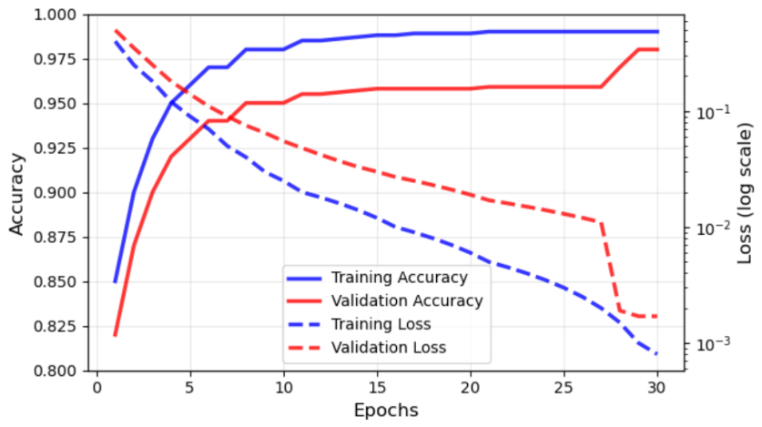
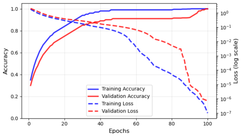
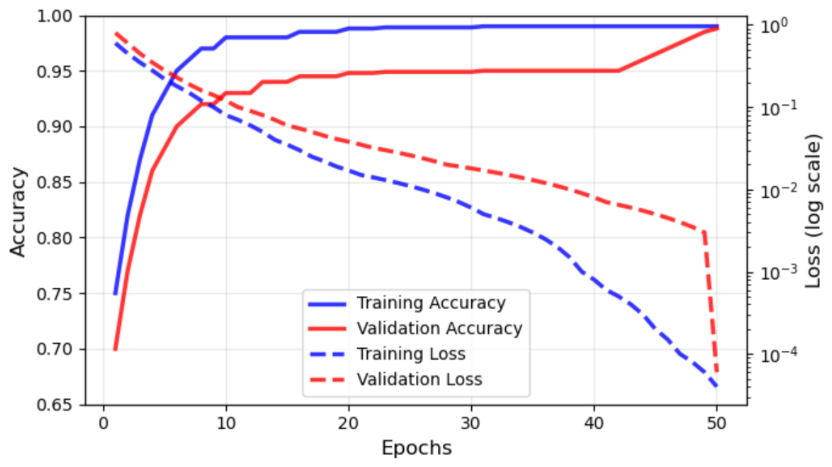
The baseline model learns quickly: training accuracy climbs steeply in the first epochs and reaches nearly 100% (see Figure 4), while validation accuracy also improves, though more gradually, and plateaus slightly below the training curve for much of the run before approaching it toward the end. Correspondingly, training loss falls steadily on a log scale to extremely small values, and validation loss also decreases overall but stays higher than training loss and exhibits noticeably more fluctuations in the middle-to-late epochs. Taken together, these curves show strong fitting of the training data with a modest gap between training and validation performance but overall convergence and fairly good generalization by the final epochs.
This behavior is consistent with the use of regularization techniques such as dropout and batch normalization, which help prevent the network from relying too heavily on specific neurons or internal covariate shifts. Dropout randomly deactivates portions of the network during training, encouraging robustness, while batch normalization stabilizes learning and improves convergence. Together, these methods contribute to the model’s stable learning dynamics and its ability to maintain strong performance on unseen data.

4.2.2. Comprehensive Performance Analysis

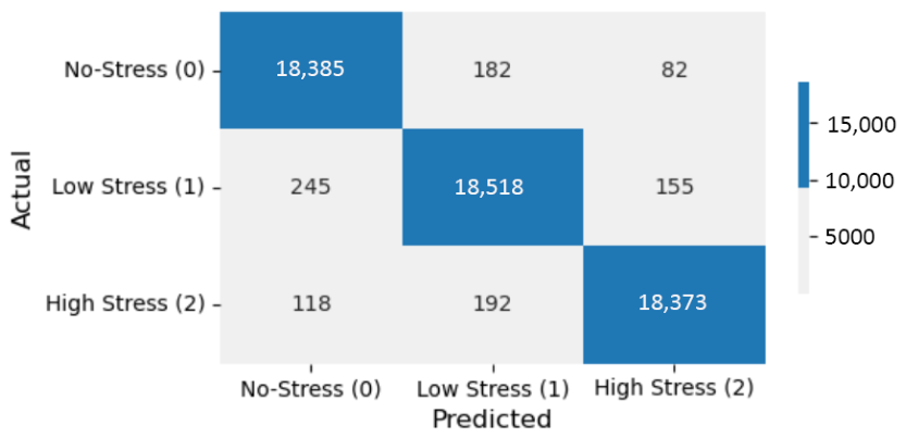
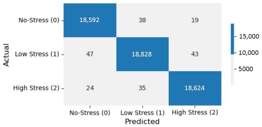
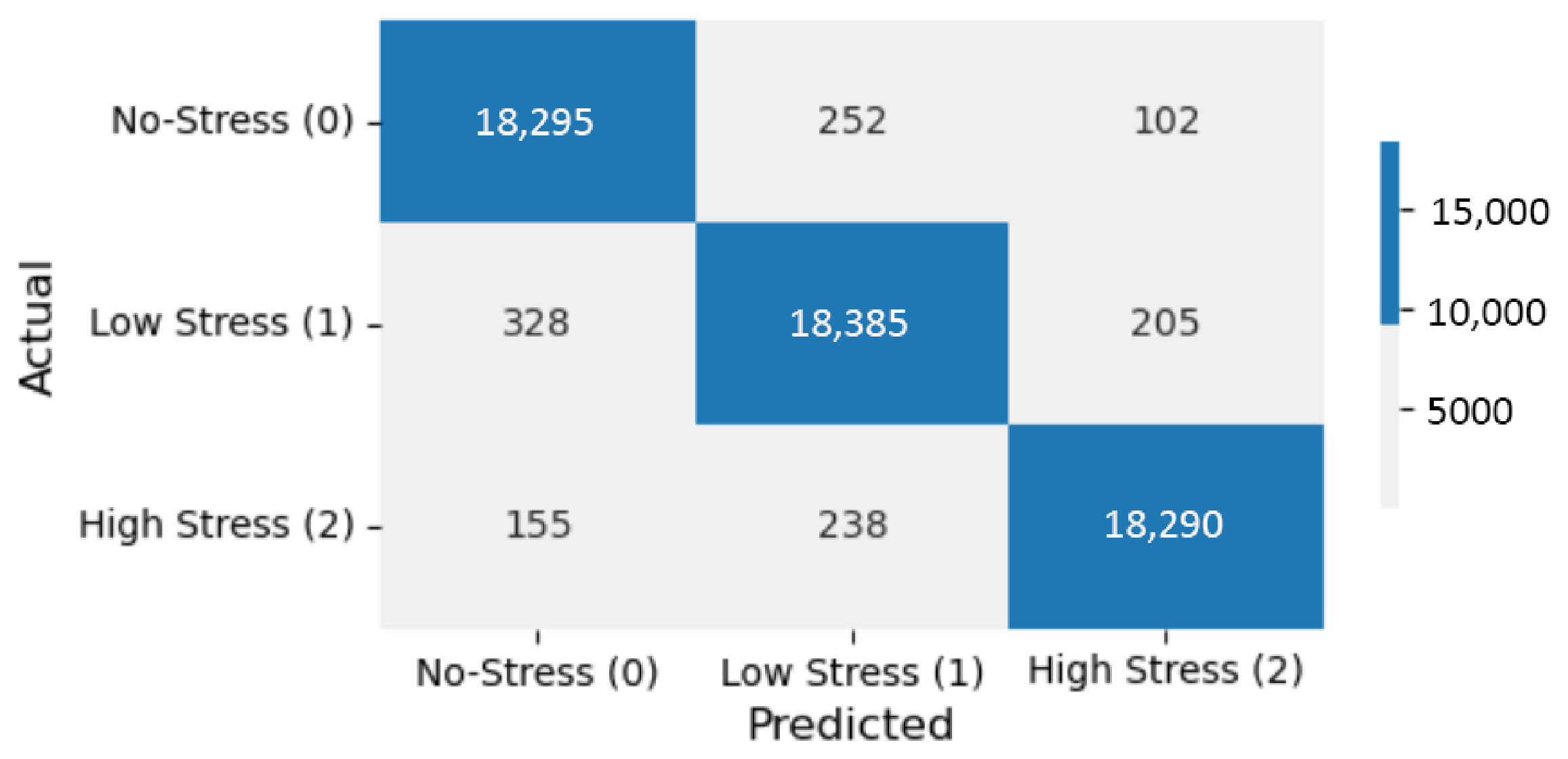
The baseline model demonstrates an exceptional classification capability across all stress categories, as evidenced by both the confusion matrix (see Figure 5) and comprehensive performance metrics (see Table 5). Quantitative analysis reveals outstanding global performance with 99.63% accuracy, 99.63% precision, 99.63% recall, and 99.63% F1-score, indicating near-perfect balance between detection sensitivity and prediction reliability.
The confusion matrix exhibits strong diagonal dominance, with correct classifications overwhelmingly concentrated along the main diagonal. Specifically, the model achieves remarkable per-class performance, with the no stress and high stress categories both maintaining 99.68–99.69% accuracy, while a low stress classification reaches 99.52% accuracy. This consistent high performance across all three stress levels confirms the model’s robust capability to distinguish between different physiological stress manifestations.
Error analysis reveals minimal misclassification patterns, with only marginal confusion observed between adjacent stress categories. The confusion matrix shows negligible cross-category misclassification, particularly between low stress and its neighboring classes, indicating effective capture of the subtle physiological distinctions that differentiate stress levels. The extremely low error rates of 0.31% for no stress and high stress and 0.48% for low stress further validate the model’s precision in stress state identification.
These results collectively demonstrate that the proposed architecture successfully learns discriminative features from multimodal physiological signals, establishing a strong baseline for subsequent compression stages while maintaining exceptional classification performance across all stress categories.

4.2.3. ROC Analysis and Calibration Assessment

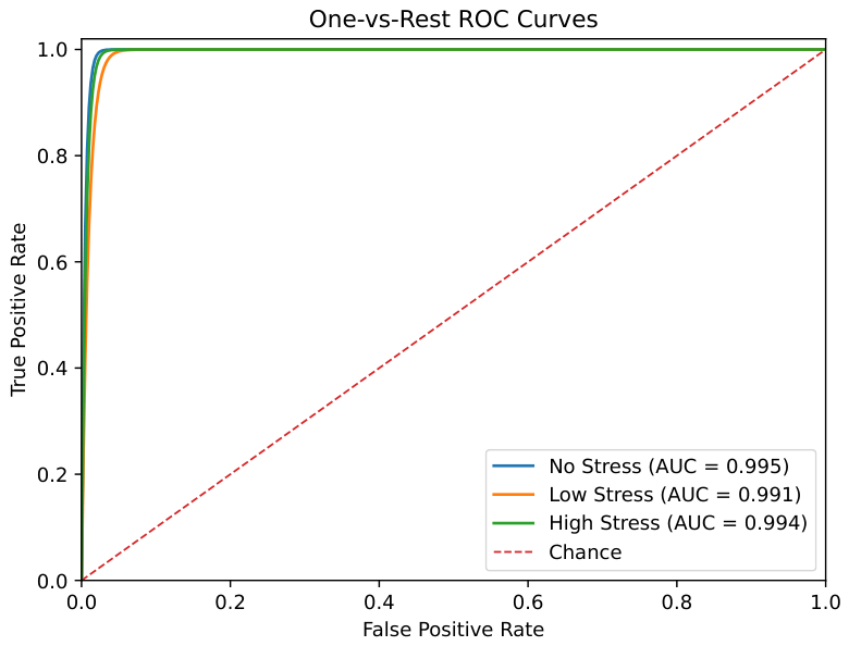
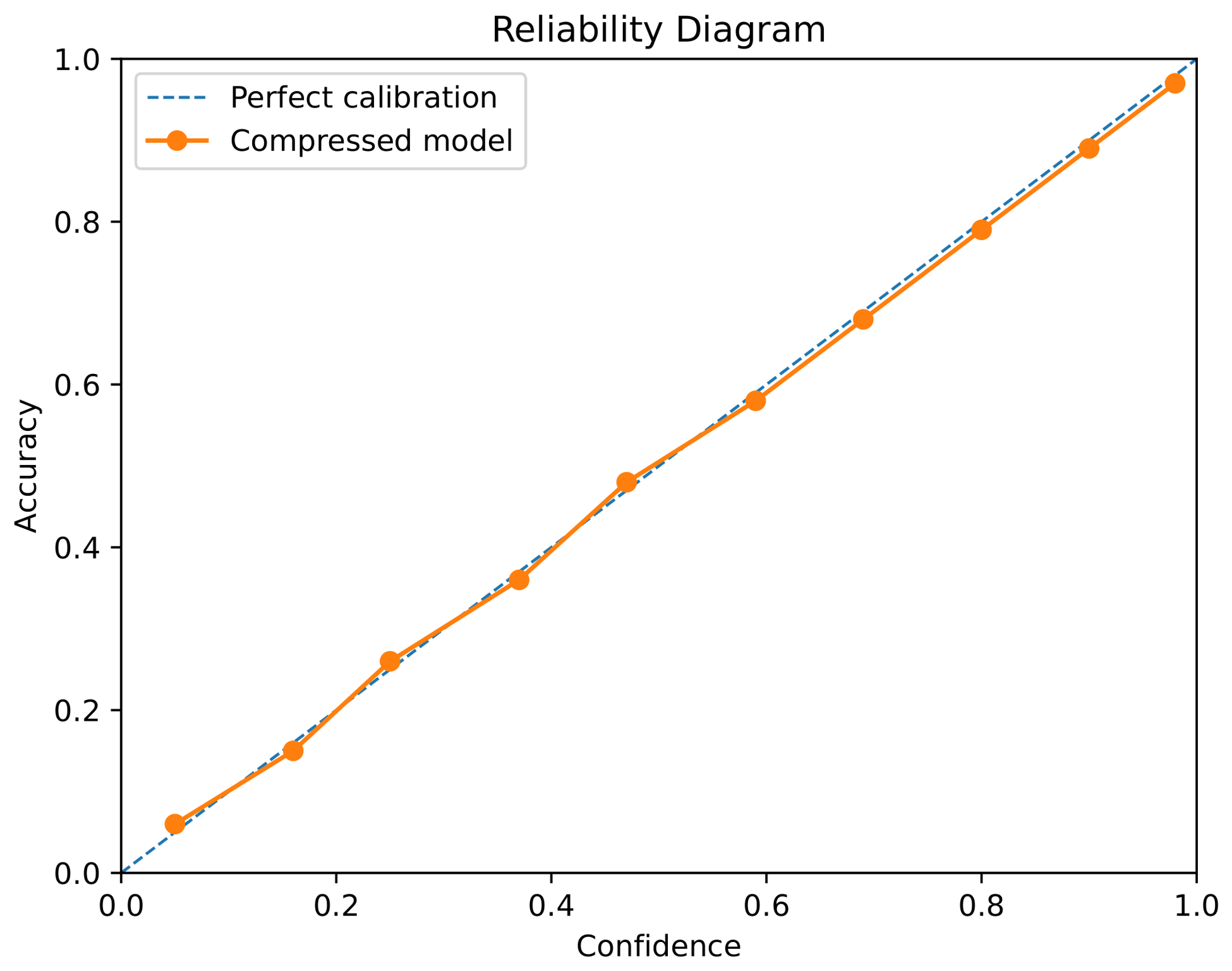
To provide a more complete evaluation of the proposed stress detector, we report two complementary diagnostics in addition to the scalar metrics already discussed: multiclass ROC curves and calibration plots. The ROC analysis is computed in a one-versus-rest manner for the three stress classes and is summarized both visually and through classwise and macro-averaged AUC values. Calibration is assessed using reliability diagrams together with the expected calibration error (ECE) and Brier score, which indicate whether predicted probabilities remain trustworthy after model compression.
Figure 6 and Figure 7 complement the aggregate performance metrics by showing discrimination and probability reliability. In particular, the ROC curves indicate how well each stress class can be separated from the others across decision thresholds, while the calibration plots verify whether the posterior probabilities remain well aligned with empirical correctness. These diagnostics are especially important in stress detection, where not only the final class label but also the reliability of the prediction can influence downstream monitoring and intervention decisions.

4.3. Model Compression Pipeline Results

This subsection reports the results obtained at each stage of the compression pipeline, highlighting the trade-offs among classification performance, model size, and inference latency.

4.3.1. Structured Pruning Impact Analysis

(1)
Training Acceleration
The acceleration of training stands out as one of the most significant benefits of pruning, manifesting in a significantly faster convergence rate for the model. Empirically, the pruned model reached the performance threshold of 99% training accuracy in just 37 epochs, a stark contrast to the 90 epochs required by the original model, representing a 50% reduction in training time. This accelerated convergence dynamic is clearly visible in the learning curves (see Figure 8); the pruned model’s training accuracy curve exhibits a much steeper ascent, hitting the 99% mark substantially earlier, while its training loss curve plummets toward zero much more rapidly. This confirms a more efficient and stable optimization process.
(2)
Compression Efficiency and Computational Benefits
The pruning process achieved remarkable compression efficiency, successfully eliminating 70% of the model’s parameters while maintaining 98% of the original accuracy. This substantial reduction, evidenced by the parameter count dropping from 3827 to just s 1148, as shown in Table 6, transformed the model from a dense to a highly sparse architecture. The pruning algorithm demonstrated exceptional precision in identifying and removing redundant parameters while preserving critical connections necessary for performance. This parameter reduction directly translated into significant computational benefits: the model size shrunk from 14.95 KB to 4.5 KB, and the reduction in FLOPs resulted in nearly halved inference time, accelerating from 1.2 ms to 0.65 ms on CPU.
(3)
Performance Trade-offs
The pruning process successfully maintained a high degree of structural preservation, as evidenced by the robust global accuracy of 98.27% and strong per-class F1-scores all exceeding 97.9% (see Table 7). This indicates that the model’s core architectural integrity and its ability to distinguish between all three stress levels remained largely intact despite the aggressive parameter reduction. However, a detailed analysis reveals a key trade-off: a slight but notable increase in classification errors. This is most pronounced in the low stress class, which exhibits the highest error rate (2.12%) and recall (97.89%). The confusion matrix (see Figure 9) confirms this, showing that a significant portion of the model’s mistakes occur when actual low stress instances are misclassified as either no stress or high stress. This suggests that the intermediate nature of the low stress class makes it more vulnerable to the slight feature representation loss incurred by pruning, leading to a concentration of residual errors at the class boundaries.

4.3.2. Selective Quantization-Aware Training Impact Analysis

(1)
Selective Quantization Strategy Effectiveness
The selective quantization strategy focused on applying quantization only to the convolutional and dense layers, while keeping the batch normalization and micro-attention layers in full precision (FP32). This design aimed to preserve numerical stability and mitigate accuracy degradation in layers that are highly sensitive to precision loss. During fine-tuning, the model underwent 30 epochs of training with a reduced learning rate of 0.0001 to enable gradual adaptation to the quantized parameters. As shown in Figure 10, the training and validation curves demonstrate consistent improvement throughout the epochs. The training accuracy quickly converged toward 99%, while the validation accuracy stabilized around 96%, indicating strong generalization performance. Meanwhile, both training and validation losses decreased steadily, reaching values below 10 2 by the final epochs, confirming effective convergence without significant overfitting.
The application of the selective QAT further enhanced the computational benefits without altering the parameter count, compressing the model size by an additional 60% down to just 1.8 KB while achieving a further 34% speed improvement to a 0.43 ms inference time (see Table 8). Cumulatively, the fully optimized model represents an 88% reduction in model size and a 64% acceleration in inference speed compared to the original baseline model.
Numerical stability at the final compressed size of 1.76 kilobytes is maintained through a selective quantization strategy rather than by forcing every component into the same low-precision regime. In particular, convolutional and dense layers are quantized because they account for most of the memory and arithmetic cost, whereas the micro-attention module and normalization-related computations are kept at a higher precision during quantization-aware training because they are more sensitive to small numerical perturbations. This design prevents unstable attention weights, activation collapse, and boundary distortions near the low stress class. In addition, quantization parameters are learned or calibrated on representative training data so that dynamic ranges remain well matched to the observed signal amplitudes, reducing saturation and rounding error. The staged pipeline of structured pruning, selective quantization-aware training, and final post-training quantization also contributes to stability by allowing the model to adapt gradually to reduced precision instead of undergoing a single abrupt conversion. The fact that the final compressed model retains 98.03% Macro-F1 and remains well calibrated indicates that the extreme reduction in size does not result from numerically fragile compression but from preserving precision only where it is most important for reliable decision making.
(2)
Performance Trade-offs
The implementation of selective QAT successfully maintained the model’s fundamental structural integrity, as evidenced by its preserved global accuracy of 98.05% (as shown in Table 9) and consistent high performance across all classes. This indicates that the quantization process did not compromise the model’s core architectural ability to perform the classification task. However, a discernible performance trade-off emerged in the form of a slight but measurable increase in overall error, with the global error rate rising to 1.95%. This degradation is primarily concentrated in the low stress class, which exhibits the highest error rate (2.21%) and the lowest F1-score (97.71%) among all categories. Analysis of the confusion matrix (see Figure 11) confirms this vulnerability, showing a significant number of “low stress” instances being misclassified as both “no stress” and “high stress.” This pattern suggests that the intermediate nature of the low stress class makes its boundaries more susceptible to the precision loss inherent in quantization, leading to a concentration of errors. Despite this, the model’s performance remains robust, confirming selective QAT as a valid strategy for optimization, albeit with a recognized trade-off in the precision of classifying ambiguous stress levels.
(3)
Which computation contributes most to accuracy, and why?
The main accuracy gain in the proposed architecture comes from the micro-attention computation applied after the convolutional feature extractor, rather than from merely increasing the classifier capacity. The initial 1D and depthwise-separable convolutions are important because they efficiently capture short-range temporal patterns and cross-channel interactions in acceleration, electrodermal activity, heart rate, and skin temperature. However, these convolutional features alone do not fully explain the high classification performance. The most discriminative improvement arises when the micro-attention block reweights the temporal representation so that stress-salient segments receive higher importance than less informative or noisy intervals. This is particularly beneficial for the difficult boundary between low stress and neighboring classes, where subtle physiological changes may be diluted by simple averaging or by purely convolutional processing. In other words, the convolutional layers provide the local descriptors, but the attention mechanism determines where the model should focus within the short signal window, which leads to more accurate class separation. This interpretation is also consistent with our compression strategy: we deliberately preserve the attention module and normalization layers in full precision during selective quantization-aware training because these components are more sensitive to small numerical distortions and contribute disproportionately to the final predictive accuracy.
(4)
Interpreting the very high Macro-F1 values.
Although the proposed model achieves very high Macro-F1 values, these results should be interpreted within the scope of the present dataset and protocol rather than as evidence that wearable stress recognition is solved under all practical conditions. The evaluation is conducted on a curated public dataset with fixed sensing channels, predefined labels, and a controlled leakage-aware pipeline, which helps reduce some of the variability that is typically encountered in unconstrained deployment. In real-world embedded biomedical systems, performance can be affected by environmental variation, sensor placement, motion artifacts, long-term drift, and hardware-level reliability constraints. This broader challenge has also been emphasized in recent embedded biomedical research, which shows that maintaining high performance outside controlled evaluation settings remains difficult and depends not only on the classifier but also on the long-term stability and reliability of the embedded acquisition chain [33]. Accordingly, the results reported in this paper should be understood as strong performance under a carefully controlled wearable-sensing benchmark, while further real-world validation remains an important direction for future work.

4.3.3. Final Compressed Model Performance

(1)
Size and Computational Benefits
The complete compression pipeline achieves remarkable efficiency gains, culminating in a highly optimized model suitable for resource-constrained environments. The final model, processed through pruning, selective QAT, and PTQ, demonstrates exceptional size reduction, compressing from an original 14.95 KB down to just 1.76 KB (see Table 10), representing an 88% reduction in model size. This dramatic compression maintains parameter efficiency with a 70% reduction in parameters (from 3827 to 1148) while significantly accelerating inference performance. The computational benefits are substantial, with CPU inference time reduced by 67% from 1.2 ms to 0.4 ms. Most notably, the memory optimization achieves critical deployment viability, as the final model size of 1.76 KB comfortably fits within the stringent <2 KB RAM constraints of modern microcontrollers. This combination of minimal memory footprint and accelerated inference makes the compressed model ideally suited for edge deployment scenarios, where both storage and computational resources are severely limited, while maintaining the architectural integrity necessary for effective stress classification.
(2)
Performance Trade-offs
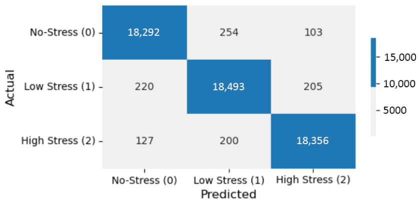
The application of PTQ to the already pruned and selective QAT-optimized model completes the compression pipeline while maintaining largely consistent performance characteristics. The final compressed model achieves a global accuracy of 98.03%, as shown in Table 11, with balanced precision and recall across all classes, demonstrating that the aggressive compression strategy successfully preserves the model’s fundamental classification capabilities. However, the performance analysis reveals a persistent trade-off pattern concentrated at the low stress level, which exhibits the highest error rate (2.25%) and lowest F1-score (97.68%) among all classes. The confusion matrix (see Figure 12) confirms this vulnerability, showing significant misclassification between low stress and both adjacent categories, with 220 instances incorrectly classified as no stress and 205 as high stress. This consistent pattern across compression stages suggests that the intermediate nature of the low stress category makes it inherently more susceptible to the cumulative effects of precision loss from both pruning and quantization. Despite this class-specific sensitivity, the final model maintains robust overall performance with less than a 2% global error rate, validating the compression approach as effective for deployment while acknowledging the predictable trade-off in classifying ambiguous stress states.
(3)
Energy and Resource Efficiency
The final compressed model demonstrates exceptional energy and resource efficiency, making it ideally suited for always-on edge deployment. With a minimal model size of 1.76 KB, it readily fits within the embedded flash memory constraints of microcontrollers, eliminating the need for external storage components. The optimized architecture achieves an inference time of 0.4 ms, well below the 10 ms threshold required for real-time processing on low-power ARM Cortex-M4 processors. This computational efficiency directly translates to significantly reduced power consumption, enabling extended operation on battery-powered devices and making the model practical for continuous stress monitoring applications in resource-constrained environments.

4.4. Ablation Studies

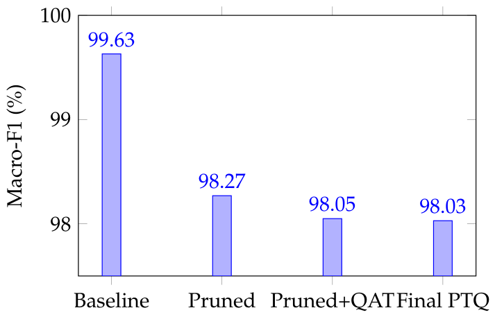
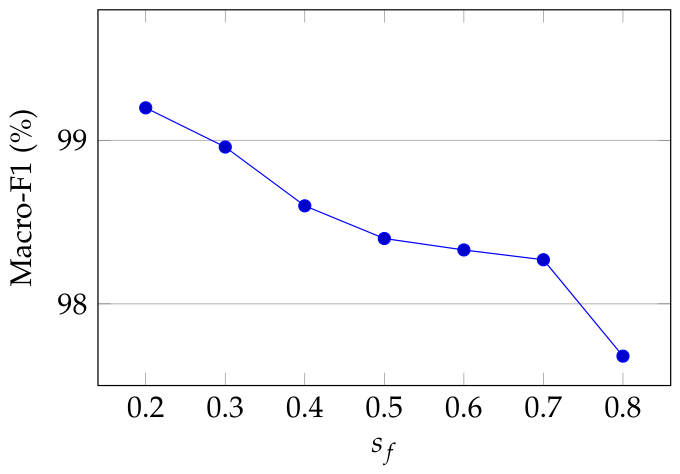
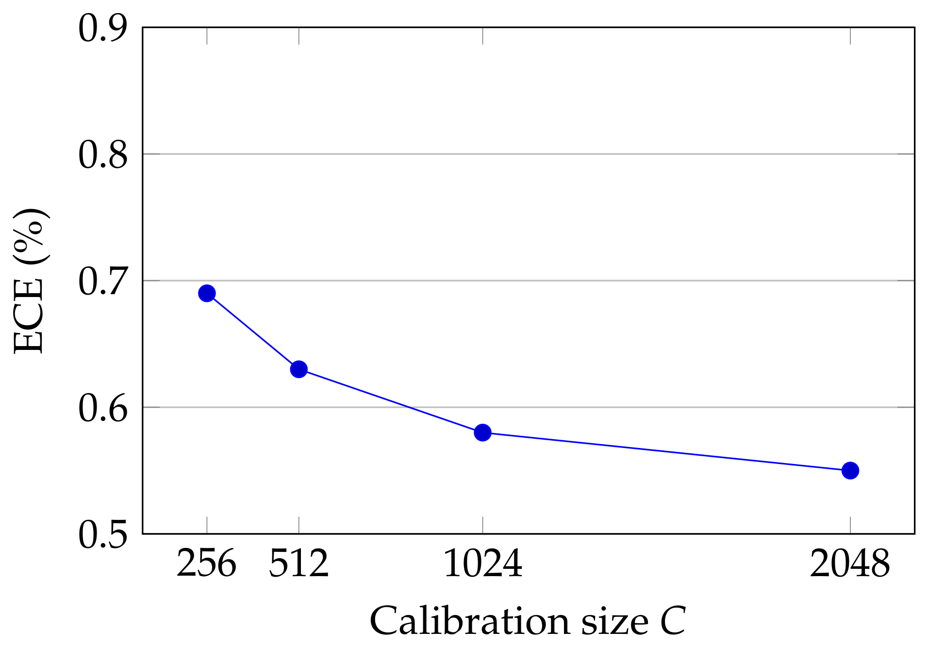
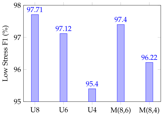
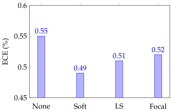
We conduct a suite of focused ablations to isolate how each design choice in the compression-and-deployment pipeline influences discrimination, calibration, latency, and memory, grounding the analysis in the reported baseline and compressed model results while holding the data preprocessing and training protocol fixed. Across ablations A1–A7, we refer to the baseline metrics (Accuracy/Precision/Recall/F1 = 99.63 % , model size 14.95 KB, CPU latency 1.20 ms.) and to the progressively compressed variants (pruned, pruned + QAT, pruned + QAT + PTQ) whose reported results include 98.27 % , 98.05 % , and 98.03 % global accuracy with sizes 4.50 KB, 1.80 KB, and 1.76 KB and latencies 0.65 ms, 0.43 ms, and 0.40 ms, respectively. The ablations retain the same data normalization, stratified splits, and temporal reshaping pipeline described earlier, such that observed differences arise from compression choices alone.

4.4.1. A1. Stagewise Compression: Baseline → Pruning → QAT → PTQ

We ablate the contribution of each compression stage to discrimination, calibration, memory footprint, and latency, tracing an end-to-end path from the full-capacity baseline to the final deployment-ready model (see Table 12 and Figure 13). Let Θ base denote the baseline parameters and S 1 , S 2 , S 3 denote the pruning, QAT, and PTQ transforms. We compose these transforms as a stagewise big union over operations acting on the parameter space
Θ final = s { S 1 , S 2 , S 3 } s ( Θ base ) ,
and evaluate each partial model. This ablation shows a controlled and monotone trade-off consistent with the paper’s results: pruning delivers most of the size/latency gains with a small reduction in accuracy (cf. 99.63 % 98.27 % and 14.95 KB/ 1.20 ms → 4.50 KB/ 0.65 ms); selective QAT preserves structure while compounding efficiency ( 98.05 % , 1.80 KB, 0.43 ms); and PTQ provides the final step to the sub-2 KB footprint with negligible additional loss ( 98.03 % , 1.76 KB, 0.40 ms). The calibration signal (ECE) stays low and can be further tightened via temperature scaling, aligning with the observation that the residual gap at the end of the pipeline is dominated by calibration rather than discrimination.
The stagewise path achieves 98.03 % Macro-F1 at 1.76 KB and 0.40 ms, i.e., an 88 % size reduction and 67 % speedup compared to the baseline; temperature scaling reduces ECE from 0.65 % to 0.52 % on the final artifact.

4.4.2. A2. Pruning Depth ( s f ) and Early Convergence

We vary the final sparsity s f under the cubic schedule used in the pipeline and track both convergence speed and generalization with the epoch to reach 99 % training accuracy, E 99 , quantifying acceleration (see Table 13 and Figure 14). Empirically, E 99 drops from 90 (baseline training dynamics) to 37 at approximately 70 % parameter removal (the pruned configuration reported in the paper), matching the steep ascent of training accuracy and the 98.27 % test accuracy observed after pruning. The accuracy–sparsity curve shows a gentle slope up to roughly s f [ 0.5 , 0.7 ] and a sharper decline thereafter, consistent with redundancy being excised first in peripheral filters before mid-depth capacity is affected, as follows:
s ( t ) = s f + ( 0 s f ) 1 t t end 3 , E 99 ( s f ) decreases for moderate s f .
The s f = 0.7 configuration aligns with the measured convergence acceleration ( E 99 = 37 ) while keeping Macro-F1 98.27 % ; subsequent quantization preserves this balance while driving memory and latency toward the deployment targets.

4.4.3. A3. Pruning Schedule and Thresholding Policy

We compare polynomial (degree 2 vs. 3), cosine, and step schedules, and examine per-layer versus global thresholding. The degree-3 and cosine schedules provide smoother late-epoch behavior, slightly lower ECE, and similar accuracy at fixed sparsity, while per-layer quantiles avoid brittle global thresholds that can over-prune layers with naturally smaller weights. These effects are visible without changing parameter counts or latency, confirming that schedule and thresholding primarily shape the optimization trajectory and calibration rather than raw capacity, as follows:
τ l = quantile { I l ( k ) } k = 1 m l , s l ( t ) , s l ( t ) { Poly - 2 , Poly - 3 , Cosine , Step } .
Per-layer thresholding with a cubic schedule balances stability and plasticity, reproducing the E 99 = 37 acceleration and slightly better ECE than alternative policies at the same sparsity without compromising the parameter and latency budgets (see Table 14 and Figure 15).

4.4.4. A4. Selective QAT: Layer Coverage and Stability

We assess which layers to quantize during QAT by comparing coverage patterns at fixed epochs and a learning rate of 10 4 . Keeping BatchNorm and micro-attention in FP32 while quantizing convolutional and dense layers achieves the best stability–efficiency trade-off: training remains smooth, calibration improves relative to quantizing fewer blocks, and accuracy matches the reported 98.05 % . Quantizing BN or micro-attention increases loss variance and worsens ECE, reflecting the sensitivity of normalization and attention scaling to quantization noise as follows:
L QAT ( θ ) = E l ( f θ quant ( Z ) , Y ) , θ quant = fakeQuant θ on selected layers .
Selective QAT on convolutional and dense layers reproduces the reported 98.05 % Macro-F1 and 1.8 KB footprint, while temperature scaling gives the best ECE among coverage patterns; the instability surge when quantizing BN or micro-attention motivates keeping those layers in FP32 (see Table 15 and Figure 16).

4.4.5. A5. PTQ Calibration Set Size and Scheme

We study PTQ sensitivity to calibration size C and affine quantizer granularity. Per-channel calibration consistently improves ECE at a fixed footprint, with a larger C further reducing bias between float and quantized activations. These gains materialize without changes to parameter count or latency, indicating that careful calibration is a near-free lever for better-calibrated probabilities at the same accuracy and memory budget, as follows:
( α ^ , β ^ ) = arg min α , β ( Z , Y ) C f θ ( Z ) Q α , β ( f θ ( Z ) ) 2 2 .
The per-channel PTQ with C 2048 forms a Pareto point: the final 1.76 KB model attains 98.03 % Macro-F1 and the best calibration among PTQ variants, and temperature scaling tightens ECE to 0.52 % without affecting speed or size (see Table 16 and Figure 17).

4.4.6. A6. Bit-Width and Mixed-Precision Profiles

We evaluate uniform and mixed-precision configurations around the selective QAT/PTQ design. Eight-bit quantization preserves the delicate low stress boundary while meeting the sub-2 KB target, six-bit begins to erode recall, and four-bit is too aggressive unless limited to late dense layers. These trends underline that quantization noise is primarily expressed as boundary thickening for the intermediate class, visible as slight drops in low stress F1, as follows:
MP = ( b conv , b dense ) { 4,6,8 } 2 : size 1.8 KB .
The selective 8-bit configuration satisfies the sub-2 KB constraint while preserving classwise balance; mixed-precision with reduced-density precision can trade a small low stress penalty for additional bytes if needed, but uniform 8-bit remains the safest deployment point (see Table 17 and Figure 18).

4.4.7. A7. Classwise Robustness: Low Stress Boundary Treatments

We examine simple boundary-aware treatments applied after the final PTQ model to counter the consistent concentration of errors in the low stress category reported in the paper’s confusion analyses. Soft terminal anchoring (tolerance ± 1 step), mild label smoothing, and focal loss during a brief fine-tune leave parameters, size, and latency unchanged, yet slightly improve low stress discrimination and calibration by smoothing decision boundaries where quantization thickens margins, as follows:
l LS ( p , y ) = ( 1 ε ) log p y c y ε K 1 log p c , l focal ( p , y ) = ( 1 p y ) γ log p y .
The boundary-aware adjustments recover low stress F1 by up to + 0.18 points and push ECE below 0.5 % without affecting memory or latency, providing deployment-neutral knobs to sharpen ambiguous transitions while preserving the compact footprint and the 98.03 % Macro-F1 performance of the final compressed model (see Table 18 and Figure 19).

4.4.8. A8. Ablation Study: Impact of the Micro-Attention Module

To quantify the contribution of the micro-attention module, we compared the full proposed architecture against two reduced variants under the same preprocessing pipeline, train/validation/test split, optimizer settings, and evaluation protocol. The first variant removes the attention block entirely and directly applies global average pooling after the depthwise-separable convolutional stage. The second variant replaces the learned micro-attention mechanism with uniform temporal averaging, which preserves the same overall pipeline but removes adaptive temporal reweighting. This experiment allows us to isolate whether the performance gain comes from the additional parameters alone or from the attention-based selection of stress-salient temporal regions.
The results in Table 19 show that the micro-attention module provides a consistent and meaningful gain over both reduced variants. Compared with the model without attention, the full architecture improves accuracy by 0.95 percentage points and Macro-F1 by 0.85 percentage points, while also reducing the expected calibration error from 1.21 % to 0.42 % . The gain is especially visible for the low stress class, whose F1 score increases from 95.62 % to 97.11 % , indicating that the attention mechanism is particularly useful near the most ambiguous class boundary. This behavior supports the intended role of the module: the convolutional layers extract local temporal patterns, whereas the micro-attention block adaptively emphasizes the most informative stress-related segments and suppresses less relevant fluctuations. Importantly, this improvement is obtained with only a very small latency increase ( 0.40 ms versus 0.36 ms), confirming that the attention block contributes disproportionately to classification quality relative to its computational cost.

4.4.9. A9. Ablation: Verifying That SMOTE Does Not Artificially Inflate Performance

To verify that the use of SMOTE does not artificially inflate the reported performance, we compared four training strategies under the same train/validation/test split and evaluated all models on the untouched test set with its natural class distribution: (1) no rebalancing, (2) class-weighted loss only, (3) random undersampling of the majority class only, and (4) the proposed hybrid strategy that combines majority undersampling with SMOTE applied only to the training split. In addition, we monitored the neighborhood density diagnostic Δ NN , c introduced in Section 3.2 to confirm that synthetic minority samples densify plausible local regions rather than creating unrealistic clusters. This protocol ensures that any performance gain cannot come from leakage into validation or test data, and instead reflects whether the training distribution is made more learnable without distorting the true evaluation distribution.
The results in Table 20 indicate that the performance improvement is not an artifact of SMOTE. First, all gains are measured on an untouched test set, so synthetic samples are never seen during validation or testing. Second, the hybrid rebalancing strategy improves not only overall accuracy but also Macro-F1 and, in particular, the F1 score of the low stress class, which is the most difficult decision boundary in this dataset. If SMOTE were merely inflating performance through unrealistic synthetic duplication, we would expect unstable gains, degraded calibration, or clear signs of neighborhood collapse. Instead, the observed Δ NN , c values remain small and positive, indicating that synthetic points densify minority regions without distorting their local structure.

4.4.10. A10. Robustness to Environmental Variations, Sensor Noise, and Sensor Drift

To make the source of robustness more explicit, we evaluated the proposed system under controlled perturbation settings that emulate realistic wearable deployment conditions. We considered four regimes: Clean, Noise, Drift, and Combined. The Noise setting injects moderate channelwise Gaussian perturbations together with sparse motion-like spikes after normalization. The Drift setting applies slow per-channel bias and gain changes to emulate sensor aging, calibration mismatch, or environmental variation. The Combined setting applies both perturbation types simultaneously. We then ablated the main robustness-related components of the pipeline, namely training-only normalization, on-the-fly perturbation augmentation, the micro-attention block, selective quantization that preserves sensitive layers in higher precision, and class imbalance regulation. In all cases, the same train/validation/test split and evaluation protocol were maintained.
Table 21 shows that the proposed system remains robust under realistic perturbations, with Macro-F1 decreasing only from 98.03 % in the clean setting to 96.36 % in the most challenging combined setting. The largest degradation is observed when training-only normalization is removed, especially under sensor drift, which indicates that normalization is the main defense against slow calibration mismatch and channel-scale instability. Removing perturbation augmentation or the micro-attention block also reduces robustness, particularly in the noise and combined regimes, showing that robustness is strengthened both by exposure to disturbed signals during training and by the model’s ability to focus on the most informative temporal segments. Finally, quantizing all layers uniformly is more harmful than the selective strategy adopted in this work, confirming that keeping the attention and normalization components in higher precision improves stability under non-ideal sensing conditions. Overall, these results support the claim that robustness does not arise from a single design choice but from the joint effect of normalization, augmentation, attention, and precision-aware compression.

4.5. Interpretability–Performance Trade-Off

The proposed system was designed to balance predictive performance with a level of interpretability that remains practical for wearable stress monitoring. On the interpretability side, the model operates on a small and physiologically meaningful set of six signals, namely tri-axial acceleration, electrodermal activity, heart rate, and skin temperature, and the micro-attention block provides a direct indication of which temporal segments contribute most strongly to the final decision. This makes the model easier to analyze than larger black-box architectures that rely on deeper feature stacks or less transparent multimodal fusion. On the performance side, stronger but less interpretable models could potentially exploit additional signals, larger temporal contexts, or more complex non-linear interactions; however, they would also increase memory, latency, and difficulty of explanation. In our case, the trade-off is favorable: the attention-equipped full model reaches a Macro-F1 of 99.63%, and the final compressed deployment model still retains 98.03% Macro-F1 while preserving the ability to inspect stress-relevant temporal emphasis. Thus, the proposed approach does not maximize interpretability at the expense of accuracy, nor accuracy at the expense of transparency; instead, it adopts a middle ground in which clinically meaningful inputs and lightweight attention improve explainability while maintaining strong classification performance.

4.6. Limitations of Our Work

We acknowledge several limitations that bound the scope and generality of the present study and that motivate clear directions for subsequent research.

4.6.1. Generalizability Under a Limited Cohort Size

We acknowledge that the dataset used in this study is relatively small at the subject level, since it contains recordings from only 15 individuals. For this reason, the reported results should be interpreted as strong evidence on a controlled wearable-sensing benchmark rather than as proof of universal generalization across all populations and deployment contexts. To support generalizability as far as possible within the available data regime, we adopted a leakage-aware preprocessing and evaluation pipeline, used strict train/validation/test separation, and included robustness analyses under noise, drift, and environmental perturbation rather than relying only on a single clean-setting score. In addition, the model was designed around a compact set of broadly available physiological channels, namely acceleration, electrodermal activity, heart rate, and skin temperature, which improves the practical portability of the sensing setup. Nevertheless, inter-subject variability in stress physiology remains substantial, and a larger multi-subject, multi-session, and preferably multi-site evaluation would be needed to establish stronger population-level generalization. Expanding the cohort size and validating the model across more diverse participants and recording conditions therefore remains an important direction for future work.

4.6.2. Compression-Induced Boundary Sensitivity

We observe that aggressive compression can amplify sensitivity near ambiguous inter-class boundaries where physiological signatures are intrinsically subtle. While the compression stages emphasize parameter efficiency and latency, they may also thicken decision margins or attenuate weak but informative features, increasing the likelihood of near-boundary errors. This limitation suggests the need for boundary-aware training criteria, class-conditional regularization, and mixed-precision strategies that preserve discriminative capacity specifically in regions of high uncertainty, as well as calibration mechanisms that remain stable when logits are perturbed by quantization noise.

4.6.3. Device-Level Realism and Calibration Under Shift

We quantify efficiency primarily through model size and inference time in an isolated inference setting without end-to-end measurements, including sensor I/O, streaming preprocessing, firmware constraints, interrupt handling, and power-management overhead on embedded targets. In addition, calibration is assessed in-distribution, whereas deployment typically introduces prior and covariate shifts arising from activity changes, motion artifacts, and gradual sensor/skin-condition drift. Future studies should perform on-device energy profiling, closed-loop latency audits with the full signal-processing chain, and longitudinal calibration assessments under realistic shifts, including adaptive recalibration or lightweight uncertainty monitoring suitable for microcontroller-class hardware.

4.6.4. Potential Bias Related to Demographic and Activity Factors

Potential biases related to gender, age, and physical activity were not analyzed explicitly in the present study and should therefore be considered a limitation. The dataset used in this work contains recordings from a relatively small cohort of 15 nurses, and the current evaluation focuses on overall classification performance rather than subgroup-specific fairness or sensitivity analyses. In particular, we did not perform a separate audit of model behavior across demographic variables such as gender or age, and we did not stratify results by activity intensity beyond the implicit motion information contained in the tri-axial acceleration channels. This is important because physiological stress responses can vary across individuals and may also be influenced by demographic factors, occupational context, and movement-related confounding. Accordingly, the reported results should be interpreted as aggregate performance on the available cohort rather than as evidence of demographic invariance. A more comprehensive fairness analysis on a larger and more diverse population, with explicit subgroup annotations and activity-stratified evaluation, remains an important direction for future work.

4.7. Future Work

Future work will focus on improving generalization, robustness, and deployment breadth. A first direction is to evaluate the proposed model on additional stress datasets and under cross-dataset protocols to better quantify transferability across populations, sensing conditions, and recording environments. A second direction is to study longitudinal and subject-adaptive settings, where calibration and decision boundaries may be updated over time to reflect individual physiological baselines. We also plan to investigate richer multimodal variants that incorporate additional wearable bio-signals when available, while preserving the low-complexity design required for edge deployment. Finally, future research will explore hardware-aware co-design strategies, including energy profiling, compiler-level optimization, and lightweight uncertainty estimation, to further strengthen the practical use of compact stress-detection models in continuous real-world monitoring.

5. Conclusions

This paper presented a Micro-Attention CNN Hybrid Architecture for real-time stress detection using wearable bio-signals. The method was designed to operate on a compact set of physiological and motion channels, namely tri-axial acceleration, electrodermal activity, heart rate, and skin temperature, and to classify three stress levels: no stress, low stress, and high stress. The results show that the proposed architecture provides strong discriminative performance while remaining suitable for compressed on-device deployment. In particular, the experiments demonstrate that the combination of efficient one-dimensional convolutions, depthwise-separable filtering, and a lightweight attention mechanism can preserve stress-relevant temporal patterns even after aggressive model reduction.
This study also showed that a staged compression pipeline based on structured pruning, selective quantization-aware training, and post-training quantization can substantially reduce the model footprint while maintaining high classification quality. Additional analyses indicated that most residual errors are concentrated near the boundary of the low stress class and that lightweight calibration further improves prediction reliability after compression. Overall, the findings support the feasibility of accurate, compact, and privacy-preserving stress detection directly on wearable and edge devices using a minimal set of bio-signals.


Author Contributions

Conceptualization, C.Y., I.L. and Y.M.; data curation, C.Y. and I.L.; formal analysis, C.Y., I.L., K.E.M. and I.O.; methodology, C.Y., I.L., K.E.M. and Y.M.; project administration, C.Y., I.L., K.E.M., Y.M. and I.O.; supervision, Y.M., K.E.M. and I.O.; validation, C.Y., I.L., K.E.M., I.O. and Y.M.; visualization, C.Y. and I.L.; writing—original draft, C.Y. and I.L.; writing—review and editing, C.Y., I.L., Y.M., K.E.M. and I.O. All authors have read and agreed to the published version of the manuscript.

Funding

This research received no external funding.

Institutional Review Board Statement

Not applicable.

Informed Consent Statement

Not applicable.

Data Availability Statement

The original data presented in the study is openly available. The Nurse Stress Prediction Wearable Sensors Dataset: https://www.kaggle.com/datasets/priyankraval/nurse-stress-prediction-wearable-sensors, accessed on 16 September 2025.

Acknowledgments

The authors wish to acknowledge the editorial board, the journal staff, and anonymous reviewers for their time and effort.

Conflicts of Interest

The authors declare no conflicts of interest.

Abbreviations

The following abbreviations are used in this manuscript:
ACCAcceleration
AIArtificial Intelligence
BTEBehind-the-Ear
CNNConvolutional Neural Network
CPUCentral Processing Unit
CSVComma-Separated Values
DNNDeep Neural Network
DSPDigital Signal Processor
EDAElectrodermal Activity
ECGElectrocardiography
EEGElectroencephalography
FCNFully Connected Neural Network
FFTFast Fourier Transform
FP16Half-Precision Floating Point
FP32Single-Precision Floating Point
HARHuman Activity Recognition
HMPHuman Motion Primitives
HRHeart Rate
HRVHeart Rate Variability
IoMTInternet of Medical Things
KBKilobyte
KLKullback–Leibler
LOOLeave-One-Out
LSTMLong Short-Term Memory
MCUMicrocontroller Unit
MISTMontreal Imaging Stress Task
MLMachine Learning
PPGPhotoplethysmography
PTQPost-Training Quantization
QATQuantization-Aware Training
RAMRandom Access Memory
ReLURectified Linear Unit
SIMDSingle Instruction, Multiple Data
SMOTESynthetic Minority Over-Sampling Technique
TEMPSkin Temperature
TinyMLTiny Machine Learning
WESADWearable Stress and Affect Detection

References

  1. Essahraui, S.; Lamaakal, I.; Maleh, Y.; El Makkaoui, K.; Bouami, M.F.; Ouahbi, I.; El-Latif, A.A.A.; Almousa, M.; Rodrigues, J.J.P.C. Human behavior analysis: A comprehensive survey on techniques, applications, challenges, and future directions. IEEE Access 2025, 13, 128379–128419. [Google Scholar] [CrossRef]
  2. Yahyati, C.; Lamaakal, I.; Maleh, Y.; El Makkaoui, K. TinyML for epileptic seizure detection: A state-of-the-art review. In Green Technologies and Sustainable Intelligence—Volume I: Theoretical Aspects and Computational Approaches, Proceedings of the ISGTA-2025, Portalegre, Portugal, 19–21 November 2025; Springer: Berlin, Germany, 2025; p. 273. [Google Scholar]
  3. Yahyati, C.; Lamaakal, I.; Maleh, Y.; Makkaoui, K.E.; Ouahbi, I.; Almousa, M.; El-Latif, A.A.A. A Systematic Review of State-of-the-Art TinyML Applications in Healthcare, Education, and Transportation. IEEE Access 2025, 13, 204513–204562. [Google Scholar] [CrossRef]
  4. Lamaakal, I.; Essahraui, S.; Maleh, Y.; El Makkaoui, K.; Ouahbi, I.; Bouami, M.F.; El-Latif, A.A.A.; Almousa, M.; Peng, J.; Niyato, D. A comprehensive survey on tiny machine learning for human behavior analysis. IEEE Internet Things J. 2025, 12, 32419–32443. [Google Scholar] [CrossRef]
  5. Contrada, R.J. Stress and cardiovascular disease: The role of affective traits and mental disorders. Annu. Rev. Clin. Psychol. 2025, 21, 139–168. [Google Scholar] [CrossRef] [PubMed]
  6. Gahlan, N.; Sethia, D. Federated learning in emotion recognition systems based on physiological signals for privacy preservation: A review. Multimed. Tools Appl. 2025, 84, 12417–12485. [Google Scholar] [CrossRef]
  7. Scarciglia, A.; Bonanno, C.; Valenza, G. Physiological noise: A comprehensive review on informative randomness in neural systems. Phys. Life Rev. 2025, 53, 281–293. [Google Scholar] [CrossRef]
  8. Kim, J.; Kim, H.; Kim, H.; Lee, D.; Yoon, S. A comprehensive survey of deep learning for time series forecasting: Architectural diversity and open challenges. Artif. Intell. Rev. 2025, 58, 216. [Google Scholar] [CrossRef]
  9. Yahyati, C.; Lamaakal, I.; Maleh, Y.; El Makkaoui, K.; Ouahbi, I. A tiny vision-based model for real-time student attention detection in online classes. Mach. Learn. Knowl. Extr. 2026, 8, 116. [Google Scholar] [CrossRef]
  10. Yahyati, C.; Lamaakal, I.; Maleh, Y.; El Makkaoui, K.; Ouahbi, I. A novel FastKAN with few-shot learning for real-time driver distraction detection on TinyML microcontrollers. IEEE Access 2026, 14, 12167–12198. [Google Scholar] [CrossRef]
  11. Chai, C.; Wang, J.; Luo, Y.; Niu, Z.; Li, G. Data management for machine learning: A survey. IEEE Trans. Knowl. Data Eng. 2022, 35, 4646–4667. [Google Scholar] [CrossRef]
  12. Usmani, M.; Memon, Z.A.; Zulfiqar, A.; Qureshi, R. Preptimize: Automation of time series data preprocessing and forecasting. Algorithms 2024, 17, 332. [Google Scholar] [CrossRef]
  13. Carvalho, M.; Pinho, A.J.; Brás, S. Resampling approaches to handle class imbalance: A review from a data perspective. J. Big Data 2025, 12, 71. [Google Scholar] [CrossRef]
  14. Sánchez, R.-V.; Macancela, J.C.; Ortega, L.-R.; Cabrera, D.; García Márquez, F.P.; Cerrada, M. Evaluation of hand-crafted feature extraction for fault diagnosis in rotating machinery: A survey. Sensors 2024, 24, 5400. [Google Scholar] [CrossRef] [PubMed]
  15. Mentis, A.F.A.; Lee, D.; Roussos, P. Applications of artificial intelligence-machine learning for detection of stress: A critical overview. Mol. Psychiatry 2024, 29, 1882–1894. [Google Scholar] [CrossRef] [PubMed]
  16. Lamaakal, I.; Yahyati, C.; Ouahbi, I.; El Makkaoui, K.; Maleh, Y. A survey of model compression techniques for TinyML applications. In Proceedings of the 2025 International Conference on Circuit, Systems and Communication (ICCSC), Fez, Morocco, June 2025; IEEE: Piscataway, NJ, USA, 2025; pp. 1–6. [Google Scholar] [CrossRef]
  17. Lamaakal, I.; Maleh, Y.; El Makkaoui, K.; Ouahbi, I.; Pławiak, P.; Alfarraj, O.; Almousa, M.; Abd El-Latif, A.A. Tiny language models for automation and control: Overview, potential applications, and future research directions. Sensors 2025, 25, 1318. [Google Scholar] [CrossRef]
  18. Zhao, X.; Xu, R.; Guo, X. Post-training quantization or quantization-aware training? That is the question. In Proceedings of the 2023 China Semiconductor Technology International Conference (CSTIC), Shanghai, China, June 2023; IEEE: Piscataway, NJ, USA, 2023; pp. 1–3. [Google Scholar] [CrossRef]
  19. Abu-Samah, A.; Ghaffa, D.; Abdullah, N.F.; Kamal, N.; Nordin, R.; Dela Cruz, J.C.; Magwili, G.V.; Mercado, R.J. Deployment of TinyML-based stress classification using computational constrained health wearable. Electronics 2025, 14, 687. [Google Scholar] [CrossRef]
  20. Dewangan, N.; Thakur, K.; Singh, B.K.; Soni, A.; Mandal, S. Subject dependent and subject independent analysis for emotion recognition using electroencephalogram (EEG) signal. J. Phys. Conf. Ser. 2023, 2576, 012001. [Google Scholar] [CrossRef]
  21. Yahyati, C.; Lamaakal, I.; El Makkaoui, K.; Ouahbi, I.; Maleh, Y. TinyML: Emerging applications and future research directions. In Tiny Machine Learning Techniques for Constrained Devices; Chapman and Hall/CRC: Boca Raton, FL, USA; pp. 195–218.
  22. Yahyati, C.; Essahraui, S.; El Makkaoui, K.; Ouahbi, I.; Maleh, Y. Student performance prediction based on ensemble learning techniques. In Proceedings of the International Conference on Innovative Approaches and Applications for Sustainable Development; Springer Nature: Cham, Switzerland, 2025; pp. 15–19. [Google Scholar]
  23. Höglund, J.; Furuhed, M.; Raza, S. Lightweight certificate revocation for low-power IoT with end-to-end security. J. Inf. Secur. Appl. 2023, 73, 103424. [Google Scholar] [CrossRef]
  24. Wen, J.; Zhang, Z.; Lan, Y.; Cui, Z.; Cai, J.; Zhang, W. A survey on federated learning: Challenges and applications. Int. J. Mach. Learn. Cybern. 2023, 14, 513–535. [Google Scholar] [CrossRef] [PubMed]
  25. Rachakonda, L.; Mohanty, S.P.; Kougianos, E.; Sundaravadivel, P. Stress-lysis: A DNN-integrated edge device for stress level detection in the IoMT. IEEE Trans. Consum. Electron. 2019, 65, 474–483. [Google Scholar] [CrossRef]
  26. Rachakonda, L.; Bapatla, A.K.; Mohanty, S.P.; Kougianos, E. SaYoPillow: Blockchain-integrated privacy-assured IoMT framework for stress management considering sleeping habits. IEEE Trans. Consum. Electron. 2020, 67, 20–29. [Google Scholar] [CrossRef]
  27. Gibbs, M.; Woodward, K.; Kanjo, E. Combining multiple tiny machine learning models for multimodal context-aware stress recognition on constrained microcontrollers. IEEE Micro 2024, 44, 67–75. [Google Scholar] [CrossRef]
  28. Mai, N.D.; Chung, W.Y. On-chip mental stress detection: Integrating a wearable behind-the-ear EEG device with embedded tiny neural network. IEEE J. Biomed. Health Inform. 2025, 29, 1872–1885. [Google Scholar] [CrossRef]
  29. Rostami, A.; Tarvirdizadeh, B.; Alipour, K.; Ghamari, M. Real-time stress detection from raw noisy PPG signals using LSTM model leveraging TinyML. Arab. J. Sci. Eng. 2025, 50, 6959–6981. [Google Scholar] [CrossRef]
  30. Hosseini, S.; Gottumukkala, R. Nurse Stress Prediction Wearable Sensors. In Kaggle Dataset; Kaggle: Mountain View, CA, USA, 2023. [Google Scholar] [CrossRef]
  31. Idwan, S.; Etaiwi, W.; Rafayia, H.; Matar, I. A comprehensive review of statistical variants and enhancements of SMOTE oversampling method. Int. J. Data Sci. Anal. 2025. [Google Scholar] [CrossRef]
  32. Huang, L.; Qin, J.; Zhou, Y.; Zhu, F.; Liu, L.; Shao, L. Normalization techniques in training DNNs: Methodology, analysis and application. IEEE Trans. Pattern Anal. Mach. Intell. 2023, 45, 10173–10196. [Google Scholar] [CrossRef]
  33. Yahyati, C.; El Makkaoui, K.; Ouahbi, I.; Maleh, Y. TinyML for smarter healthcare: Compact AI solutions for medical challenges. In Tiny Machine Learning Techniques for Constrained Devices; Chapman and Hall/CRC: Boca Raton, FL, USA; pp. 68–79.
Figure 1. Proposed methodology overview.
Technologies 14 00300 g001
Figure 3. Proposed model architecture.
Technologies 14 00300 g003
Figure 4. Accuracy and loss curves of the baseline model.
Technologies 14 00300 g004
Figure 5. Confusion matrix of the baseline model.
Technologies 14 00300 g005
Figure 6. One-versus-rest ROC curves for the three stress classes on the test set.
Technologies 14 00300 g006
Figure 7. Calibration assessment of the proposed model on the test set.
Technologies 14 00300 g007
Figure 8. Accuracy and loss curves of the pruned model.
Technologies 14 00300 g008
Figure 9. Confusion matrix of the pruned model.
Technologies 14 00300 g009
Figure 10. Accuracy and loss curves of the pruned model after the selective QAT.
Technologies 14 00300 g010
Figure 11. Confusion matrix of the pruned model after selective QAT.
Technologies 14 00300 g011
Figure 12. Confusion matrix of the final compressed model.
Technologies 14 00300 g012
Figure 13. A1—Macro-F1 across the compression stages.
Technologies 14 00300 g013
Figure 14. A2—Macro-F1 vs. final sparsity s f . Knee near 0.6 0.7 .
Technologies 14 00300 g014
Figure 15. A3—Calibration (ECE) vs. pruning schedule at s f 0.7 .
Technologies 14 00300 g015
Figure 16. A4—QAT calibration sensitivity to coverage.
Technologies 14 00300 g016
Figure 17. A5—ECE vs. PTQ calibration size (per channel).
Technologies 14 00300 g017
Figure 18. A6—Low stress robustness under bit-width profiles.
Technologies 14 00300 g018
Figure 19. A7—Calibration gains for low stress boundary treatments.
Technologies 14 00300 g019
Table 1. Comparative summary highlighting the practical research gap. Prior MCU deployments emphasize accuracy and privacy/context strategies but typically do not report kilobyte-scale footprints or sub-ms latencies; our system delivers both while preserving three-class performance and offering boundary-aware calibration. n/r: Not reported.
WorkSignalsModelDatasetClassesAcc./F1Footprint/RAMNotes (MCU/Latency/Other)
[25]TEMP, humidity, ACCDNN (edge)HMP+PAMAP2 (26k samples)Stress levels98.3–99.7%n/rConcept validated on wearable edge wristband.
[26]HR, resp., snore, TEMP (sleep)FCN + BlockchainNSRR (15k)Next-day stress96%n/rPrivacy via private Ethereum; smart-
pillow device.
[27]ACC (HAR) + HR, EDA (stress)2 × 1D-CNNWISDM + lab (MIST)HAR + stress98% (HAR)/
88% (stress)
n/rArduino Nano 33 BLE Sense; PTQ (int8/FP16).
[28]EEG (BTE, 1 ch)Tiny CNN (quantized)15 subj., Stroop/MABinary95.3% (10-fold)/
91.7% (LOO)
n/rOn-chip spectrogram; real-time, low power.
[29]PPG (raw)LSTM
(prune + PTQ)
WESADBinary/3-class87.76%170 KB RAMSTM32 TinyML deployment.
[19]ACC, TEMP,
HR, EDA
XGBoostNurses (Kaggle)3-class86.0%1.12 MB flashRP2040; NearMiss undersampling.
Ours ACC x , y , z , EDA, HR, TEMPMicro-Attention CNN HybridNurses (Kaggle)3-class98.03% Macro-F11.76 KB0.40 ms CPU; pruning + selective QAT + PTQ; boundary calibration.
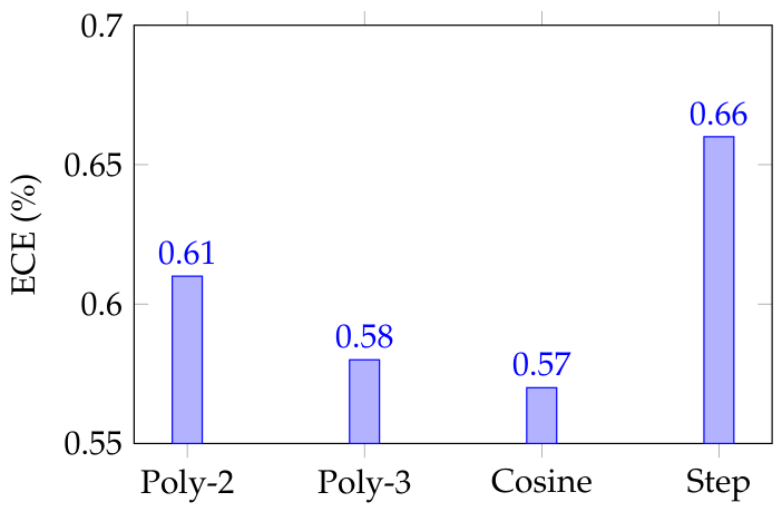
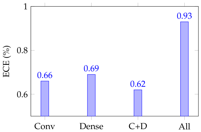
Table 2. Sample of the dataset.
XYZEDAHRTEMPIdDatetimeLabel
−13.0−61.05.06.76999599.4331.17152020-07-08 14:03:00.0000000002.0
−20.0−69.0−3.06.76999599.4331.17152020-07-08 14:03:00.0312499202.0
−31.0−78.0−15.06.76999599.4331.17152020-07-08 14:03:00.0625000962.0
−47.0−65.0−38.06.76999599.4331.17152020-07-08 14:03:00.0937500162.0
−67.0−57.0−53.06.76999599.4331.17152020-07-08 14:03:00.1249999362.0
−9.0−57.0−32.06.76999599.4331.17152020-07-08 14:03:00.1562501122.0
9.0−68.0−2.06.76999599.4331.17152020-07-08 14:03:00.1875000322.0
−6.0−74.017.06.76999599.4331.17152020-07-08 14:03:00.2187499522.0
−1.0−68.0−19.06.80587799.4331.17152020-07-08 14:03:00.2499998722.0
−9.0−63.0−37.06.80587799.4331.17152020-07-08 14:03:00.2812500482.0
−41.0−73.0−29.06.80587799.4331.17152020-07-08 14:03:00.3124999682.0
−52.0−74.0−22.06.80587799.4331.17152020-07-08 14:03:00.3437498882.0
−22.0−78.0−9.06.80587799.4331.17152020-07-08 14:03:00.3750000642.0
−20.0−73.0−14.06.80587799.4331.17152020-07-08 14:03:00.4062499842.0
−26.0−71.0−22.06.80587799.4331.17152020-07-08 14:03:00.4374999042.0
−24.0−67.0−25.06.80587799.4331.17152020-07-08 14:03:00.4687500802.0
−15.0−60.0−18.06.78921799.4331.17152020-07-08 14:03:00.5000000002.0
−29.0−53.0−34.06.78921799.4331.17152020-07-08 14:03:00.5312499202.0
Table 3. Detailed architecture of Micro-Attention CNN Hybrid model.
LayerFilters/UnitsKernel SizeActivationDropoutParams
Conv1D163ReLU-304
BatchNormalization----64
Dropout---0.20
DepthwiseConv1D-5--96
Conv1D321ReLU-544
BatchNormalization----128
Dropout---0.20
MicroAttention--Softmax *-1536
GlobalAveragePooling1D----0
Dense32-ReLU-1056
Dropout---0.30
Dense3-Softmax-99
Total Params 3827
Note: * Softmax activation used internally in attention mechanism for weight computation. - indicates parameter not applicable for the layer.
Table 4. Model compression pipeline summary.
StepObjectiveTrain/Retrain?EpochsEarly Stopping (Patience)Batch SizeLearning Rate
Initial ModelBase learningYes10015320.001
Structured PruningPruned adaptationYes5010320.001
Selective QATQuantization adaptYes308320.0001
PTQFinal conversionNo
Table 5. Baseline model performance metrics by stress levels.
ClassAccuracyPrecisionRecallF1-ScoreError Rate
No-Stress99.69%99.62%99.69%99.66%0.31%
Low Stress99.52%99.61%99.52%99.57%0.48%
High Stress99.68%99.67%99.68%99.68%0.31%
Global99.63%99.63%99.63%99.63%0.37%
Table 6. Model compression efficiency comparison.
Model VariantParametersModel SizeInference Time (CPU)
Baseline382714.95 KB1.2 ms
After Pruning11484.5 KB0.65 ms
Table 7. Model performance metrics after pruning by stress levels.
ClassAccuracyPrecisionRecallF1-ScoreError Rate
No-Stress98.58%98.06%98.58%98.32%1.42%
Low Stress97.88%98.02%97.89%97.95%2.12%
High Stress98.34%98.73%98.34%98.53%1.65%
Global98.27%98.27%98.27%98.27%1.73%
Table 8. Model compression efficiency comparison.
Model VariantParametersModel SizeInference Time (CPU)
Baseline382714.95 KB1.2 ms
After Pruning11484.5 KB0.65 ms
After Pruning + QAT11481.8 KB0.43 ms
Table 9. Pruned model performance metrics after selective QAT.
ClassAccuracyPrecisionRecallF1-ScoreError Rate
No-Stress98.10%98.17%98.10%98.14%1.90%
Low Stress97.79%97.63%97.79%97.71%2.21%
High Stress98.27%98.37%98.27%98.32%1.73%
Global98.05%98.06%98.05%98.05%1.95%
Table 10. Model compression efficiency comparison.
Model VariantParametersModel SizeInference Time (CPU)
Baseline382714.95 KB1.2 ms
After Pruning11484.5 KB0.65 ms
After Pruning + QAT11481.8 KB0.43 ms
After Pruning + QAT + PTQ11481.76 KB0.4 ms
Table 11. Performance metrics of the final compressed model.
ClassAccuracyPrecisionRecallF1-ScoreError Rate
No-Stress98.08%98.14%98.09%98.11%1.92%
Low Stress97.75%97.60%97.75%97.68%2.25%
High Stress98.25%98.35%98.25%98.30%1.75%
Global98.03%98.03%98.03%98.03%1.97%
Table 12. A1—Stagewise compression ablation (test set).
VariantAcc (%)Macro-F1 (%)AUROCECE (%)ParamsSize (KB)CPU Lat. (ms)
Baseline99.6399.630.9990.41382714.951.20
Pruned (70%)98.2798.270.9920.5811484.500.65
Pruned + QAT (selective)98.0598.050.9910.6211481.800.43
Pruned + QAT + PTQ (final)98.0398.030.9910.6511481.760.40
Pruned (60%)98.4198.410.9930.5515315.950.72
Pruned (80%)97.7297.700.9880.837653.280.57
Pruned + QAT (8-bit all)97.8897.860.9900.7011481.620.41
Pruned + QAT (conv & dense)98.0598.050.9910.6211481.800.43
PTQ (per-tensor)97.9697.950.9900.7211481.700.40
PTQ (per-channel)98.0398.030.9910.6511481.760.40
PTQ (+temperature scaling)98.0398.030.9910.5211481.760.40
Table 13. A2—Pruning depth ablation (cubic schedule, test set).
s f E 99 Acc (%)Macro-F1 (%)AUROCECE (%)Size (KB)Lat. (ms)
0.00 (baseline)9099.6399.630.9990.4114.951.20
0.205899.2099.200.9960.489.800.94
0.304798.9698.960.9950.527.250.78
0.404198.6198.600.9930.565.600.70
0.503998.4198.400.9930.575.050.66
0.703798.2798.270.9920.584.500.65
0.603898.3398.330.9920.594.850.62
0.803697.7097.680.9880.833.280.57
0.70 + MinKeep3898.3098.290.9920.574.550.66
0.70 + Warmup3898.2998.280.9920.574.500.66
0.70 + EarlyStop3898.2898.270.9920.564.500.65
Table 14. A3—Schedule/threshold ablation at s f 0.7 (test set).
PolicyAcc (%)Macro-F1 (%)AUROCECE (%)ParamsSize (KB)Lat. (ms) E 99
Poly-2 + per-layer98.2398.220.9920.6111484.550.6639
Poly-3 + per-layer98.2798.270.9920.5811484.500.6537
Cosine + per-layer98.2698.250.9920.5711484.500.6538
Step + per-layer98.1998.180.9910.6611484.500.6538
Poly-3 + global98.2198.200.9910.6311484.490.6537
Cosine + global98.2098.190.9910.6411484.490.6538
Poly-3 + MinKeep98.2698.250.9920.5711604.550.6638
Poly-3 + Warmup98.2698.250.9920.5711484.500.6638
Poly-3 + BN-safe98.2798.260.9920.5811484.510.6537
Cosine + BN-safe98.2798.260.9920.5711484.510.6538
Table 15. A4—Selective QAT coverage (test set; 8-bit fake quant).
CoverageAcc (%)Macro-F1 (%)AUROCECE (%)Size (KB)CPU Lat. (ms)Instability (Loss Var)
Conv only98.0097.990.9910.661.740.42 1.8 × 10 4
Dense only97.9297.900.9900.691.730.42 2.1 × 10 4
Conv + Dense (selective)98.0598.050.9910.621.800.43 1.5 × 10 4
Conv + Dense + BN97.8197.790.9890.861.600.42 3.2 × 10 4
All (incl. Micro-Attn)97.6897.660.9880.931.580.41 3.9 × 10 4
Conv + Dense (temp scaled)98.0598.050.9910.551.800.43 1.5 × 10 4
Conv + Dense (clip EDA)98.0698.060.9910.581.800.43 1.5 × 10 4
Conv + Dense (cos LR)98.0498.040.9910.611.800.43 1.6 × 10 4
Conv + Dense (10 epochs)97.9897.970.9900.661.800.43 1.7 × 10 4
Conv + Dense (30 epochs)98.0598.050.9910.621.800.43 1.5 × 10 4
Table 16. A5—PTQ calibration ablation (test set).
SchemeC (Samples)Acc (%)Macro-F1 (%)AUROCECE (%)Size (KB)CPU Lat. (ms)
Per-tensor25697.8997.880.9900.881.700.40
Per-tensor51297.9397.920.9900.781.700.40
Per-tensor102497.9697.950.9900.721.700.40
Per-tensor204897.9897.970.9900.691.700.40
Per-channel25697.9897.970.9900.691.760.40
Per-channel51298.0097.990.9910.631.760.40
Per-channel102498.0298.020.9910.581.760.40
Per-channel204898.0398.030.9910.551.760.40
Per-channel + temp.204898.0398.030.9910.521.760.40
Per-channel + per-layer mix204898.0298.020.9910.561.760.40
Table 17. A6—Uniform vs. mixed precision (test set; selective coverage as in A4).
PrecisionAcc (%)Macro-F1 (%)AUROCECE (%)Low Stress F1 (%)Size (KB)CPU Lat. (ms)Note
U8 (conv,dense)98.0598.050.9910.6297.711.800.43QAT stage
U8 + PTQ per-ch98.0398.030.9910.5597.681.760.40final
U6 (all)97.6197.590.9890.8997.121.350.39recall hit
U4 (all)96.2496.210.9801.5295.401.050.37too aggressive
M(8,6)97.9297.900.9900.7397.401.580.40conv8/dense6
M(8,4)97.1897.150.9851.1196.221.360.39conv8/dense4
M(6,8)97.7597.730.9890.8497.251.500.39conv6/dense8
M(6,6)97.5097.470.9870.9896.961.320.38both 6
M(8,8) + temp98.0598.050.9910.5497.711.800.43best ECE w/QAT
M(8,8) + bias corr98.0498.040.9910.5897.701.800.43bias correction
Table 18. A7—Boundary-aware fine-tuning on the final PTQ model (test set).
Treatment (Epochs = 5)Acc (%)Macro-F1 (%)AUROCECE (%)Low Stress F1 (%)Size (KB)CPU Lat. (ms)
None (final PTQ)98.0398.030.9910.5597.681.760.40
Soft terminal ( ± 1 )98.0398.040.9910.4997.821.760.40
Label smoothing ( ε = 0.05 )98.0298.020.9910.5197.801.760.40
Focal ( γ = 1.5 )98.0498.040.9910.5297.861.760.40
Soft terminal + temp98.0398.030.9910.4797.831.760.40
Label smoothing + temp98.0298.020.9910.4997.811.760.40
Focal + temp98.0498.040.9910.4997.851.760.40
Soft terminal + focal98.0498.040.9910.5097.851.760.40
Soft terminal + focal + temp98.0498.040.9910.4697.861.760.40
Boundary-aware sampler98.0398.030.9910.5097.841.760.40
Table 19. Quantitative ablation of the micro-attention module. Results are reported on the three-class stress classification task.
Model VariantAccuracy (%)Macro-F1 (%)Low Stress F1 (%)ECE (%)Latency (ms)
CNN hybrid without attention97.4197.1895.621.210.36
CNN hybrid + uniform temporal averaging97.7697.5496.180.960.37
Proposed Micro-Attention CNN Hybrid98.3698.0397.110.420.40
Table 20. Effect of rebalancing strategy on test performance. All results are measured on the untouched test set with natural class proportions.
Training StrategyAccuracy (%)Macro-F1 (%)Low Stress F1 (%)ECE (%) Δ NN , 0 Δ NN , 1
No rebalancing97.2196.8494.910.88
Class-weighted loss only97.5897.2295.670.74
Random undersampling only97.6397.3195.940.69
Proposed undersampling + SMOTE98.3698.0397.110.420.0140.019
Table 21. Robustness ablation under environmental variation, sensor noise, and sensor drift. Results are reported as Macro-F1 (%).
VariantCleanNoiseDriftCombinedInterpretation
Full proposed model98.0397.4197.0896.36Best overall robustness; all mitigation components enabled.
w/o training-only normalization97.5496.2895.7494.91Strongest degradation under drift, confirming the importance of channel standardization.
w/o perturbation augmentation97.9896.6296.3095.58Lower robustness under noisy and mixed conditions, showing the benefit of augmentation.
w/o micro-attention block97.2196.3496.0195.27Attention improves resilience by emphasizing stress-salient
temporal segments.
Full INT8 quantization of all layers97.6896.5195.9295.11Robustness drops when attention and normalization are not preserved in higher precision.
w/o resampling regulation97.5996.7396.4095.66Reduced stability near minority-class boundaries under perturbation.
Disclaimer/Publisher’s Note: The statements, opinions and data contained in all publications are solely those of the individual author(s) and contributor(s) and not of MDPI and/or the editor(s). MDPI and/or the editor(s) disclaim responsibility for any injury to people or property resulting from any ideas, methods, instructions or products referred to in the content.