AIoT Ecosystem for Intelligent Water Quality Monitoring Through Edge Processing and Generative Artificial Intelligence

Abstract

Water quality monitoring remains a critical challenge for achieving Sustainable Development Goal 6, particularly in rural and resource-constrained environments where conventional laboratory-based methods are costly and slow. This study presents the development and field validation of an Artificial Intelligence of Things (AIoT) ecosystem for intelligent, low-cost, and real-time water quality assessment using edge computing and generative artificial intelligence. The system integrates a laboratory-developed multiparameter probe measuring temperature, pH, dissolved oxygen, and electrical conductivity with a mobile application and a cloud-based backend. Field validation was conducted in riverine environments in the municipality of Pueblo Bello (Cesar, Colombia), where the system was deployed for in situ data acquisition and real-time inference. A supervised Artificial Neural Network (ANN) was trained to classify water quality based on a Water Quality Index (WQI) ground truth derived from a public dataset, employing KNN-based missing data imputation, interquartile range outlier filtering, stratified balancing, and grid search hyperparameter optimization. The best-performing model achieved 85.1% accuracy and an AUC of 0.87 using only four physical parameters and was successfully deployed in TensorFlow Lite format on both the embedded probe and the mobile application with sub-millisecond inference time. Integration with a generative AI backend provides contextual natural-language interpretations of measurements. These results demonstrate that reduced-parameter edge AI systems can provide reliable environmental diagnostics while enhancing accessibility and citizen engagement for participatory water monitoring.

1. Introduction

The United Nations 2030 Agenda for Sustainable Development places water management at the core of global progress through Sustainable Development Goal 6 (SDG 6). This goal not only seeks to guarantee universal access to safe drinking water but also requires improving water quality by reducing pollution and substantially increasing global monitoring efforts [1]. However, achieving these targets faces significant challenges: accelerated industrial growth, uncontrolled urbanization, and the climate crisis have intensified the degradation of water bodies, making water surveillance one of the critical challenges of this century [2].

In recent years, several efforts have focused on developing low-cost monitoring devices to increase accessibility to environmental sensing technologies in resource-constrained contexts. In Colombia, previous research has explored the design of portable multiparametric probes capable of measuring key physicochemical variables such as temperature, pH, electrical conductivity, and dissolved solids using low-cost electronic components [2]. These prototypes demonstrated reliable performance when compared with commercial probes and were specifically designed for deployment in rural communities and remote regions with limited access to conventional laboratory infrastructure. Such developments highlight the feasibility of community-based monitoring systems supported by affordable sensing technologies and mobile data acquisition platforms. Building upon these previous efforts, the present study advances this technological line by integrating edge artificial intelligence, cloud connectivity, and generative AI capabilities into a comprehensive AIoT ecosystem for intelligent environmental diagnostics.

Despite the urgency emphasized by international organizations, conventional monitoring remains anchored in traditional methodologies. Dependence on manual sampling and laboratory analysis, although precise, is logistically unfeasible for dynamic and large-scale surveillance due to high costs and prolonged response times. Over the past decade, the Internet of Things (IoT) has emerged as a disruptive technology to mitigate this gap by enabling remote environmental data acquisition. Nevertheless, traditional IoT systems face an operational bottleneck: total dependence on cloud connectivity. In rural or geographically remote contexts, where network infrastructure is deficient, this centralization produces unacceptable latency and critical service failures [3]. Furthermore, these systems typically store raw data, delivering isolated numerical values (pH, dissolved oxygen, conductivity) that lack immediate meaning for citizens without specialized technical training.

Recent developments in environmental monitoring increasingly rely on Internet of Things (IoT) technologies combined with low-cost sensing devices to improve the spatial and temporal coverage of environmental observations. IoT-based monitoring systems allow the distributed measurement of physicochemical parameters such as temperature, pH, turbidity, and electrical conductivity through embedded sensor nodes connected via wireless communication networks. These systems support real-time monitoring and enable automated environmental analysis using data-driven approaches, including machine learning techniques such as artificial neural networks and K-Nearest Neighbors for water quality classification and anomaly detection [4].

In addition, in recent reviews also highlight the growing use of low-cost IoT platforms based on microcontrollers such as ESP32 and Arduino [5]. These platforms enable scalable deployments in rural and resource-constrained environments by integrating wireless communication technologies such as Wi-Fi and LoRa to transmit environmental data to cloud platforms for storage, visualization, and analysis.

Despite these advances, most existing systems still depend primarily on centralized cloud processing. This architecture can limit the ability to perform real-time inference directly at the sensing node, particularly in remote locations where connectivity may be intermittent or unreliable. Consequently, the integration of edge artificial intelligence into low-cost IoT sensing architecture has emerged as an important research direction to improve system autonomy and responsiveness in environmental monitoring applications.

At the same time, although IoT technologies have significantly improved the collection of environmental data, many studies continue to focus mainly on hardware design, sensor deployment, and communication protocols. For instance, low-cost IoT-enabled agrometeorological stations have demonstrated considerable potential for climate-smart agriculture by enabling continuous monitoring of environmental variables such as temperature, humidity, rainfall, and soil moisture.

Similarly, the development of low-cost soil moisture sensing systems has facilitated real-time irrigation scheduling and improved water-use efficiency in agricultural systems [6]. However, despite their technical performance, the information generated by these systems is often presented as raw measurements or technical indicators that require specialized knowledge to interpret. This limits their accessibility for farmers, citizens, and other local stakeholders.

In recent years, artificial intelligence techniques have also been increasingly integrated into environmental monitoring systems to enhance predictive capabilities in applications such as hydrological forecasting, water quality monitoring, and irrigation management [7]. Nevertheless, many AI-based models operate as black-box systems, where the reasoning behind predictions is not easily interpretable by practitioners or community users.

As a result, environmental monitoring systems often face the well-known challenge of being “data rich but information poor”, where large volumes of data are collected but not effectively transformed into actionable knowledge for decision-making [8]. Therefore, an important research challenge lies in developing environmental monitoring systems that not only acquire and process environmental data but also translate complex datasets into interpretable and actionable information for non-expert users, including citizens, farmers, and local decision-makers.

To address this gap, this study proposes an AIoT-based environmental monitoring framework that integrates low-cost sensing devices with edge artificial intelligence and interpretable data visualization mechanisms. The proposed system aims to improve not only environmental data acquisition, but also the accessibility and interpretability of environmental information to support community-level decision-making. By integrating deep learning algorithms directly into sensor hardware or mobile devices, intelligence can be decentralized, enabling local inference and immediate diagnosis without requiring Internet access [9,10]. A central challenge addressed in this proposal is dimensional restriction: the system infers water status using only the four physical parameters measurable by the available probe (Temperature, pH, Dissolved Oxygen, and Electrical Conductivity).

Although the standard Water Quality Index (WQI) requires biological and chemical variables difficult to obtain in field conditions, this research is grounded in the ability of neural networks to classify water quality based on these four key variables, which act as important indicators of chemical stability and biological activity within aquatic ecosystems [10]. This capability is fundamental for early contaminant detection using low-cost hardware at sampling sites.

Simultaneously, advances in Generative Artificial Intelligence and Large Language Models (LLMs) open opportunities for democratizing water science [11]. While the ANN classifier provides a binary response (contaminated/not contaminated), integration with a generative backend contextualizes physicochemical data, translating them into natural-language reports that explain ecological implications and suggest preventive actions [6]. When integrated with citizen science strategies—where users georeference and share collected samples in collaborative networks—this approach has the potential to create more resilient and transparent environmental monitoring systems aligned with SDG 6 governance goals [12].

This article presents the development and validation of a comprehensive AIoT ecosystem for intelligent water quality monitoring. The main contributions of this work are:

Reduced-Parameter Inference: Implementation of an optimized binary classification neural network using TensorFlow Lite, utilizing only four physical variables, integrated into both a mobile application and a laboratory-developed multiparameter probe for field operation.

Methodological Data Robustness: A data engineering workflow employing multivariate KNN imputation and stratified balancing.

Semantic Interpretability through Generative AI: A cloud-based architecture connected to generative AI that transforms data vectors into descriptive, comprehensible analyses, reducing the knowledge gap for non-expert users.

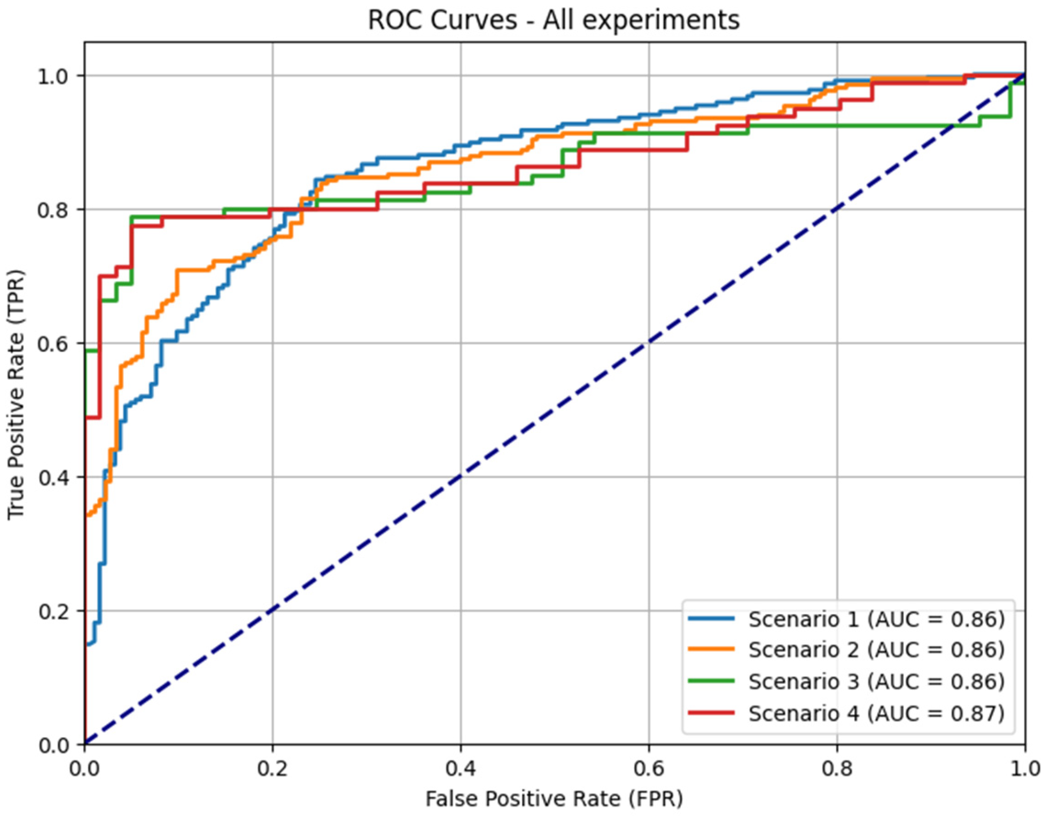
Through evaluation of four experimental scenarios, this study demonstrates how architectural optimization combined with feature enrichment achieves an AUC of 0.87. The results validate the feasibility of using low-cost devices for complex environmental diagnostics, offering a scalable tool for participatory water monitoring.

2. Materials and Methods

This section details the technical components and methodologies that constitute the proposed AIoT ecosystem. The methodological design is based on the integration of a multiparameter probe, developed in a previous project, which serves as the mechanism for real-time data acquisition. Building upon this foundation, the present work develops a software architecture oriented toward edge computing and establishes a workflow for the preprocessing and analysis of environmental information. The following subsections describe the core pillars supporting the system’s operation, ranging from the hardware infrastructure employed to advanced data engineering strategies.

2.1. AIoT Ecosystem Architecture

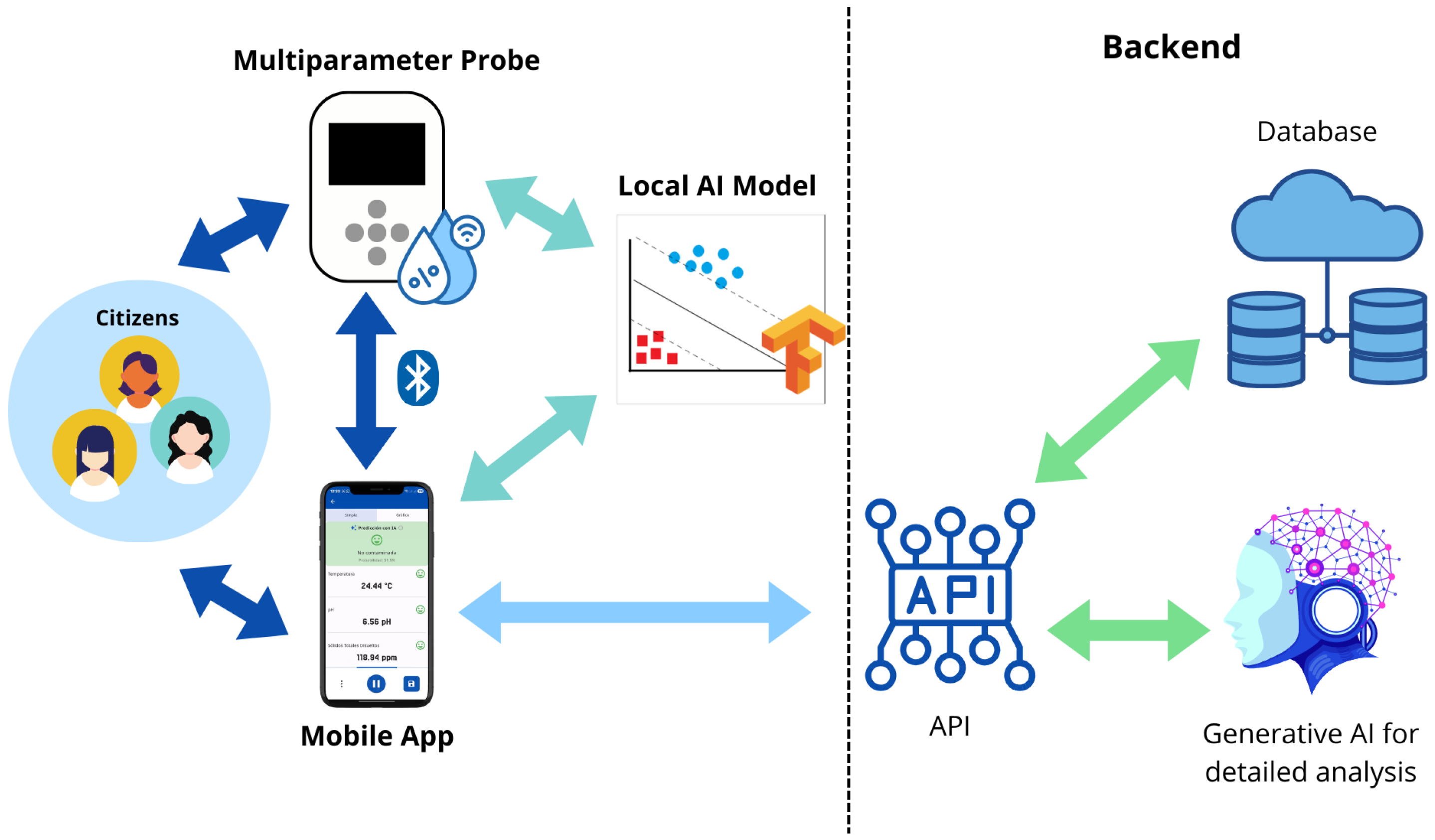
The architecture of the developed system, illustrated in Figure 1, integrates hardware and software components designed to operate in a coordinated manner. The core of data acquisition is a laboratory-developed multiparameter probe, created in a previous project aimed at communities near the city of Valledupar, Colombia [2,13]. This device measures physical variables, using the temperature sensor (model DS18B20, DFRobot, Shanghai, China), the pH sensor (model PH4502C, Generic OEM, China), the dissolved oxygen sensor (model SEN0237-A, DFRobot, Shanghai, China), and the electrical conductivity sensor (model SEN0244, DFRobot, Shanghai, China), and communicates with the mobile application, named Water Probe Hub, via the Bluetooth Low Energy (BLE) protocol.

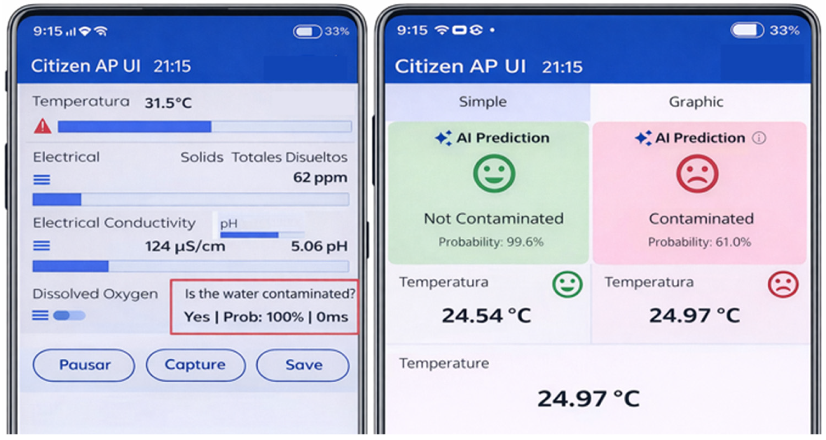
A key element of this architecture is the deployment of the artificial intelligence model both within the probe firmware and in the mobile application. The artificial intelligence model was deployed using TensorFlow Lite (version 2.14.0, Google LLC, Mountain View, CA, USA). The mobile application was developed using TensorFlow for Flutter (version 0.10.4, Google LLC, Mountain View, CA, USA), which provides binding to TensorFlow Lite. This Edge AI configuration enables real-time local inference regarding water status (Contaminated/Not Contaminated) without requiring Internet connectivity.

For advanced processing and data persistence, the system connects to a cloud-based backend. The backend service was implemented using FastAPI (version 0.115.12, FastAPI, USA), exposing a RESTful API that centralizes user management and stores georeferenced samples in a SQL database. Additionally, the API manages communication with a Generative AI service, a generative artificial intelligence service (OpenRouter API, OpenRouter Inc., New York, NY, USA), which receives the physicochemical parameters of each sample and produces interpretative analyses in natural language, providing users with a more detailed and contextualized understanding of water quality beyond simple raw data visualization and binary classification.

2.2. Data Strategy and Preprocessing

The effectiveness of any deep learning model intrinsically depends on the quality and consistency of the training data. In the context of water quality monitoring, records often present specific challenges such as measurement noise, missing values due to sensor failures, and imbalanced sample distributions. To mitigate these issues, a structured preprocessing strategy was implemented in three phases: data refinement through multivariate imputation, outlier detection and removal, and feature engineering for the generation of enhanced supervised labels.

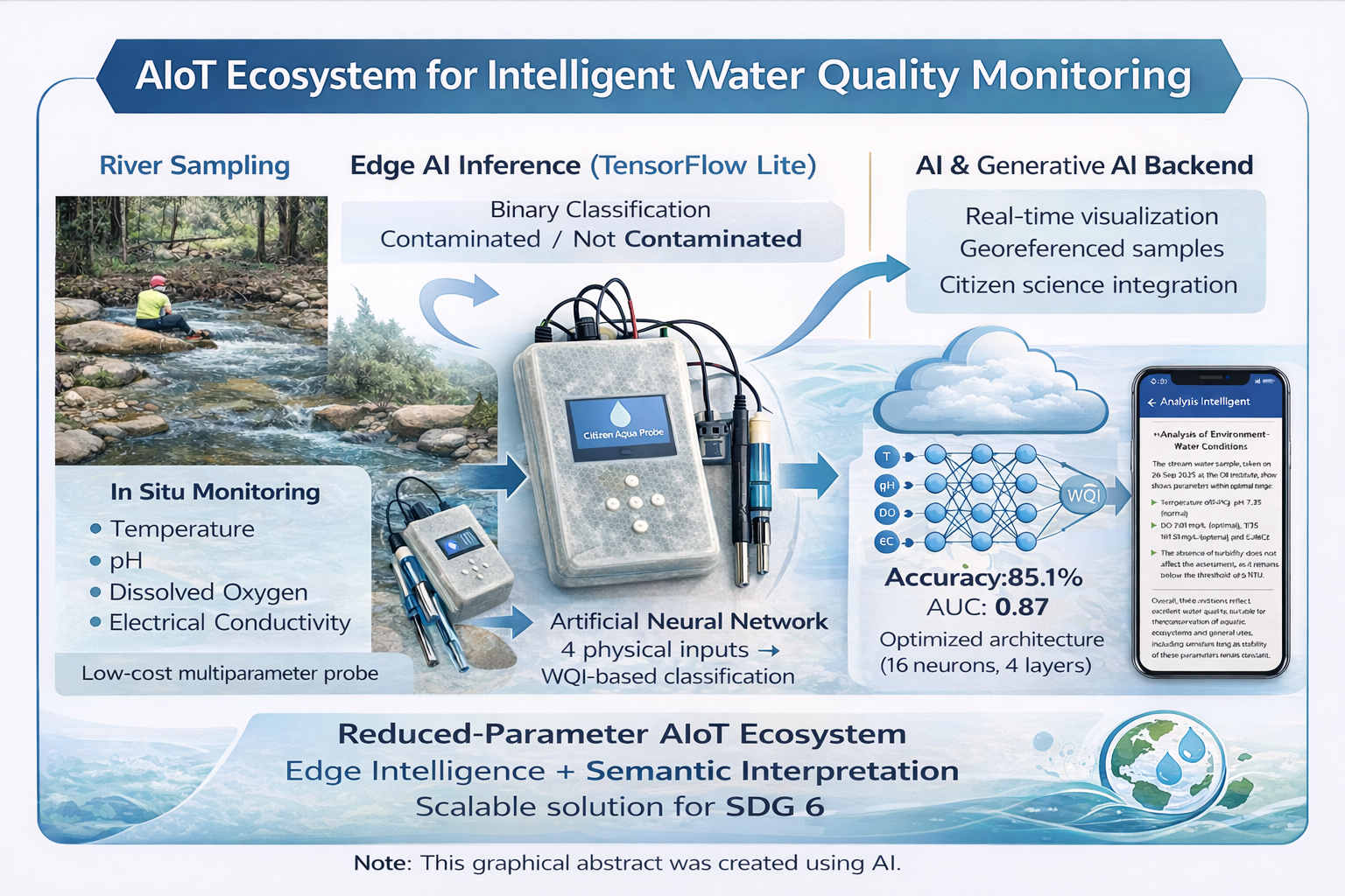
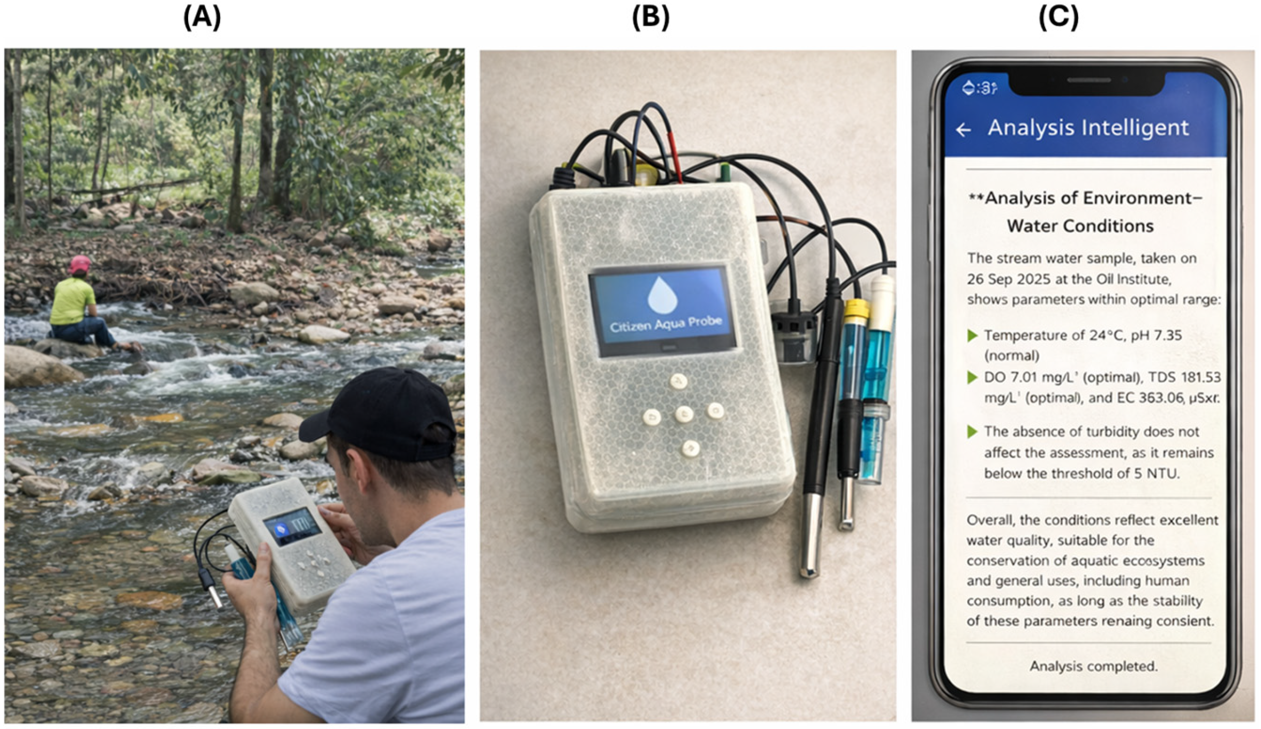
The experimental validation of the proposed AIoT ecosystem includes both field deployment and system-level integration. As illustrated in Figure 2, the system was evaluated through in situ measurements in riverine environments, the implementation of the multiparameter probe with embedded edge AI capabilities, and the generation of natural-language interpretations via the generative artificial intelligence module.

2.2.1. Dataset Description

A publicly available historical water quality dataset was used, derived from governmental measurements conducted in water bodies across India [14]. This dataset was selected for its temporal breadth and geographic diversity, encompassing multiple types of water sources. It contains records of seven essential physicochemical and biological parameters: Temperature, pH, Dissolved Oxygen (DO), Electrical Conductivity (EC), Biochemical Oxygen Demand (BOD), Nitrates, and Fecal Coliforms. These variables are critical both for calculating the target variable (WQI) and for training the neural network.

2.2.2. Missing Data Imputation (KNN)

In this study, the KNN imputation was implemented by selecting k = 5 nearest neighbors, a commonly adopted value that balances local sensitivity and robustness to noise. Prior to applying the imputation, all variables were normalized using Min–Max scaling to ensure that differences in measurement units and ranges did not bias the distance calculations.

The similarity between samples was computed using the Euclidean distance metric in the normalized feature space. For each missing value, the imputed value was estimated as the mean of the corresponding feature values from the k nearest neighbors.

This multivariate approach allows the preservation of inter-variable relationships within the dataset, ensuring that the imputed values remain physically consistent with the underlying environmental patterns.

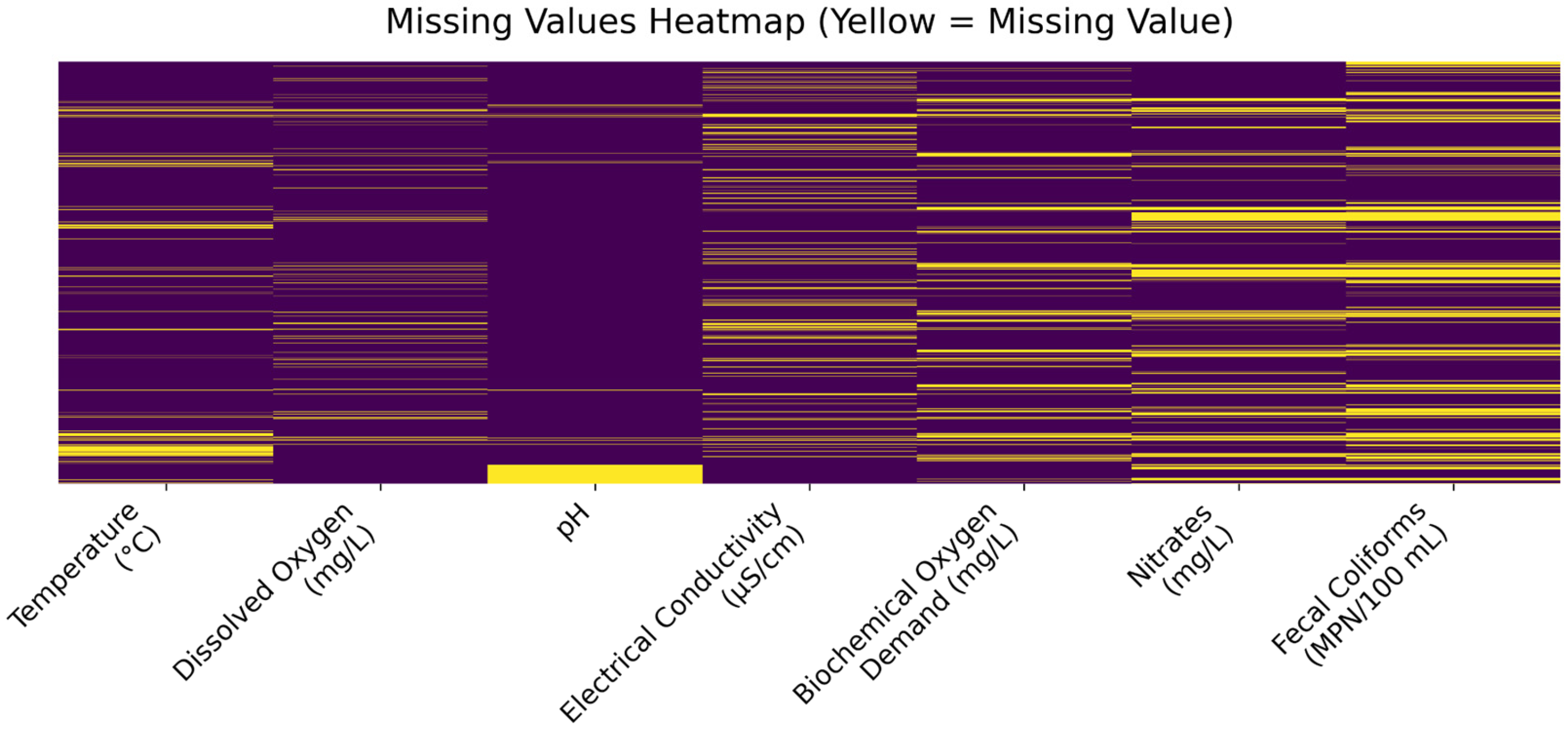
Exploratory analysis revealed the presence of missing values heterogeneously distributed across the dataset variables. Figure 3 illustrates this pattern, where yellow bands indicate the absence of records. This behavior is common in environmental monitoring systems, where factors such as sensor failures, transmission errors, or network issues generate information gaps. Such missingness affects critical calibration parameters, such as Temperature, and introduces bias into data analysis [3].

Completely removing these records would significantly reduce the effective sample size and could introduce additional bias, particularly in variables exhibiting temporal or environmental patterns. Although simple methods—such as mean or median substitution—are commonly used, they tend to reduce variance and ignore physical relationships among parameters, potentially distorting the system’s real behavior [15].

For these reasons, the K-Nearest Neighbors (KNN) Imputer algorithm was employed. This multivariate technique estimates missing values based on proximity between samples in feature space. This approach has demonstrated strong performance in contexts where parameters exhibit meaningful internal correlations, such as water quality studies and biomedical applications. In the environmental domain, prior research has shown that KNN imputation significantly improves predictive performance compared to deleting incomplete records, achieving accuracies of up to 0.99 when combined with multilayer models [16]. Similarly, in medical applications, KNN imputation has been reported to better preserve the covariance structure of datasets compared to univariate methods, resulting in substantial improvements in classification metrics [17].

Practically, KNN Imputer leverages known inter-variable relationships. For example, Temperature typically exhibits an inverse relationship with Dissolved Oxygen, and Electrical Conductivity often correlates with Dissolved Solids. By simultaneously considering multiple variables, this method reduces the risk of generating physically inconsistent values and helps maintain the dataset’s internal coherence.

2.2.3. Outlier Detection and Removal (IQR)

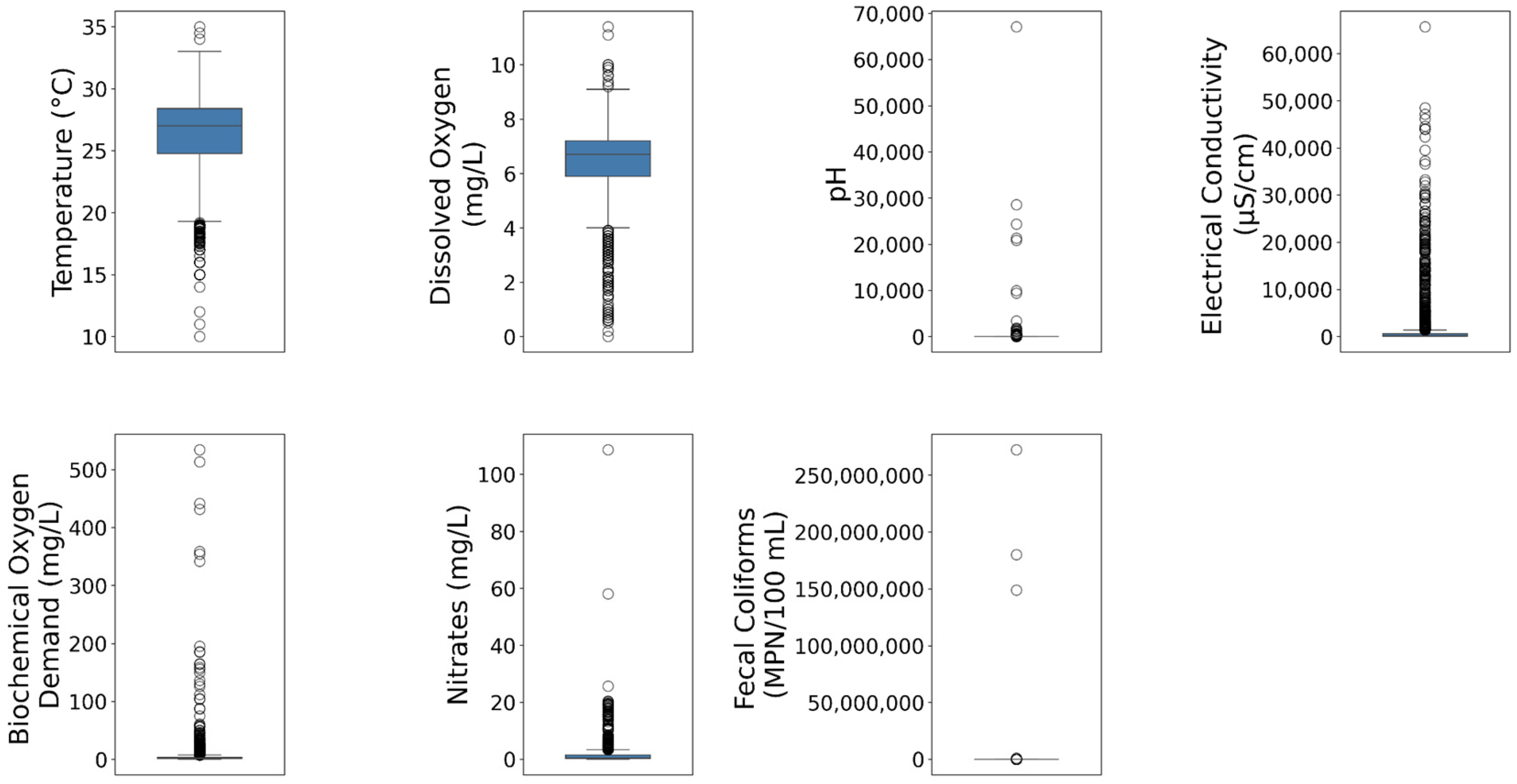
Due to the nature of in situ measurements, the dataset exhibited noise and extreme anomalies. A visual analysis using box-and-whisker plots (boxplots)—a tool recognized for its robustness in summarizing data dispersion and identifying extreme values without being influenced by them [18]—revealed significant deviations in parameters such as Fecal Coliforms and Electrical Conductivity that did not correspond to admissible natural variations (see Figure 4).

To mitigate the impact of these values on neural network training, the Interquartile Range (IQR) method was applied. The IQR is a statistical measure defined as the difference between the third quartile (Q3) and the first quartile (Q1), representing the central spread of the data [18]:

$$IQR = Q3 - Q1$$

(1)

Following Tukey’s standard methodology, data points located outside the intervals calculated using Equation (2) were defined as probable outliers [18].

$$[Q1-1.5·IQR, Q3+1.5·IQR]$$

(2)

This non-parametric approach is particularly suitable for environmental data because, as supported in the literature [18], the use of quartiles allows measurement noise to be filtered without being influenced by extreme values, unlike mean-based methods.

2.3. Target Variable Engineering: WQI Calculation

The adaptation of the Water Quality Index (WQI), based on the National Sanitation Foundation Water Quality Index (NSF-WQI), was driven by the operational constraints associated with real-time environmental monitoring using low-cost sensing devices. Specifically, parameters such as phosphates and turbidity were excluded, as their measurement typically requires laboratory-based analysis or specialized instrumentation that is not compatible with in situ, low-cost deployments.

The proposed system is conceived as a modular and scalable solution. The current implementation focuses on a subset of parameters that can be reliably measured using low-cost sensors, while maintaining the flexibility to incorporate additional variables in future system iterations, depending on the requirements of specific environmental or community contexts. Our previous work on low-cost water quality monitoring probes deployed in rural environments has demonstrated both the technical feasibility and practical applicability of such approaches [2,13,19,20,21].

To ensure methodological consistency, the weights of the remaining parameters were not arbitrarily modified. Instead, a proportional renormalization of the original NSF-WQI weights was performed. This approach preserves the relative importance assigned to each parameter in the standard formulation while ensuring that the total weight remains equal to one.

The subset of parameters used for WQI estimation includes key physicochemical and biological indicators, namely Dissolved Oxygen (DO), pH, Biochemical Oxygen Demand (BOD), Nitrates, Fecal Coliforms, Temperature, and Electrical Conductivity (used as a proxy for Total Dissolved Solids). These variables are widely recognized as representative descriptors of water quality in environmental monitoring studies.

This adaptation allows the WQI to remain conceptually aligned with its original formulation while enabling its application within low-cost, real-time monitoring frameworks.

For the generation of supervised labels, a unified quality index was computed. Although multiple indices are reported in the literature (e.g., CCME WQI, OWQI), the NSF-WQI was selected due to its generalized structure, ease of application, and broad validation for assessing surface water quality [22,23].

The standard NSF-WQI integrates physicochemical and biological parameters weighted according to their relative importance. The index is calculated as a weighted aggregation of sub-indices, normalized on a scale from 0 to 100, as defined in Equation (3) [22].

$$WQI=\sum _{i=1}^n{Q}_i\cdot W_i$$

(3)

where

• n is the total number of parameters considered.
• Q_i is the quality sub-index of the i-th parameter, obtained from standardized rating curves.
• W_i is the relative weight assigned to that parameter, such that: $\sum W_i=1$

Clarification on Data Origin for WQI Calculation: It is critical to distinguish the origin and application of the parameters detailed in

Table 1. Redistribution of Weights for the Adapted WQI Calculation.

Parameter	Original Weight (Worig)	Adjusted Weight (Wadj)
Dissolved Oxygen (%)	0.17	0.2020
Fecal Coliforms	0.16	0.1908
pH	0.11	0.1347
BOD	0.11	0.1347
Temperature (ΔT)	0.10	0.1234
Nitrates	0.10	0.1234
Total Solids (EC *)	0.07	0.0899
Phosphates	0.10	N/A
Turbidity	0.08	N/A
Total Sum	1.00	1.00

* Note: Electrical Conductivity (EC) was used as a proxy for Total Dissolved Solids.

. The original weights presented in the second column correspond to the standard NSF-WQI formulation, from which the seven parameters available in the historical dataset from India [14] were selected. Consequently, the adjusted weights in the right column were strictly applied to these seven dataset parameters (which include biological markers like Fecal Coliforms and BOD) to calculate the final target WQI labels for training. In contrast, the operational AIoT edge device only measures four physical parameters in real time (Temperature, pH, DO, and EC). The trained classification model is designed to infer the water quality status based solely on these four inputs, effectively bypassing the need for in-field biological sampling.

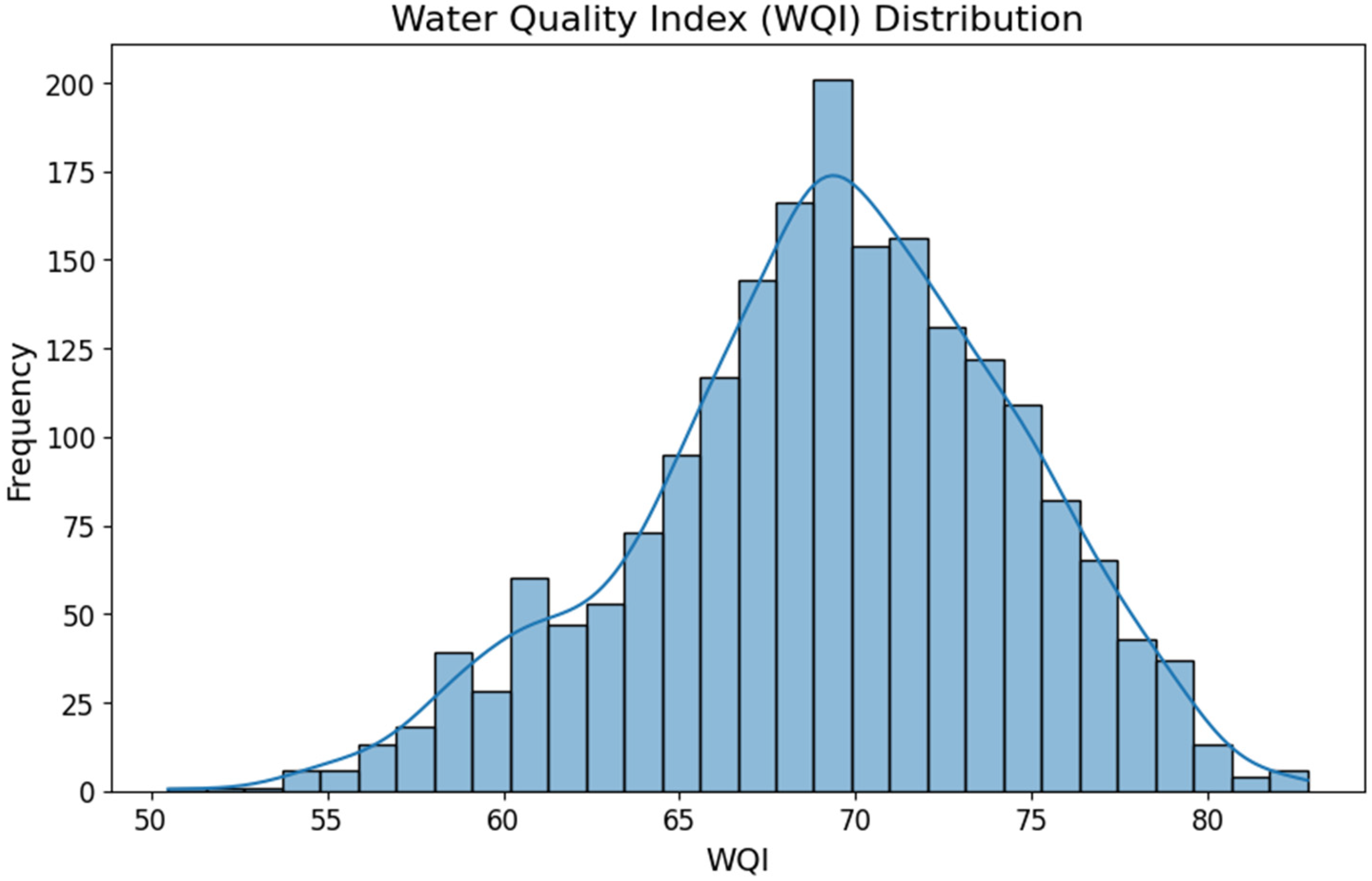
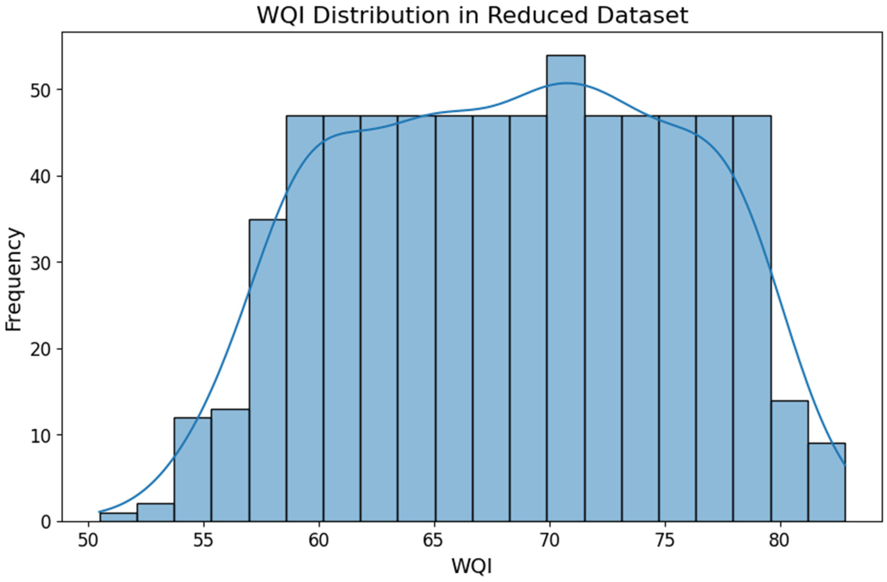
After applying Equation (3) with the adjusted weights described above, the labels for the dataset were generated. Figure 5 illustrates the statistical distribution of the resulting WQI.

The visual analysis shows a unimodal distribution centered approximately around a value of 70, covering an effective range between 50 and 83.

2.4. Experimental Design of the Classification Model

The central challenge stemmed from the input constraint imposed by the hardware. While the WQI calculation was based on seven physicochemical and biological parameters, the Artificial Neural Network (ANN) had to be trained using only the four variables that the physical probe can measure in situ: Temperature, pH, Dissolved Oxygen, and Electrical Conductivity.

This limitation required shifting from a regression approach to a binary classification framework, under the hypothesis that these four physical parameters contain sufficient information to discriminate the overall state of water quality.

2.4.1. Class Definition and Data Partitioning

The continuous target variable (WQI) was discretized by establishing a decision threshold at WQI = 70, following the NSF rating scale. This defined two mutually exclusive classes:

-

Not Contaminated (Class 0): Samples with WQI ≥ 70, indicating acceptable or good water quality.

-

Contaminated (Class 1): Samples with WQI < 70, indicating significant deterioration.

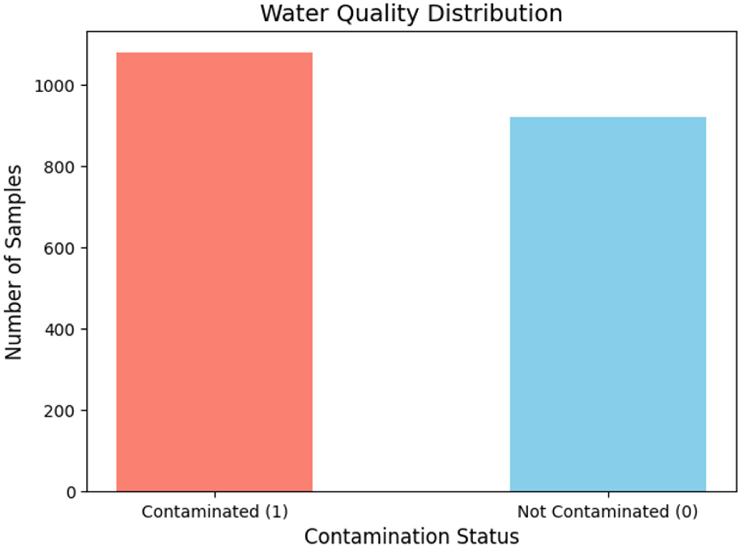
Figure 6 shows the frequency distribution of these two classes in the dataset prior to balancing. For model validation, the dataset was randomly divided into two subsets: 80% for training and 20% for testing (hold-out), maintaining stratification to preserve the original class proportions.

To ensure reproducibility of the experimental design, a fixed random seed (random_state = 42) was used during dataset partitioning. This guarantees that the training–testing split and class distribution remain consistent across different runs.

Furthermore, the same random seed was maintained across all experimental scenarios to ensure comparability of results and avoid variability due to random sampling.

Grid Search ensures identification of the best possible configuration within the predefined search grid, eliminating arbitrariness in network design.

The optimization was performed using 5-Fold Cross-Validation to ensure that the results were generalizable and not dependent on a specific data partition, a methodology commonly employed for tuning predictive water quality models [24].

Table 2. Hyperparameter Search Space for the Neural Network.

Hyperparameter	Explored Values
Neurons per hidden layer	16, 32, 64
Number of hidden layers	1, 2, 4, 6
Activation function	ReLU, Tanh
Learning rate	0.001, 0.01
Batch size	16, 32
Epochs	100 (fixed)

details the explored hyperparameter search space.

2.4.2. Evaluation Metrics

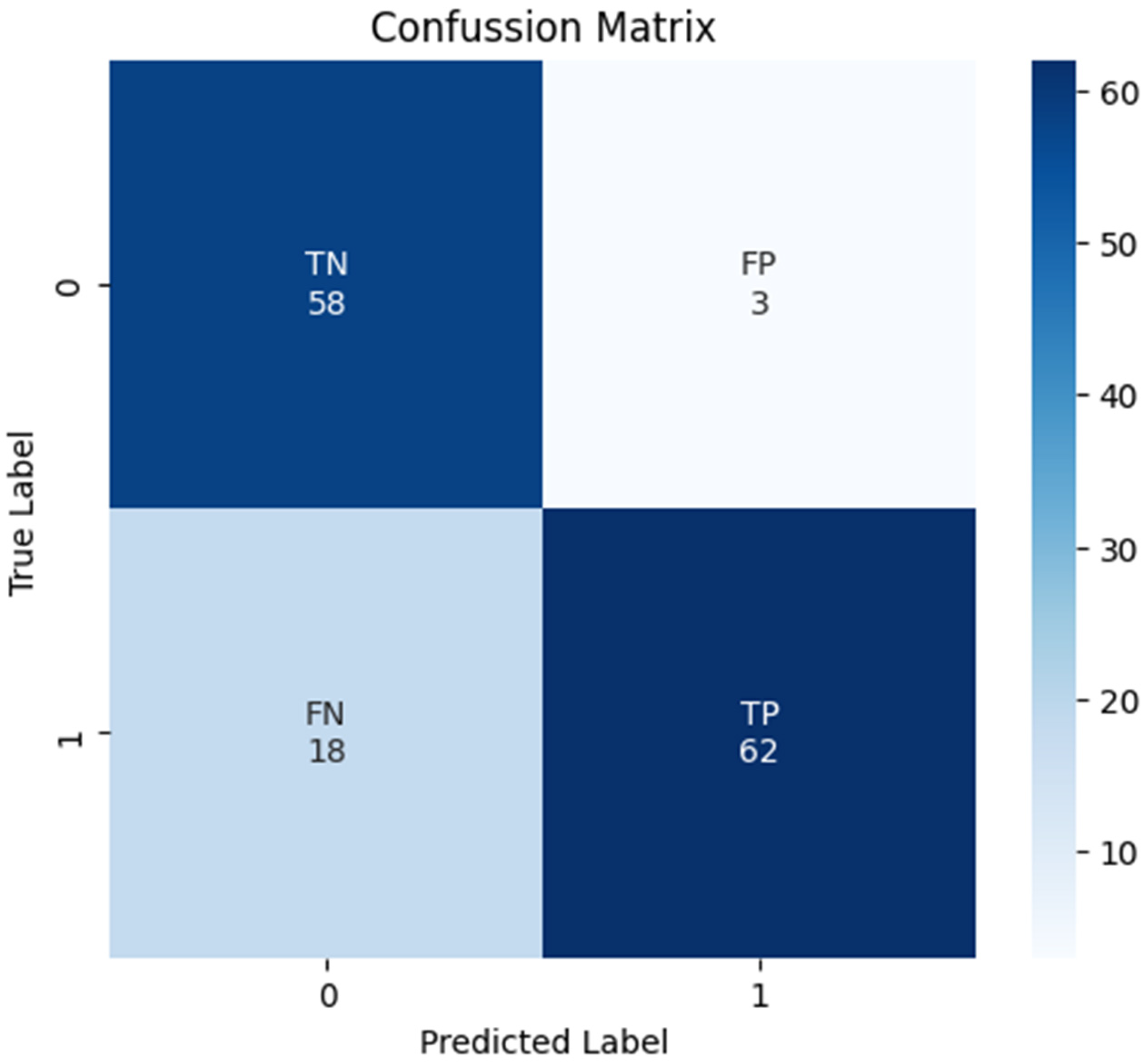
The performance evaluation of the binary classification models was based on the analysis of the confusion matrix, composed of True Positives (TP), True Negatives (TN), False Positives (FP), and False Negatives (FN) [25,26].

Although model selection considered Accuracy as a global metric, the recent literature warns that this measure may yield overly optimistic results in imbalanced datasets, as it can be dominated by the majority class [25,26].

Therefore, to ensure a robust and consistent evaluation under possible variations in class prevalence [26], complementary metrics were also recorded, including Precision, Recall, F1-Score, and AUC:

Accuracy: Proportion of correct predictions over the total number of cases [22].

$$Accuracy={\displaystyle \frac{TP+TN}{TP+TN+FP+FN}}$$

(4)

Precision: The model’s ability to avoid labeling a negative sample as positive. Also known as Positive Predictive Value (PPV) [23].

$$Precision={\displaystyle \frac{TP}{TP+FP}}$$

(5)

Recall (Sensitivity): The model’s ability to correctly identify all positive samples, which is crucial to avoid missing true contamination events. Mathematically equivalent to the True Positive Rate (TPR) [25].

$$Recall={\displaystyle \frac{TP}{TP+FN}}$$

(6)

F1-Score: The harmonic mean of Precision and Recall. It is commonly used when seeking a balance between both metrics, although it does not consider true negatives in its formulation [17].

$$F1={\displaystyle \frac{2\cdot TP}{2\cdot TP+FP+FN}}$$

(7)

ROC Curve (Receiver Operating Characteristic): A graphical representation illustrating the diagnostic ability of a binary classifier as its discrimination threshold varies, plotting TPR against the False Positive Rate (FPR) [26].

AUC (Area Under the ROC Curve): A scalar metric that quantifies the area under the ROC curve. Recent studies highlight AUC as one of the most consistent metrics for evaluating and comparing models independently of class prevalence [18]. It represents the probability that the model assigns a higher score to a randomly chosen positive example than to a randomly chosen negative one [26].

An AUC value close to 1 indicates excellent performance, whereas a value of 0.5 suggests performance equivalent to random guessing.

Matthews Correlation Coefficient (MCC): Introduced to provide a balanced measure of quality for the binary classification, especially robust in scenarios with potential class imbalances. It considers all four confusion matrix categories (TP, TN, FP, FN) [25].

$$MCC={\displaystyle \frac{TP\cdot TN-FP\cdot FN}{\sqrt{(TP+FP)(TP+FN)(TN+FP)(TN+FN)}}}$$

(8)

2.4.3. Experimental Scenarios

To validate the research hypothesis and progressively improve model performance, four incremental training scenarios were designed and evaluated. The mathematical and methodological configuration of each is detailed below:

Scenario 1 (Baseline): Training was conducted using the complete original dataset. Only the four base parameters were used as the input vector, and no balancing preprocessing was applied. This scenario establishes reference performance.

Scenario 2 (Feature Engineering): The input space was enriched to capture nonlinear relationships. From the original variables, an extended feature space $X_{ext}$ was generated by applying polynomial, inverse, and logarithmic transformations (using $ln(1+x)$ to handle zeros), as well as second-order interaction terms. The new features were defined as follows:

$$X_{poly} = \{T^2,C{E}^2, p{H}^2, T^{-1},p{H}^{-1}\}$$

(9)

$$X_{log}=\left\{ln\right(1+T), ln(1+CE), ln(1+pH\left)\right\}$$

(10)

$$X_{inter}=\{T\cdot pH, pH\cdot CE, T\cdot CE\}$$

(11)

The final input vector for this scenario is the union of these sets

$$X_{final}=X_{base}\cup X_{poly}\cup X_{log}\cup X_{inter}$$

Scenario 3 (Balancing and Stratified Sampling): Class imbalance was addressed using a density-based stratified subsampling strategy. The procedure was formalized as follows:

-

Class Definition: A binary threshold was established such that $y = 1$ (Contaminated) if $WQI < 70$, and $y = 0$ otherwise.

-

Discretization: To preserve the data structure, the continuous WQI range was divided into 20 intervals (bins).

-

Selection: The dataset was reduced to approximately $N\approx N_{total}/2$. Samples were randomly selected within each group defined by the intersection $\left(Bi{n}_{WQI}\cap Class\right)$, ensuring continuity of the distribution as illustrated in Figure 7.

Scenario 4 (Combined Approach): Integration of strategies. The balanced dataset resulting from Scenario 3 was used as the training base, while feeding the neural network with the extended feature vector $X_{final}$ developed in Scenario 2. This approach aims to maximize both generalization capacity under class imbalance and sensitivity to complex nonlinear patterns.

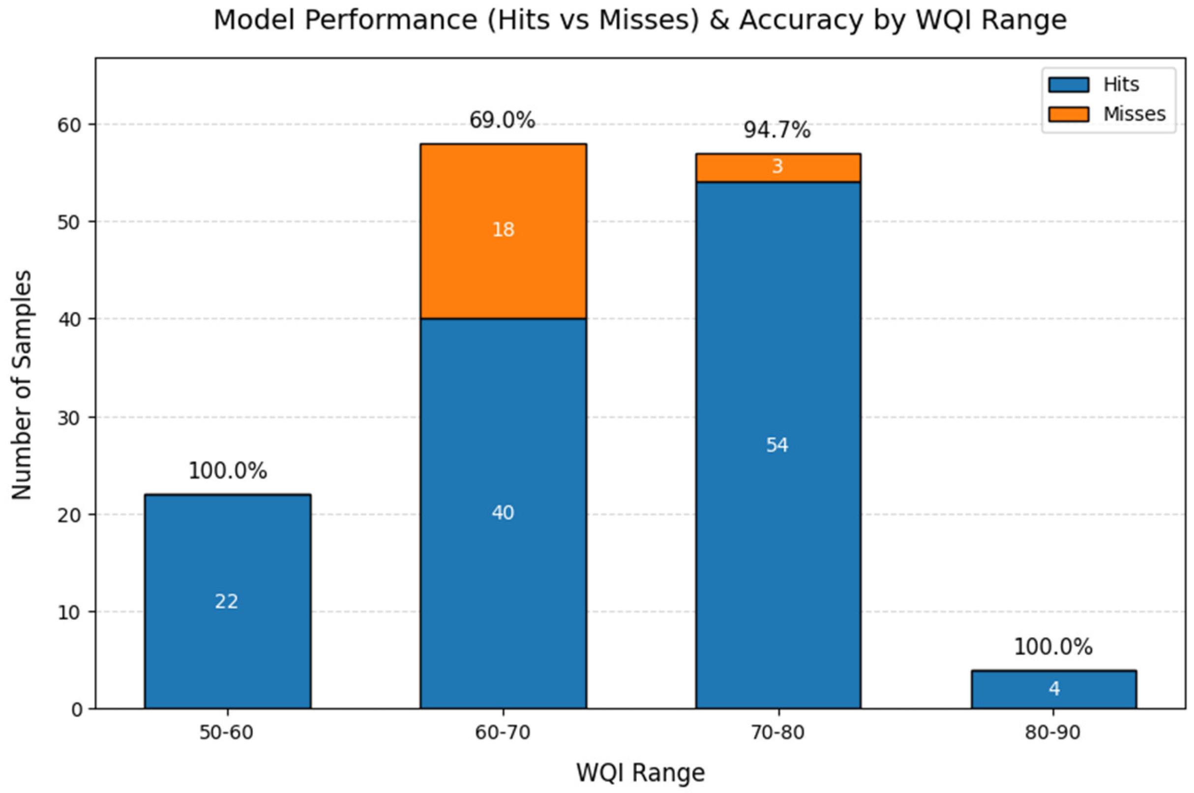
Finally, to comprehensively evaluate the classification behavior of the optimal model across different contamination severity levels, a stratified performance analysis was conducted. This post hoc evaluation quantifies the proportion of correct and incorrect predictions within predefined WQI intervals (e.g., 50–60, 60–70), allowing the identification of potential performance variations near decision boundaries.

2.5. Mobile Platform and Cloud Services

The Water Probe Hub application acts as the integration hub of the ecosystem, evolving from a standard visualization interface into a comprehensive data management and citizen science tool.

2.5.1. Data Management and Connectivity

The application implements a service discovery protocol over Bluetooth Low Energy (BLE) to identify and pair with multiparameter probes. Once the connection is established, the monitoring module displays real-time parameter readings and manages sample acquisition.

To ensure spatial traceability, a hierarchical storage structure based on “batches” was designed. Each captured sample is automatically labeled with geospatial metadata (latitude and longitude) obtained from the mobile device’s GPS sensors. This georeferencing is fundamental for contamination mapping and subsequent spatial trend analysis.

2.5.2. Citizen Science Module

To democratize access to environmental information, a community module was integrated. This functionality allows users to publish their sample batches in an open repository, promoting collaboration and data transparency. The interface enables visualization of public batches from other users, fostering interaction and the collective construction of water quality maps, in alignment with participatory citizen science paradigms.

2.5.3. Generative Analysis Architecture (Backend)

Beyond local binary classification, the system incorporates an advanced semantic analysis layer hosted in the cloud. The backend, developed using the Fast API framework, acts as an intermediary for data management, database communication, and interaction with Generative Artificial Intelligence providers.

This service receives the sample’s feature vector and constructs a structured prompt that includes geographic context and physicochemical values. The architecture is designed to be model-agnostic, allowing flexible integration with different Large Language Models (LLMs). The backend processes the LLM response and returns to the application a descriptive natural-language analysis explaining potential causes of detected contamination and their ecological implications.

To standardize the LLM’s interpretation, the exact prompt architecture used is defined as follows:

• [Context and Metadata]
• Environmental/Water Conditions Analysis
• Location: {sample_location} | Time: {formatted_time} | Origin: {sample_origin}
• [Monitoring Data]
• Temperature: {temperature} °C
• Dissolved Oxygen (DO): {do} mg/L
• TDS: {tds} mg/L
• pH: {ph} pH Units
• Electrical Conductivity (EC): {ec}
• [Instructions]

• Generate a concise analysis of the conditions in a single paragraph (maximum 5 to 8 lines).
• Interpret only the present values (omit NA or nulls) and classify each parameter according to typical water quality ranges:

  -

  pH: 6.5 to 8.5 → normal

  -

  DO: >5 mg/L → optimal, 3 to 5 → warning, <3 → critical

  -

  TDS: <500 mg/L → optimal, 500 to 1000 → normal, >1000 → warning

  -

  EC: 0 to 500 μS/cm → optimal, 500 to 1500 → normal, >1500 → warning

• Indicate whether the overall water conditions appear optimal, warning, or normal for a typical aquatic ecosystem and for general use or human consumption.
• Use the origin and location of the sample as context if available.
• Use concise technical language, avoiding mention of missing data and overly generic terms.

3. Results

3.1. Evaluation of Classification Performance

The experimental validation of the Artificial Neural Network (ANN) was conducted under a critical information constraint: while the Ground Truth (WQI) calculation integrates seven physicochemical and biological parameters, the predictive models were trained and evaluated using exclusively the four input variables available from the physical probe (Temperature, pH, Dissolved Oxygen, and Electrical Conductivity).

This mismatch imposes a significant challenge, requiring the model to infer latent contamination patterns without direct access to determinant variables such as BOD or fecal coliforms.

Performance was progressively evaluated across the four defined scenarios.

Table 3. Performance Metrics Comparison of the Best Models per Scenario (Test Set).

Scenario	Optimal Configuration	MCC	Accuracy	Precision	Recall	F1-Score	AUC
1. Baseline	[64 N, 6 L, ReLU]	0.5656	0.7845	0.7843	0.7845	0.7844	0.86
2. Feature Engineering	[16 N, 6 L, ReLU]	0.5858	0.7945	0.7943	0.7945	0.7944	0.86
3. Data Balancing	[32 N, 4 L, Tanh]	0.7212	0.8511	0.8714	0.8511	0.8515	0.86
4. Combined (Final)	[16 N, 4 L, Tanh]	0.7212	0.8511	0.8714	0.8511	0.8515	0.87

Note: N = Neurons per layer, L = Hidden layers.

summarizes the metrics obtained on the independent test set for the best model identified in each scenario through Grid Search.

3.1.1. Training Dynamics and Generalization Analysis

To further assess model stability and potential overfitting, the training and validation loss curves of the final ANN configuration (16 neurons, 4 hidden layers, tanh activation) were analyzed, as shown in Figure 8.

The loss curves exhibit a rapid decrease during the first five epochs, followed by a smooth and monotonic convergence toward stability. Notably, the validation loss remains consistently below the training loss throughout the optimization process. This behavior suggests effective regularization and absence of overfitting, which is further supported by the negative overfitting gap (−0.0517) observed in the test evaluation.

The smooth convergence and minimal divergence between training and validation curves confirm that the model achieves stable learning dynamics and maintains strong generalization capability despite the reduced dimensionality of the input feature space.

The results indicate that the preprocessing strategies had a differentiated impact on model performance: The comparative analysis reveals that the preprocessing strategy had a hierarchical impact on performance:

-

Impact of Data Balancing (Scenario 3): This was the most influential factor. By correcting the majority-class bias through stratified sampling, an improvement of 6.66% in both Accuracy and F1-Score was achieved compared to the baseline. This suggests that, in imbalanced environmental datasets, model performance is strongly influenced by the quality and representativeness of the training data distribution.

-

Effectiveness of Feature Engineering (Scenario 4): Although Accuracy remained stable relative to Scenario 3, the integration of nonlinear features (polynomial terms and interactions) increased the Area Under the ROC Curve (AUC) to 0.87. As shown in Figure 9, the Scenario 4 model (red curve) exhibits greater convexity in the upper-left region compared to the baseline (blue curve), indicating improved discrimination capability at critical decision thresholds and reduced false positives.

-

Furthermore, the Matthews Correlation Coefficient (MCC) was used as a robust evaluation metric. The baseline model (Scenario 1) achieved an MCC of 0.5656, indicating moderate predictive performance. In contrast, the final combined model (Scenario 4) reached an MCC of 0.7212. This improvement highlights the model’s better capability to classify both contaminated and non-contaminated instances in a balanced manner, even under the complexities of the reduced feature space.

-

Computational Efficiency: A relevant finding is the reduction in model complexity. While the baseline required 64 neurons and 6 hidden layers to reach 78% Accuracy, the final model (Scenario 4) achieved 85.1% with a lighter architecture of only 16 neurons and 4 hidden layers. This compactness is essential for deployment on mobile and embedded devices (Edge AI), reducing computational load without sacrificing performance.

Figure 10 presents the Confusion Matrix of the final model (Scenario 4). Notably, the system minimizes False Positives (only 3 cases out of 141 test samples), a desirable characteristic to avoid unnecessary alarms that could reduce user trust. At the same time, the model maintains strong capability in detecting real contamination events (62 True Positives), validating its usefulness as an early-warning tool despite the limitation in input parameters.

The robustness of the AIoT ecosystem was validated through heterogeneous deployment, executing the optimized model (Scenario 4) on two distinct processing nodes: the embedded firmware of the probe and the mobile application. This dual implementation ensures operational redundancy and prediction availability regardless of the visualization interface.

Figure 11 presents empirical evidence of performance in both environments. The left panel shows the probe’s debugging interface, highlighting a recorded inference time of 0 ms. This result confirms that the compact neural network architecture (16 neurons, 4 hidden layers) is lightweight enough to operate nearly in real time on the probe, considering a sampling period of 1 s and processing the four input parameters (Temperature, EC, DO, pH) without perceptible latency.

Simultaneously, the central and right panels illustrate the response within the mobile application. The model translates output probabilities into visual indicators for user interpretation. The consistency between the probe’s prediction and the application’s output validates the correct quantization and export of the model into TFLite format, ensuring uniform decision logic across the entire ecosystem.

3.1.2. Stratified Performance Analysis

To further evaluate the model’s robustness and characterize its behavior across different contamination levels, a stratified analysis was conducted over four WQI ranges (50–60, 60–70, 70–80, and 80–90). Figure 12 illustrates the proportion of correct predictions (hits) versus misclassifications (misses), along with the overall accuracy within each interval.

The results show that the model achieves a classification accuracy of 100.0% at the extremes of the spectrum (50–60 and 80–90). This suggests that moderate contamination and good water quality conditions can be distinguished with relative ease using only the four physical parameters (Temperature, pH, DO, and EC). The lowest accuracy (69.0%) is observed in the 60–70 range, immediately below the classification threshold (WQI = 70). This behavior is consistent with expectations, as samples near the decision boundary exhibit subtle physicochemical variations that may hinder discrimination without the use of additional biological and chemical indicators (e.g., BOD or fecal coliforms).

In the 70–80 range, the model achieves an accuracy of 94.7%, suggesting good performance in identifying acceptable water quality conditions. Overall, this stratified analysis indicates that the edge AI approach may be useful in early-warning scenarios, although with greater uncertainty around the decision boundary.

4. Discussion

4.1. Comparison with Prior Work

Recent studies and reviews show that machine learning models for water quality prediction typically achieve accuracy values above 85% and AUC values close to 0.90 when trained on large datasets that include multiple physicochemical and biological parameters [27,28]. However, these approaches generally rely on laboratory-derived variables and centralized (cloud-based) processing, which limits their applicability under real-time field conditions.

Similarly, approaches that combine machine learning with remote sensing offer robust predictive capabilities at larger spatial scales, but they depend on indirect estimations and more complex processing, making them less suitable for in situ monitoring [29].

Furthermore, recent work on AI-based water quality assessment highlights improvements in predictive performance, but still points to challenges related to real-time implementation, system integration, and interpretability for end users [30].

Edge-based approaches have been increasingly explored; however, many implementations remain limited by model complexity or lack of real-world validation [28,31].

In contrast, the system proposed in this study achieves competitive performance (accuracy = 85.1%, AUC = 0.87) using only four directly measurable variables (temperature, pH, dissolved oxygen, and electrical conductivity). This reduced set of inputs enables a more practical and scalable implementation compared to approaches that require extended parameter sets.

A key contribution of this work is the deployment of artificial intelligence at the edge. The model is implemented using TensorFlow Lite directly on the sensing device and mobile application, enabling real-time inference with sub-millisecond latency. This eliminates dependence on continuous network connectivity and significantly improves responsiveness in field conditions.

From a practical perspective, the results highlight a trade-off between model complexity and deployability. While models using a larger number of variables may achieve slightly higher predictive performance, they are often not suitable for real-time, low-cost monitoring in rural or resource-constrained environments.

These results demonstrate that reliable water quality classification can be achieved with a reduced number of variables and real-time edge inference, supporting its practical deployment in decentralized environmental monitoring systems.

4.2. Generative AI and Citizen Science

While edge inference provides an immediate binary alert, the cloud-based Generative Artificial Intelligence layer addresses the need for interpretability. The textual analysis generated by the LLM demonstrates multidimensional synthesis capability that goes beyond simple threshold verification. As illustrated in Figure 11, the system:

-

Contextualizes physical parameters: It does not merely report raw values (T = 24.27 °C, pH = 7.35, DO = 7.01 mg/L), but qualitatively labels them as normal or optimal based on environmental standards embedded within the system prompt.

-

Integrates complex variables: It correlates Electrical Conductivity (363.06 μS/cm) and Total Dissolved Solids (181.53 mg/L) to rule out significant turbidity, inferring water transparency.

-

Provides an overall qualitative assessment: The model generates an integrated interpretation of water quality conditions (e.g., “excellent quality” as displayed in the application Figure 11), which should be understood as an indicative early-warning assessment based on the available parameters, rather than a comprehensive environmental certification. Such comprehensive evaluations typically require laboratory-based analyses, controlled sampling protocols, and extended processing and interpretation stages, which may be difficult to implement in real-time and resource-constrained rural contexts. The model concludes with an overall assessment (excellent quality), explicitly suggesting the suitability of the water body for ecosystem conservation and general uses.

This functionality transforms the device from a purely technical measurement instrument into an educational tool. By translating complex numerical vectors into natural language, the system reduces the cognitive barrier for non-expert users, facilitating community participation and fostering citizen science.

It is important to emphasize that the interpretations generated by the system are based on a reduced set of physicochemical parameters (temperature, pH, dissolved oxygen, and electrical conductivity), which, although informative, do not capture all potential contamination sources, such as heavy metals, pesticides, or emerging pollutants.

Therefore, the outputs provided by the system should be understood as indicative early-warning assessments intended to support rapid field diagnostics and community awareness, rather than as comprehensive environmental certifications. In this context, statements such as “excellent water quality” should be interpreted as relative to the measured parameters and not as definitive evidence of overall ecosystem suitability.

Comprehensive water quality evaluations require laboratory-based analyses, controlled sampling protocols, and a broader set of physicochemical and biological indicators. Accordingly, the proposed system is designed to complement, rather than replace, conventional monitoring approaches, particularly in resource-constrained and real-time monitoring scenarios.

In addition, the proposed approach contributes to bridging the gap between data acquisition and actionable knowledge, particularly in rural and resource-constrained environments, where accessibility and interpretability are critical factors for adoption.

Future work should focus on integrating additional sensing capabilities and hybrid monitoring approaches, as well as validating the system across diverse environmental conditions, to improve diagnostic completeness and robustness.

5. Conclusions

The experimental evidence demonstrates that a limited set of four physical parameters (Temperature, pH, Dissolved Oxygen, and Electrical Conductivity), measurable using low-cost sensors, contains sufficient latent information to effectively infer the presence of complex biological and chemical contamination. The developed Artificial Neural Network model successfully reconstructed the decision logic of the NSF-WQI index—which theoretically requires up to nine variables—achieving an accuracy of 85.1% and an AUC of 0.87.

Optimization of the network architecture (16 neurons, 4 hidden layers) demonstrated that computational intelligence can be efficiently implemented at the edge (probe and mobile application). With inference times below 1 ms and minimal memory usage, real-time diagnostic capability was achieved without requiring permanent cloud connectivity, enabling deployment in rural or remote areas.

Finally, integrating this predictive model with Generative Artificial Intelligence capabilities redefines the role of environmental instrumentation. The probe evolves from a passive device for raw data collection and visualization into an intelligent agent capable of interpreting environmental conditions through its integration with the mobile ecosystem. Beyond providing binary classification, the system delivers semantic context regarding potential causes and ecological implications through natural language explanations. In doing so, the ecosystem empowers end users, bridging the gap between technical measurements and public understanding, thereby fostering informed decision-making and participatory environmental monitoring.

In subsequent stages, a relevant line of work involves the development of a local dataset in Colombia. This would enable analysis of the extent to which patterns learned from historical water body data in other countries are transferable. In this context, transfer learning techniques could be employed to adapt previously trained models and evaluate whether the relationships between physicochemical variables and the WQI remain consistent under different climatic and geological conditions.

Although binary classification is useful for early warning systems, environmental management applications often require direct estimation of the water quality index. Therefore, future work also includes exploring low-complexity regression models capable of predicting the scalar WQI value (0–100), while maintaining a reduced input set suitable for edge devices.

Currently, the system operates under a point-based diagnostic approach. A potential extension involves incorporating temporal models, such as LSTM or GRU architectures, capable of processing historical time series from each sampling location. This would enable predictive capabilities, allowing anticipation of deterioration trends before critical thresholds are exceeded.