A Lightweight Python Recovery Tool for Waveform Gap Recovery in Seismic–Volcanic Monitoring Networks

Abstract

Seismic–volcanic monitoring networks often operate in remote areas over heterogeneous links (e.g., microwave radio and cellular). During event-driven seismic episodes, sustained multi-station waveform streams can stress both last-mile connectivity and data acquisition systems, yielding discontinuities in center-side archives even when stations keep recording locally. This paper presents the Python Recovery Tool (PRT), a lightweight command-line artifact that retrieves buffered waveform files after reconnection and rebuilds daily archives that can be ingested by the monitoring center without hardware upgrades. PRT detects archive gaps from daily (Julian day) file partitions and embedded timestamps, and reduces recovery traffic by selectively fetching only the files needed to backfill missing intervals. We evaluated PRT on five event-driven recovery cases using operational file-based evidence from station and center listings complemented with a simple bandwidth-based recovery-time model. Across the cases, PRT restored archive continuity while reducing download volume by 4.43–93.75% relative to naive bulk retrieval, with modeled catch-up times ranging from 0.79 to 207.59 min, depending on station-side packaging granularity and bottleneck link capacity. These results support a practical retrofit path to improve archive completeness under constrained links and heterogeneous deployments.

1. Introduction

Seismic and volcanic monitoring networks aim to deliver continuous data streams to a data and interpretation center for analysis and decision making [1]. Many stations are installed in remote areas and depend on heterogeneous communication links. These links often include microwave segments (Wi-Fi, satellite, cellular data, among others) and, in some cases, fiber optics. Link quality can degrade due to limited coverage, harsh weather, power constraints, and reduced infrastructure [2,3]. As a result, transmissions may become unstable, and the data center receives an incomplete time series.

Monitoring centers commonly rely on acquisition and processing platforms to store continuous data and support near real-time products [2,4]. Examples include SeisComP, Antelope, and Earthworm. When the communication path is interrupted, missing segments appear in waveform archives. These gaps reduce the value of the records for later tasks, affecting reprocessing, event classification, and long-term analysis [5]. In operational contexts, gaps also complicate quality control: they can be confused with low signal levels or acquisition problems, increasing manual work for operators.

The problem is more critical in multiparametric monitoring. A seismic–volcanic network can include sensors for velocity, acceleration, deformation, gas, temperature, and other parameters. Each subsystem may use different digitizers, formats, and proprietary tools [6,7,8]. Operators often need to correlate parameters to interpret unrest episodes and separate volcanic processes from tectonic activity [9]. If data gaps occur during relevant episodes, the reliability of these correlations can be reduced, limiting scientific interpretation. Although monitoring infrastructures are multiparametric, in this work, we focus on recovering waveform streams (e.g., seismic velocity, acceleration, and infrasound) that are central to event analysis and reprocessing; the proposed workflow can be extended to additional sensor products when similar buffer and archive conventions are available.

Several approaches exist to mitigate these gaps, including reconstruction methods and generic recovery strategies in sensor networks [10,11]. However, in many seismic monitoring networks, the most valuable information is the original waveform and its metadata. Recovering the original data after a link outage is therefore preferable to reconstructing missing segments. In many operational deployments, stations continue to record during a communication outage and temporarily store data locally. After reconnection, many deployments lack a practical and bandwidth-efficient mechanism to backfill the accumulated backlog into the acquisition archive. While acquisition stacks can ingest late data, the missing step is often the operational glue required to (i) identify the exact missing time spans at the archive level, (ii) map them to vendor-specific buffer layouts and file naming conventions at remote stations, (iii) screen candidates for existence/integrity to avoid re-sending corrupted or duplicate content, and (iv) rebuild standard daily archive units that the center can ingest without manual intervention. In such settings, generic file-transfer scripts are insufficient because they do not provide time-aware selection, format-preserving packaging, and idempotent reinjection aligned with the archive partitioning. Vendor upgrades may exist, but they can be costly and hard to deploy at scale across heterogeneous legacy equipment and mixed technologies. This motivates a low-cost retrofit solution that can operate with proprietary data organization and constrained links.

This paper presents a Python-based software tool for waveform gap recovery in seismic–volcanic monitoring networks. The tool supports the retrieval of buffered records after reconnection and follows a minimal overhead strategy to reduce channel usage when bandwidth is limited. We evaluate the approach using operational evidence from event-driven windows and a parametric analysis of recovery time under heterogeneous link capacities.

The main contributions are as follows: (i) a retrofit recovery workflow and implementation that maps archive-level gaps to station-side buffered files and reinjects rebuilt daily waveform archives into the acquisition center; (ii) a compact evaluation framework based on archive time availability and dump-relative transmission savings; and (iii) an operational assessment across five event-driven cases, including a bandwidth-based recovery time analysis under constrained effective throughput.

The rest of the paper is structured as follows: Section 2 describes the system context and the problem. Section 3 summarizes related work. Section 4 describes data organization, gap identification, and the role of proprietary records. Section 5 presents the artifact design. Section 6 explains the evaluation methodology. Section 7 reports results. Finally, Section 8 concludes the paper. Appendix A, Appendix B and Appendix C present the storage structure, mapping rules, and pseudocode of the retrieval flow, providing the technical details that ensure its correct implementation and reproducibility.

2. Background and Problem Statement

2.1. Monitoring Network Context

Seismic and volcanic monitoring is commonly operated by seismological data centers (SDCs), which integrate acquisition, processing, storage, and dissemination services [1,4,7]. As networks evolve, SDCs incorporate new stations, repeater nodes, and processing capabilities, increasing the heterogeneity of the system.

From the perspective of post-outage continuity, a monitoring system can be viewed as a chain where discontinuities may appear and persist: (i) monitoring stations (sensors, digitizers, local storage, communications, power); (ii) transmission networks (radio/satellite/fiber segments, routers, repeaters, gateways); (iii) the data center (acquisition servers and archives for real-time products and reprocessing); and (iv) diffusion services (alerts and reports) [12]. Even when stations keep recording locally, missing segments may remain visible at the center-side archive after connectivity resumes, motivating explicit backfilling.

2.2. Communication Media and Availability Challenges

Seismic station data are commonly transferred over heterogeneous media. Typical links include microwave radio, satellite segments, cellular networks (3G/4G), and, in some deployments, optical fiber [12,13,14]. To extend coverage, many topologies incorporate repeater nodes and mixed media, improving reach but introducing multiple points of failure.

Data transfer may become discontinuous due to external and internal factors. External factors include radio-frequency interference and weather effects on wireless links. Internal factors include transmission equipment limitations, power backup failures, hardware faults, and delays or failures in acquisition-side retrieval and ingestion processes. Operational technical reports from monitoring networks in the region describe periods in which transmission performance remains below desired targets [15,16], which constrains early warning, rapid interpretation, and later reprocessing tasks [17,18]. In practice, such discontinuities manifest as missing intervals in center-side archives, even when corresponding data still exists in station-side buffers.

2.3. Information Gaps and Buffered Data

We use the following terms:

• Outage: a time interval during which the station cannot deliver data to the acquisition center.
• Gap: the missing interval observed in the acquisition archive at the data center.
• Backlog: the amount of data accumulated locally at the remote station during an outage, limited by local buffering capacity.

Many stations keep recording during an outage and store records locally for a limited time (disk, temporary buffer, or vendor-specific store). Because buffering is finite, long outages may cause older records to be overwritten or become inaccessible. After reconnection, two outcomes are common in legacy deployments: (i) the station resumes real-time streaming but does not backfill the missing interval; or (ii) backfilling is manual and slow. In both cases, gaps persist at the data center and reduce the usefulness of archived time series.

2.4. Legacy Constraints and Motivation

Legacy equipment is often kept in service for long periods. Vendor upgrades that include built-in backfilling may exist, but they can be expensive and hard to deploy at scale across heterogeneous stations and mixed link technologies. This paper targets a low-cost retrofit strategy under three practical assumptions: (i) finite station-side buffering; (ii) limited channel capacity after reconnection; and (iii) proprietary records and directory conventions that impose non-negligible transfer overhead.

The goal is to recover the original waveform samples for missing archive intervals while minimizing the bytes transmitted during recovery. That is, the tool does not reconstruct or alter measurements; it selectively transfers only the files/time ranges required to rebuild missing waveform segments at the data center. Detailed data organization, gap-related file classes, and mapping rules used by the recovery workflow are presented in Section 4.

3. Related Work

Information availability is a practical requirement in seismic and volcanic monitoring systems. Monitoring centers need continuous streams for near real-time analysis and warning tasks, and complete archives for later reprocessing. A recent systematic literature review (SLR) surveys information availability issues and mitigation strategies in seismic–volcanic monitoring infrastructures [19]. Several studies also describe how seismological data centers evolve by adding stations, repeaters, and processing services, and how link instability impacts latency and data continuity [2,3,9]. From an operational viewpoint, availability problems appear as missing intervals in the acquisition archive. Practical discussions and proposals to improve availability in seismic–volcanic monitoring infrastructures have been reported in the literature [20].

Widely used seismic acquisition systems, such as SeisComP, Earthworm, and Antelope, focus primarily on real-time waveform acquisition, structured storage, and waveform post-processing [21,22]. These platforms integrate communication protocols (e.g., SeedLink, ArcLink, FDSN) and support multiple standard formats (MiniSEED, SAC, SEED, GCF, RTP, and others), easing interoperability and scientific analysis of the data [23,24]. However, their architectural design prioritizes operational continuity during normal transmission conditions rather than efficient data recovery following prolonged interruptions.

In particular, while these systems allow access to and retrieval of historical data, they do not natively implement systematic mechanisms for automated selective filling from local station buffers, as their primary function is data acquisition for real-time monitoring, which involves the arrival of waveform signals and other geophysical parameters to instantly identify, locate, and measure parameters. It aims to issue early warnings for natural phenomena associated with tectonic or volcanic activity. Meanwhile, historical data (months and years) and post-event data (hours or days) are analyzed using other semi-automated processes or ad hoc tools that transform data already available in the data center to generate information for understanding the dynamic behavior of these phenomena, assessing threats, reducing the impact of risks, and contributing to prevention [25,26]. In this study, PRT focuses on optimizing post-event and historical data retrieval processes as a complement to existing acquisition systems, which have limitations in comprehensively capturing information.

In seismic–volcanic monitoring operations, remote stations typically continue data acquisition without interruption during telemetry failures, temporarily storing waveform records in limited local storage buffers. When connectivity is restored, conventional acquisition systems (depending on the manufacturer’s architecture) typically exhibit one of three behaviors: (i) resumption of real-time transmission without retrospective recovery of the missing intervals; (ii) partial recovery limited to short-lived volatile memory buffers (LIFO-based), often restricted to a few hours; or (iii) reliance on manual or semi-automated recovery procedures. These practices create persistent time gaps in the main archives, which degrade the integrity of the time series and negatively affect the reliability of subsequent analyses, including event detection, source characterization, and the assessment of long-term trends.

On the other hand, software libraries such as ObsPy, along with extensions like ObsPyDMT, offer mature and scalable capabilities for querying, retrieving, and processing large seismic datasets, including access to distributed services (FDSN, GSN, ISC, and others) [3,18,27]. However, these tools operate primarily at the data center or global repository level and are not designed to interact directly with station-resident buffers or proprietary storage systems. Furthermore, they do not explicitly address data recovery following an outage under limited bandwidth conditions. Consequently, their functionality focuses on exploiting already ingested datasets rather than on efficiently reconstructing missing waveform segments during the acquisition lifecycle.

In contrast, the approach introduced by the PRT (Python Recovery Tool, version v1.0.0) implements an explicit post-outage recovery strategy based on the systematic correlation between the data center and the data stored in the local buffers of each station. Unlike conventional “bulk dump” methodologies, PRT performs selective, time-limited recovery, precisely identifying the missing time windows and transferring only the waveform segments necessary to restore the file’s continuity.

From an architectural perspective, PRT was not designed to replace existing acquisition systems, but rather as a complementary layer (overlay) that integrates with the current infrastructure without modifying it. It is important to note that it does not require additional agents at the station or modifications to existing ingestion workflows at the monitoring center, since the retrieved data is delivered in the same formats and directory structures expected by the acquisition system. This design choice positions PRT as a cost-effective, easy-to-implement solution for heterogeneous monitoring networks, particularly in contexts where operational or economic constraints constrain hardware upgrades or modifications to proprietary software. PRT represents a novel contribution by explicitly addressing the post-interruption recovery phase, integrating criteria for bandwidth efficiency, automating the gap detection and filling process, and ensuring interoperability with multiple acquisition platforms.

A large body of work focuses on standards and tools that improve interoperability between stations and data centers. Waveform and metadata standards support consistent exchange and archiving (e.g., SEED/MiniSEED and FDSN-oriented representations) [18,28]. In parallel, acquisition and processing platforms aim to simplify station integration and real-time processing; SeisComP is widely used for acquisition and processing in monitoring centers [3]. Open-source Python libraries such as ObsPy support ingestion, conversion, and analysis workflows [27,29]. These contributions strengthen interoperability at the data center, but they do not necessarily provide a bandwidth-efficient mechanism to backfill missing intervals from station-side buffers under heterogeneous vendor layouts.

Another line of work addresses missing data through reconstruction or enhancement methods. This includes compressive sensing and Bayesian compressive sensing approaches for seismic signals [11,30], as well as processing techniques such as noise attenuation [31]. These methods are useful when original data cannot be recovered, but they may introduce artifacts or bias. For operational monitoring and forensic analysis, recovering the original measurements remains preferable when missing content is still available in local station storage.

Recovery-oriented approaches emphasize post-disruption synchronization rather than signal reconstruction. Generic strategies such as buffering, store-and-forward delivery, and batch-oriented synchronization under constrained links have been widely studied in wireless sensor networks and related telemetry settings [10,32,33]. In parallel, dataset-oriented efforts (e.g., INSTANCE) provide curated waveform collections and metadata that facilitate large-scale access and selection, but not address operational post-outage backfilling from station-side buffers [34].

In seismic and volcanic monitoring, operational recovery is further complicated by heterogeneous station equipment, mixed communication media, and vendor-specific storage conventions. Practical gap analyses that rely on archive continuity and file-level evidence help reduce manual work and support automation [35]. Our work follows this recovery-oriented line. We do not propose a new reconstruction method. Instead, we present a Python-based software tool for post-outage waveform backfilling in heterogeneous deployments. The approach assumes finite station buffering and constrained link capacity after reconnection (Section 2). It uses archive-level gap identification and mapping rules (Section 4) to retrieve original records and reduce transmitted bytes through a minimal overhead strategy.

4. Data Organization and Gap Identification

This section summarizes the practical dataset aspects that support operational gap recovery. We build on prior analysis of seismic datasets, including file-level continuity checks and mapping rules between station-side stores and acquisition archives [35]. Our focus is on waveform products and on evidence available from file listings (names, timestamps, and sizes), which is sufficient to identify archive discontinuities and drive automated backfilling.

For this purpose, the necessary elements involved in the automation of the data recovery process have been identified. In our dataset, the files have been divided into two main sections: DataCenter and Stations. Within these directories, formats (e.g., mseed, GCF, rt, XML, MRF, and others) and standard identifiers such as country code (CountryCode), station code (StationCode), channel (CHN), year (YYYY), Julian day (JD), and file extension have been considered. Previous analyses [36] show that daily waveform files have variable sizes (typically from 1500 to 13,000 kB) and that partitioning by Julian day, along with naming conventions and file sequencing, provides reliable indicators for detecting file discontinuities and missing intervals.

4.1. Data Types and Acquisition Storage

Monitoring networks produce multiple data types.

Table 1. Compact summary by sensor type (including key conversion/acquisition tools).

Sensor	Measurable Parameter	Recording Format	Conversion (*) System/Acquisition	Data Transmission Protocol	Management/Visualization Sw
Seismograph	velocity (m/s)	GCF, MiniSEED, rt/MRF, XML+gzip, CD1.1, ASCII	SAC/SUDS, ARTeMIS, PITSA, SAF, SeedLink/ArcLink, MakeSEED, Y5Dump	SeedLink, RTP, CD1.1, BRP/Scream, TCP/UDP, HTTP/FTP/SSH	Scream/GCF Viewer, SeiscomP, RTView, RTPD, LabVIEW, Willard, pecos2, cimarron, extractp, ad hoc tools
Accelerograph	acceleration (m/s2)	rt/MRF/MiniSEED/GCF	SAF, NAM server GCF→MiniSEED	SeedLink, TCP/UDP, HTTP/HTTPS, FTP, SSH	RTView, RTPD, LabVIEW, Scream, SeisComP, Earthworm, Antelope, GDI
GPS	deformation (μrad, mm)	T00, T02	Binex, CMR/CMR+, RTCM, CMX	TCP, HTTP, FTP, SSH	GNSS systems
Acoustic	infrasound (Hz)	XML, MiniSEED	SeedLink	HTTP/FTP/UDP/SSH, SeedLink	SeisComP, Willard, RT_view
Inclinometer	degrees (°)	ad hoc (A/D converter)	ad hoc (decimal format archives)	serial port	ad hoc acquisition software
Cameras	visible/infrared spectrum (jpg, png, bmp)	JPG, MPEG	media converters	HTTP/HTTPS/ TCP/FTP/SFTP	ad hoc programs (e.g., Axis OS, StartDot)
Gas detection	SO2, CO2 (ppm)	PAK, TXT	ad hoc program	TCP/UDP, FTP-DATA	ad hoc programs (e.g., MATLAB, NOVAC)

GCF: Güralp Compressed Format. (*) Some information may be lost during conversion processes.

provides a compact cross-sensor summary of recording formats, acquisition/conversion tools, transport protocols, and visualization software, illustrating the heterogeneity commonly found in operational deployments [35]. This variability motivates explicit mapping rules and careful file selection during recovery to avoid misclassification, duplication, and unnecessary transfers when injecting recovered content into the acquisition archive.

A practical gap analysis is based on continuity and file integrity. In our dataset study, we defined operational classes useful for recovery: (i) recoverable data, (ii) damaged data, (iii) duplicate data, (iv) state-of-health data (SoH), (v) related logs, and (vi) no data. These classes allow the recovery process to focus on missing waveforms and to avoid transferring irrelevant content [35].

4.2. Mapping Between Data Source and Acquisition System

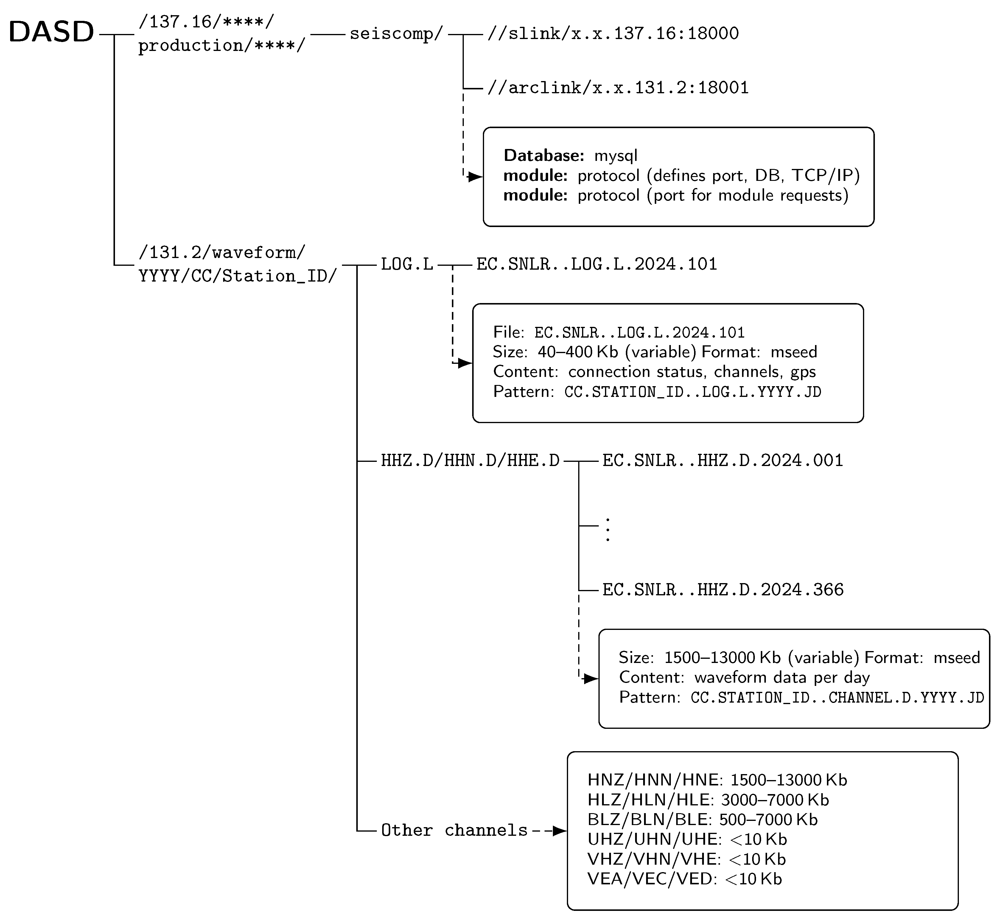
To automate recovery, the artifact needs a mapping between the station-side data source (remote storage/buffer) and the acquisition archive structure at the monitoring center. The mapping connects station identifiers, channels, calendar time ranges, and destination directories. For completeness, the directory tree view of a representative acquisition storage structure and the full CHANNEL/LOG mapping tables are provided in Appendix A and Appendix B, respectively.

PRT does not perform scientific format conversion (e.g., it does not transform waveforms into alternative analysis formats). Instead, it aligns packaging granularity with the acquisition archive by selecting the station-side files that cover missing time ranges and, when needed, reassembling the recovered waveform payload into daily archive units that follow the center-side naming and partitioning rules (year + Julian day). Importantly, this operation preserves the original waveform samples; only file packaging is aligned with the acquisition archive requirements.

Gap identification is driven by archive continuity at the monitoring center. Missing daily entries and abnormal file sizes provide a first-order discontinuity signal, while embedded timestamps allow bounding gap start/end times at sub-day resolution for reporting and visualization. Given a calendar time window, the mapping supports an operational workflow: (i) build a time-bounded query in the station-side store using calendar timestamps (YYYYMMDDhhmmss); (ii) retrieve matching station-side entries for that interval; and (iii) reassemble daily archive units indexed by year and Julian day (YYYY.JD) for ingestion at the center. The full pseudocode is provided in Procedure 1 and Appendix C (Algorithm A1).

In practice, a calendar-based time range may span multiple Julian days when its start and end timestamps cross a day boundary. For example, a query spanning from EC-ILLI_4-S-20240408000000 to EC-ILLI_4-S-20240408235959 covers two consecutive calendar days (8 April 2024 and 9 April 2024), which correspond to Julian days 099 and 100. Therefore, the associated content is distributed across daily files such as EC.ILLI..HHZ.D.2024.099 and EC.ILLI..HHZ.D.2024.100. Detailed step-by-step examples are provided in Appendix C.

Procedure 1 End-to-end recovery workflow for addressing recovered waveforms into the acquisition system.

Input: Station key, date range $\mathcal{D}$, mapping type $T\in \{\mathsf{CHANNEL},\mathsf{LOG}\}$, acquisition destination root

Output: Recovered daily archive files are injected into the acquisition storage with duplication checks

1: Identify candidate gaps using continuity indicators (JD identifiers, timestamps, file sizes, or missing sequence numbers).

2: Select candidate file class: prioritize recoverable data; ignore damaged/irrelevant entries when possible.

3: Recover/reassemble daily archive files from station-side entries by calling Algorithm A1 (Appendix C).

4: Validate outputs: basic integrity checks, expected naming pattern, and overlap/duplication checks against existing archive days.

5: Copy or inject recovered daily files into acquisition storage, update indices if required, and log the recovery action.

5. Proposed Recovery Artifact

5.1. Artifact Overview, Goals, and Deployment

We propose the Python Recovery Tool (PRT), a lightweight command-line Python script for post-outage backfilling in seismic/volcanic monitoring deployments. PRT runs on a standard operator laptop and connects to two endpoints: (i) the acquisition center and (ii) remote station hosts. After reconnection, the link goes up, PRT retrieves buffered records from the station-side store, extracts the useful waveform payload, and reassembles daily archive units compatible with the acquisition center (year–Julian day partitioning), delivering them with minimal operational disruption.

PRT follows three design goals:

• G1: Recover original data. Retrieve buffered records and backfill missing intervals at the acquisition center.
• G2: Low bandwidth. Reduce channel usage by avoiding redundant encapsulation and by sending only the required payload.
• G3: Retrofit. Work with legacy equipment and existing acquisition storage without hardware replacement.

Station-side requirements. PRT does not require a dedicated agent at the station. The only station-side requirement is SSH, FTP, HTTP, or SFTP access to the buffer directories, depending on the station and standard command-line tools for listing and transferring files.

Center-side interface. PRT delivers recovered daily waveform archives using the same naming and partitioning conventions expected by the acquisition environment, so the monitoring center can ingest them without changes to the existing data acquisition system. To support safe repeated executions, PRT produces a per-run report that records (i) successfully transferred file identifiers, (ii) missing expected files, and (iii) files rejected by integrity screening (e.g., abnormal size). In subsequent runs, these identifiers are used for best-effort duplicate avoidance and to skip entries previously flagged as corrupted.

5.2. Workflow, Gap Handling, and Efficiency

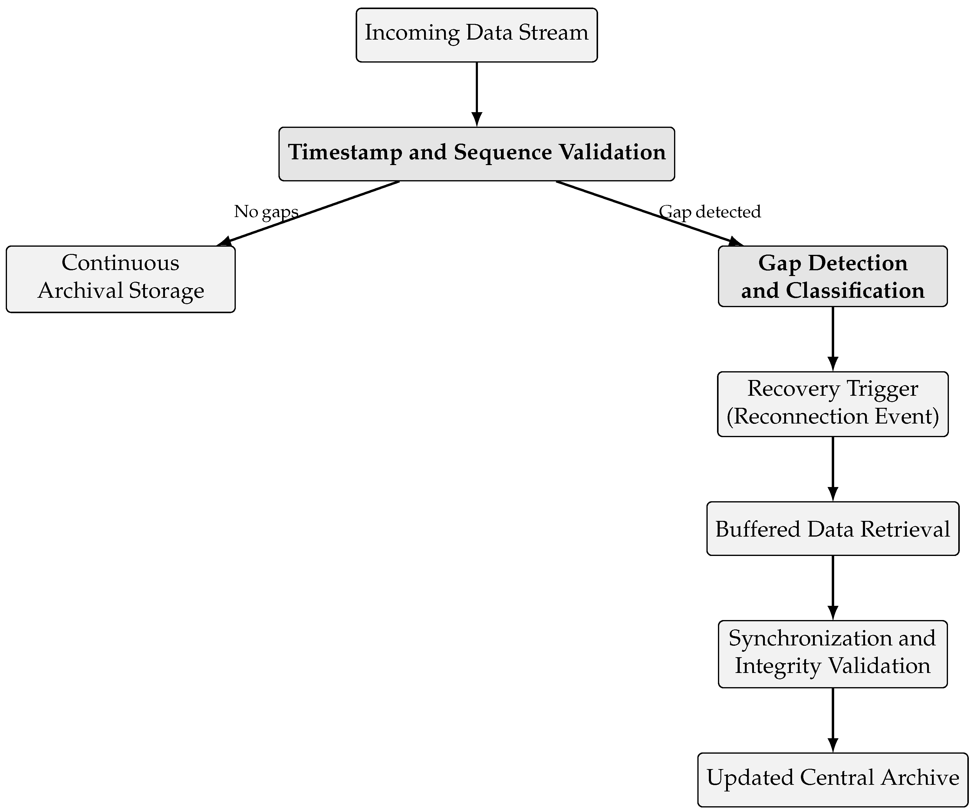
Figure 1 summarizes the workflow of the proposed system.

The workflow illustrated in Figure 1 describes how incoming data streams are first subjected to timestamp and sequence validation to ensure temporal continuity. When no discontinuities are detected, data are immediately written to the archive through a continuous storage process. If a temporal gap is identified, the system classifies the discontinuity and activates a recovery mechanism upon reconnection. During this phase, buffered waveform segments stored at the station or datalogger level are retrieved and reintegrated into the archive. A synchronization and integrity validation step ensures that recovered records are chronologically consistent and free of duplication before updating the central archive. This design minimizes data loss while maintaining operational efficiency and archive consistency.

After reconnection, PRT executes the steps below:

• Session trigger. Confirm that the station is reachable (light probe) and start a recovery session after a successful connection.
• Gap detection. Identify missing time windows by discontinuities/indices in the archive organization (year + Julian day partitions and time coverage). When station-side indices exist (ordered records or timestamps in the buffer), they are used to bound the recovery window.
• Candidate selection and mapping. Locate candidate records in the station store using mapping parameters and time-bounded queries. The mapping logic follows Algorithm A1 (Appendix C).
• Gap classification and filtering. Once connectivity is established, the filtering stage queries only the directory specified by the descriptor file (i.e., the folder where the waveform files actually reside), and does not traverse other paths. PRT then performs a two-step file-level screening before attempting recovery: (i) existence check: it compares the list of expected waveform filenames (derived from the descriptors) against the files present in that directory, immediately flagging any missing entries and reporting their identifiers; (ii) integrity check: for the remaining files, it validates basic consistency using a pre-defined acceptable range of file_size (and, when available, number_of_records with fixed record_length in our exports). Files with file_size outside the specified bounds (e.g., zero-sized or abnormally large) are marked as corrupted/malformed and rejected.
• Payload extraction and reassembling. PRT does not perform scientific format conversion: it preserves the original record format produced by each datalogger (as listed in the sensor/datalogger inventory table) and selects only the file types worth recovering. In practice, this step filters the station-side dataset to waveform files needed to fill acquisition gaps, while discarding non-essential products such as State-of-Health (SoH), internal monitoring components, recovery/debug artifacts, logs (e.g., sdata, md5), and low-rate preview streams (e.g., 1 Hz quick-look traces). The selected waveform files are then reassembled into standard daily archive units compatible with the acquisition center’s naming and partitioning rules (year + Julian day partitioning) and ready for ingestion. Any downstream format conversion, when required, is performed by the acquisition environment or by external operational tools integrated into the management/visualization workflow (e.g., those associated with the platforms listed in Table 1), not by PRT itself.
• Transfer and validation. Recovered daily waveform archives are transferred to the acquisition center and enqueued into the normal ingestion path. The center is able to process late-arriving data (out-of-order in time) and retroactively fill the corresponding gaps without disrupting ongoing acquisition. After transfer, PRT validates successful insertion, updates its local recovery state, and records delivered file identifiers to prevent re-sending duplicates in subsequent recovery cycles. The end-to-end injection workflow follows Procedure 1 in Section 4.

It is worth noting that monitoring stations often store or transmit waveform data inside proprietary record structures. PRT reduces overhead by extracting only the files required to reassemble the missing waveform segments at the center. At a high level, PRT keeps (i) timing information needed to place samples on the correct time axis; (ii) stream identifiers (station/channel codes); and (iii) the encoded sample payload.

PRT ignores redundant transport wrappers, repeated metadata that can be derived from configuration/mapping tables, and any padding or auxiliary fields that do not contribute to waveform reconstruction. This design reduces transmitted bytes and shortens recovery time under constrained throughput.

For logging purposes, each execution produces a timestamped, plain-text run report, organized per station (IP) and per requested day/time window. The report contains the following fields: (i) run identifier and execution timestamp(s); (ii) station identifier (e.g., IP and/or station code); (iii) target date and partitioning information (e.g., year and Julian day) and, when applicable, the requested time window; (iv) the list of expected waveform filenames generated from the descriptor information; (v) the list of successfully recovered/downloaded files; (vi) the list of missing files (expected but not found), including their derived station/channel/date identifiers; (vii) the list of corrupted/malformed files (found but rejected by size-range validation). The station, channel, and date fields can be reported explicitly because they are encoded in the waveform filename.

6. Evaluation Methodology

This section explains how we evaluated the proposed software tool. We focus on operational recovery after communication outages using evidence available in routine monitoring operations. In particular, we evaluate (i) archive-level data availability before recovery, (ii) recovery efficiency under the dump baseline, and (iii) recovery time under constrained link capacity.

6.1. Operational Evidence and Event-Driven Observation Windows

The evaluation uses operational data from the seismic and volcanic monitoring network of the Instituto Geofísico de la Escuela Politécnica Nacional (IG-EPN), Ecuador. Stations are deployed in remote environments and rely on heterogeneous communication links. To mitigate intermittent connectivity, stations maintain local buffering that can store waveform data for several days (depending on channel configuration and storage capacity). This operational setup makes post-outage backfilling feasible and motivates the use of an external recovery tool.

To show the relevance of our proposed tool, we analyze short event-driven windows centered on significant seismic episodes. These episodes are the most demanding periods for the data acquisition system: multiple stations and channels produce sustained waveform streams, and the acquisition center may experience bursts of arrivals and temporary ingestion lag. As a result, even when stations successfully buffer the data, the center-side archive may exhibit persistent discontinuities that require manual reprocessing.

6.1.1. Operational Data Sources

Our analysis relies on evidence available at the acquisition/archive layer and on station-side file listings. The primary sources are waveform files stored in predefined raw-data and archive directories at the monitoring center. From these files, we extract: timestamps, file sequence, file size, and extensions, which together allow reconstruction of temporal continuity under the same partitioning scheme used by the acquisition system.

When needed for interpretation (but not as a requirement for quantification), we also consult auxiliary indicators such as link monitoring logs and acquisition status messages. This design choice reflects operational reality: outages in monitoring signals may occur without explicit link-down notifications, whereas the archive provides the definitive evidence of what is missing at the center.

6.1.2. Window Definition and Archive-Level Discontinuities

For each selected event, we define a short time window W (typically a few consecutive days) that spans the episode and its immediate context. In this study, all cases use a fixed observation window of $W=96$ h (four consecutive days), defined in UTC from 00:00:00 on the first day to 23:59:59 on the fourth day. Within W, we treat a gap as an archive-level discontinuity, i.e., a missing time interval in the center-side waveform archive. Gaps are identified by continuity checks on the organization of the archived waveform: daily partitioning (Julian day), filename conventions, and embedded timestamps allow the detection of missing segments with minute-level resolution [37].

Importantly, we do not attempt to model the underlying cause separately (e.g., RF outage vs. ingestion backlog). Instead, we evaluate recovery strictly from the archive perspective, because this is the information available to analysts during routine validation. This perspective directly aligns with PRT: after reconnection, the tool retrieves the missing buffered content from the station-side store and reassembles daily archive units that can be re-ingested by the acquisition center.

6.2. Evaluation Metrics

Our evaluation targets post-outage back-filling under constrained links in heterogeneous legacy monitoring deployments. Stations store not only target waveform streams but also auxiliary content (e.g., logs, calibration files, vendor-specific streams). In addition, recovery operates at file granularity, so back-filling a gap interval may require transferring full files that overlap the gap boundaries. To avoid ambiguity, we separate time availability metrics (coverage) from byte counters (traffic and baselines). For each station s, we analyze a fixed observation window W. Within W, we first report operational byte counters that describe station inventory, pre-recovery availability at the data center, and recovery traffic. We then derive time- and traffic-based metrics that quantify coverage, efficiency relative to a naive dump baseline, and the modeled recovery time under constrained capacity.

In this context, the transfer time depends on two fundamental factors. On the one hand, it depends linearly on the transmitted volume, since it is a file-oriented transfer (not continuous streaming). On the other hand, it depends inversely on the available effective throughput, which is limited by the bottleneck link [38]. This association more accurately reflects the behavior observed in shared-channel acquisition systems with concurrent traffic than direct or instantaneous measurements of the time required for file recovery (RTO).

6.2.1. ByteCounters (Station s, Window W)

We define the following:

• $B_{\mathrm{sta}}(s,W)$: station stored bytes for W, computed from the station inventory/listing. This includes waveform and non-waveform content and represents the volume that a naive full dump approach would retrieve if no file-level interpretation is performed.
• $B_{\mathrm{dc}}(s,W)$: bytes available at the data center for W before recovery, measured over the target waveform streams/components only. This value is reported for context (how much is already present), but it is not used as a denominator for efficiency metrics.
• $B_{\mathrm{tx}}(s,W)$: bytes transmitted by the recovery tool to backfill missing waveform coverage within W, obtained from application-level counters/tool logs.

It is important to note that there are no additive relations among these counters. In particular, $B_{\mathrm{sta}}(s,W)$ is not expected to equal $B_{\mathrm{dc}}(s,W)+B_{\mathrm{tx}}(s,W)$ because (i) $B_{\mathrm{sta}}$ includes auxiliary/non-target station content; and (ii) $B_{\mathrm{tx}}$ may over-fetch due to coarse file granularity and temporal overlap. All byte counters are measured in bytes and reported in MB for readability.

6.2.2. Time-Based Availability (Pre/Post Recovery)

Let $H_W$ denote the duration of W in hours (e.g., $H_W=96$ for four days). From the acquisition waveform timeline (UTC), we compute the total gap time as the sum of all missing intervals, denoted by $D_{\mathrm{gap}}(s,W)$ before recovery and $D_{\mathrm{gap}}^{\prime }(s,W)$ after backfilling. We report:

$$A_{\mathrm{pre}}(s,W)=\left(1-{\displaystyle \frac{D_{\mathrm{gap}}(s,W)}{H_W}}\right)\times 100,$$

(1)

$$A_{\mathrm{post}}(s,W)=\left(1-{\displaystyle \frac{D_{\mathrm{gap}}^{\prime }(s,W)}{H_W}}\right)\times 100.$$

(2)

Here, D denotes gap duration and A denotes time availability over the fixed window W.

6.2.3. Recovery Traffic Relative to a Naive Full Dump Baseline

To quantify the traffic benefit of selective recovery, we use the dump baseline as the naive strategy that transfers the entire station-side volume in bytes for the window. The proposed tool is evaluated by its transmitted volume relative to that baseline:

$${\eta }_{\mathrm{dump}}(s,W)={\displaystyle \frac{B_{\mathrm{tx}}(s,W)}{B_{\mathrm{sta}}(s,W)}}.$$

(3)

where $B_{\mathrm{tx}}(s,W)$ is the transmitted byte volume during recovery and $B_{\mathrm{sta}}(s,W)$ is the total station-side byte volume stored during W.

For better interpretation, we report the corresponding traffic reduction percentage:

$$S_{\mathrm{dump}}(s,W)=\left(1-{\eta }_{\mathrm{dump}}(s,W)\right)\times 100.$$

(4)

Because recovery is file-based, the tool may need to transmit files that extend beyond the exact missing intervals. Therefore, $B_{\mathrm{tx}}(s,W)$ depends on the missing interval and the underlying file granularity/packaging.

6.2.4. Modeled Recovery Time Under Constrained Effective Capacity

To translate the transmitted recovery volume into an operational impact, we model the recovery time as follows:

$$T_{\mathrm{rec}}(s,W)={\displaystyle \frac{8·B_{\mathrm{tx}}(s,W)}{C_{\mathrm{eff}}\left(s\right)}},$$

(5)

$$T_{\mathrm{cur}}(s,W)={\displaystyle \frac{8·B_{\mathrm{sta}}(s,W)}{C_{\mathrm{eff}}\left(s\right)}},$$

(6)

where $C_{\mathrm{eff}}\left(s\right)$ denotes the effective recovery throughput (bits/s) available on the bottleneck path between the station and the data center during the recovery phase. We define the following:

$$C_{\mathrm{eff}}\left(s\right)=max\left(0,C_{max}\left(s\right)-C_{\mathrm{res}}\left(s\right)\right),$$

(7)

with $C_{max}\left(s\right)$ bottleneck link capacity and $C_{\mathrm{res}}\left(s\right)$ conservative reserved rate to protect routine telemetry and operational traffic. In our evaluation, $C_{max}\left(s\right)$ is taken from the link configuration or from operational measurements along the station–center path (e.g., last-mile radio, microwave hop, or fiber segment), and corresponds to the minimum configured/measured capacity across the hops. To preserve routine traffic, we set a conservative reserved rate

$$C_{\mathrm{res}}\left(s\right)=\kappa R_{\mathrm{avg}}\left(s\right),$$

(8)

with $\kappa =3$ in this study. This rule-of-thumb reserves headroom for short-term telemetry peaks under normal operation so that recovery does not starve routine flows. Since $T_{\mathrm{rec}}$ scales inversely with $C_{\mathrm{eff}}=C_{max}-C_{\mathrm{res}}$, increasing $\kappa$ yields a more conservative (longer) recovery-time estimate, while a smaller $\kappa$ yields a more aggressive estimate.

Within this framework, the term $Cres$ is adopted as a practical engineering criterion to include the effects of acquisition system degradation during the data recovery phase. $Cres$ is not an arbitrary value but is aligned with recent theoretical and empirical evidence related to delay, resilience, and traffic variability in distributed networks. Additionally, the parameter $\kappa =3$ represents a conservative margin widely used in telecommunications for overprovisioning and practical approximations. Its adoption is based on queuing theory and the stochastic (and even chaotic) nature of data traffic [38,39].

Accordingly, $T_{\mathrm{rec}}$ provides a conservative estimate of the time required to backfill the transmitted volume $B_{\mathrm{tx}}$ under constrained links. In contrast, $T_{\mathrm{cur}}$ corresponds to the naive download time estimate. If $C_{\mathrm{eff}}\left(s\right)=0$, recovery is not feasible under the reserved margin, and recovery is deferred until capacity becomes available or the reserved margin is adjusted.

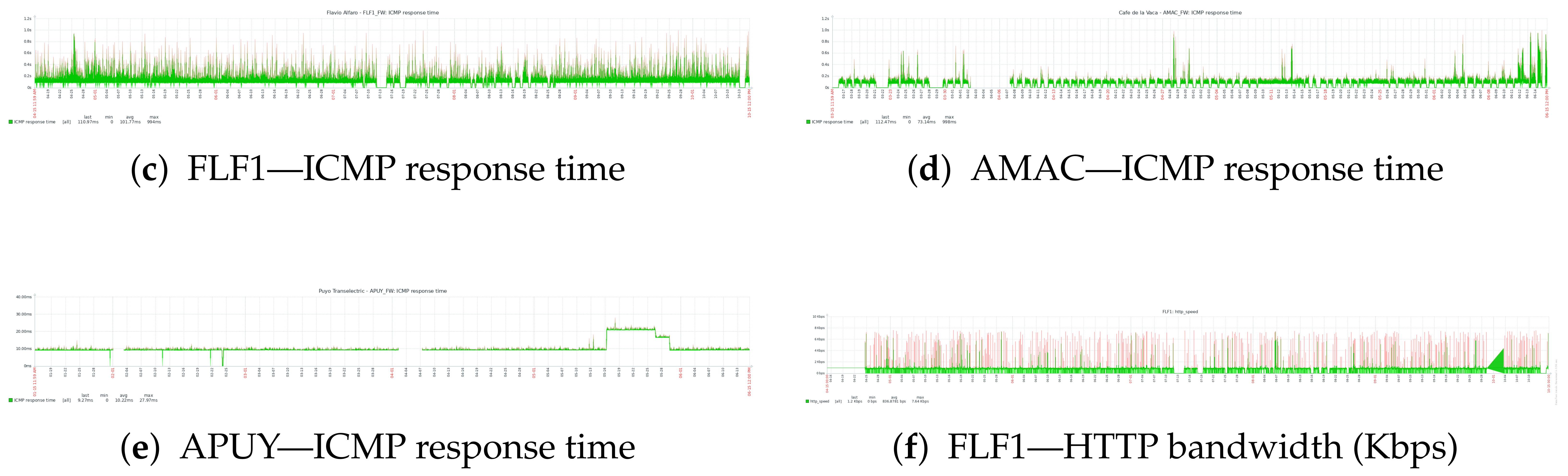
These charts, spanning several months, illustrate the variability in response time and data throughput, underscoring the need to estimate an average rather than rely on a precise, real-time measurement of channel capacity. The much longer time periods (months) support the validity of $Cres$ and k used in this study with shorter periods (days), as the Figure 2 summarize the variability mentioned above.

7. Results

This section reports results for five operational recovery cases selected around significant seismic episodes, where acquisition backlogs and intermittent connectivity can yield persistent archive discontinuities.

Following the time- and byte-based evaluation defined in Section 6.2, each case is characterized by the following: (i) pre- and post-recovery time availability ($A_{\mathrm{pre}}$, $A_{\mathrm{post}}$) derived from the waveform timeline; (ii) the station inventory volume used as a naive dump baseline ($B_{\mathrm{sta}}$); (iii) the data-center pre-recovery volume ($B_{\mathrm{dc}}$) reported for context; (iv) the transmitted recovery volume ($B_{\mathrm{tx}}$); and (v) the resulting dump-relative traffic reduction ($S_{\mathrm{dump}}$) and modeled recovery time ($T_{\mathrm{rec}}$) under constrained effective throughput $C_{\mathrm{eff}}$. To keep the presentation compact while preserving auditability, we summarize the time availability in

Table 2. Pre-recovery status for five operational cases (gap duration and time availability).

Case	Station	Window (UTC)	Dgap	Apre (%)	Bdc (MB)
C1	SAG1	2025-06-03 … 2025-06-06	01 d 09 h 24 m	65.21	148.91
C2	ESM1	2025-02-21 … 2025-02-24	02 d 12 h 35 m	36.90	64.13
C3	FLF1	2025-07-19 … 2025-07-22	G1:01 d 09 h 50 m	61.85	43.14
			G2:00 d 01 h 07 m
			G3:00 d 00 h 44 m
			G4:00 d 00 h 56 m
C4	AMAC	2025-08-15 … 2025-08-18	G1:00 d 02 h 24 m	76.51	103.64
			G2:00 d 01 h 40 m
			G3:00 d 08 h 47 m
			G4:00 d 08 h 01 m
			G5:00 d 04 h 05 m
C5	APUY	2025-02-23 … 2025-02-26	00 d 05 h 17 m	94.50	115.78

and the recovery effort in

Table 3. Recovery effort and outcome metrics for five operational cases.

Case	Station	Bsta (MB)	Btx (MB)	Cmax (kbps)	Ravg (kbps)	Sdump (%)	Trec (min)
C1	SAG1	238.08	84.32	884	16.40	64.58	13.47
C2	ESM1	167.60	66.60	115	12.35	60.26	113.92
C3	FLF1	205.92	196.80	154	9.20	4.43	207.59
C4	AMAC	186.24	43.75	154	20.30	76.51	62.66
C5	APUY	163.20	10.20	2000	90.60	93.75	0.79

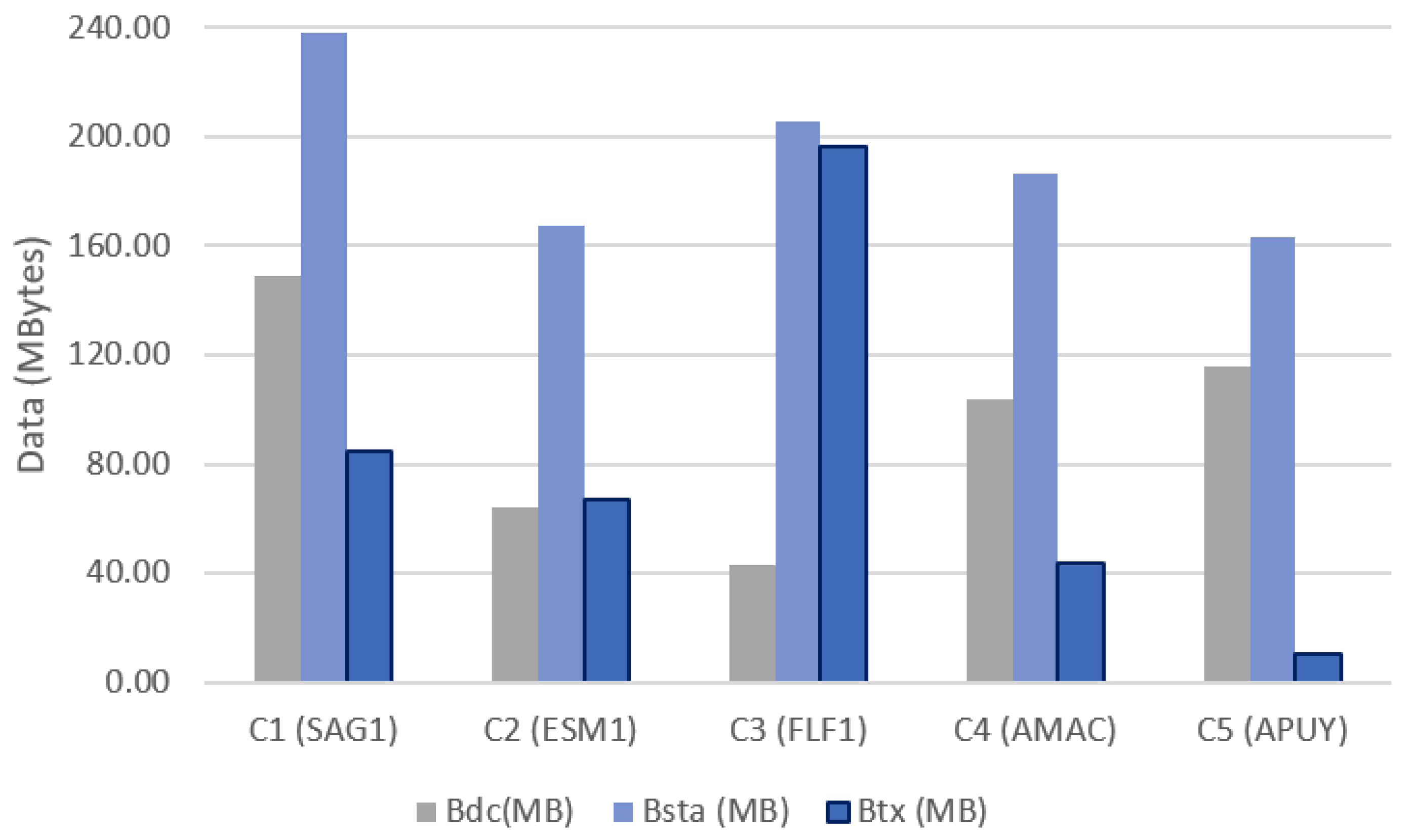
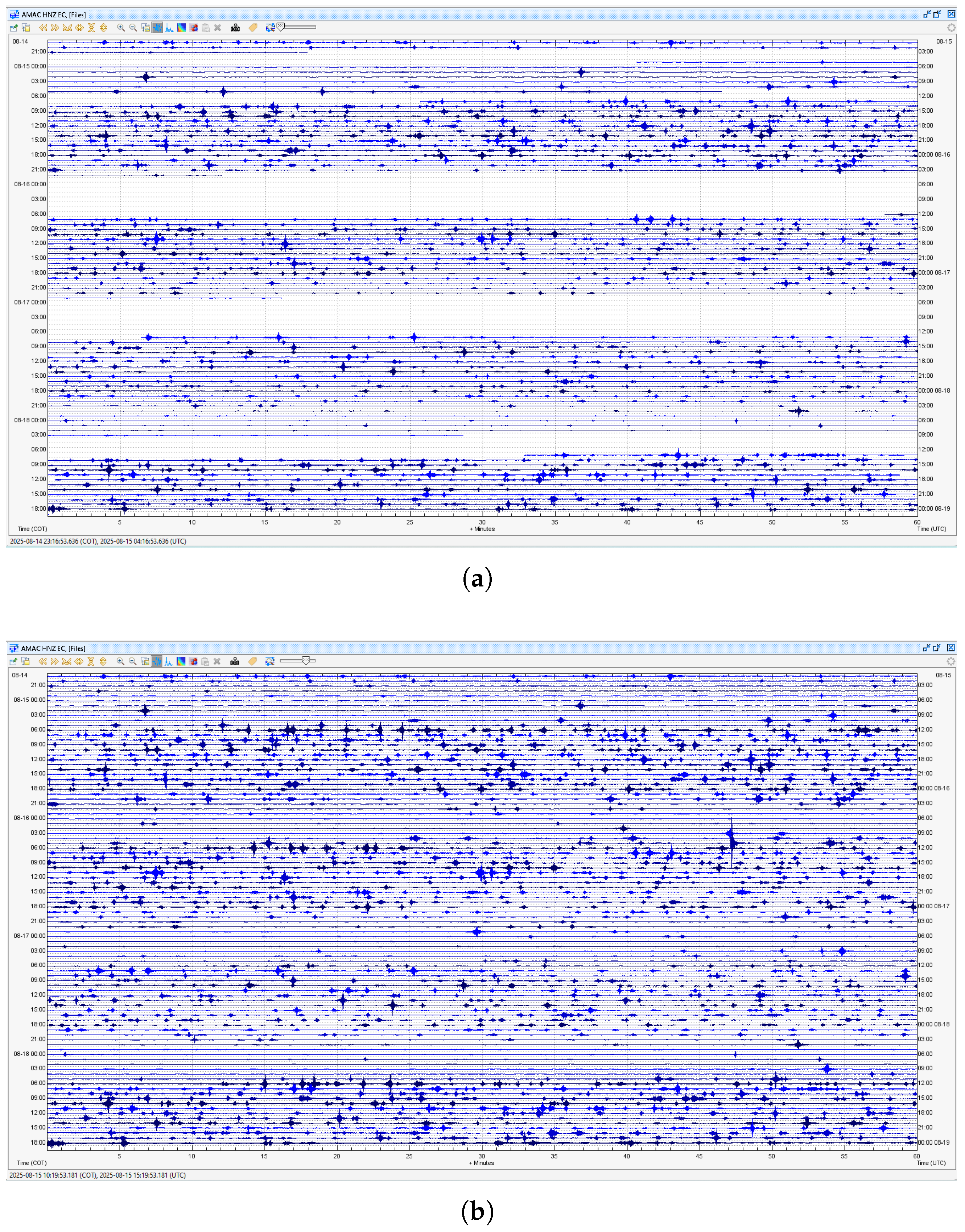
. A long single gap overlapping an event are shown in Figure 3, together with its corresponding recovery. These results are further complemented by three figures: a cross-case byte-volume comparison Figure 4, a recovery-time comparison Figure 5, and a representative before/after waveform continuity visualization Figure 6.

Together, these outputs connect the archive deficit observed at the monitoring center with the recovery effort required over constrained links, providing quantitative and visual evidence of post-outage backfilling performance.

7.1. Pre-Recovery Status: Gaps and Time Availability

Table 2 summarizes the pre-recovery status of the five operational cases over the observation window W, selected around relevant seismic episodes (M > 3) recorded in Ecuador during 2025. All windows span $W=96$ h in UTC (00:00:00 to 23:59:59 over four consecutive days). All stations belong to the IG-EPN seismic–volcanic monitoring network and operate with real-time data transmission capabilities over heterogeneous links [40]. For each case, we quantify (i) the total missing time at the acquisition center, $D_{\mathrm{gap}}$, and (ii) the corresponding pre-recovery time availability $A_{\mathrm{pre}}$ (Equation (1)), derived from the waveform timeline under the same archive partitioning used by the acquisition system. We also report $B_{\mathrm{dc}}$ as contextual evidence of how much target waveform data was already present at the monitoring center before any backfilling action.

The selected windows are centered on cataloged earthquakes that drive operator workload and subsequent forensic analysis. During these episodes, complete waveform time coverage is required for reliable event detection, phase picking, location, and magnitude estimation and, when available, multi-parameter correlation (e.g., seismic velocity channels combined with infrasound). Gaps in the archive can therefore impact both near-real-time assessment and later reprocessing. The five cases represent realistic conditions in which stations keep recording locally while the acquisition center exhibits discontinuities, either as a single dominant gap (continuous missing interval) or as fragmented discontinuities distributed over multiple days.

The cases cover two pre-recovery patterns. First, C1, C2, and C5 show a single dominant gap within W. Second, C3 and C4 exhibit multiple disjoint gaps (C3:G1–G4, C4:G1–G5) in the same 4-day window, revealing fragmented archive discontinuities that reduce time coverage even when no single outage dominates. Across the five cases, $A_{\mathrm{pre}}$ spans a wide range (from 36.90% to 94.50%), highlighting that archive completeness prior to recovery can vary substantially depending on station conditions and the operational stress induced by event-driven data bursts.

7.1.1. Case C1 (SAG1): Long Single Gap Overlapping an Event

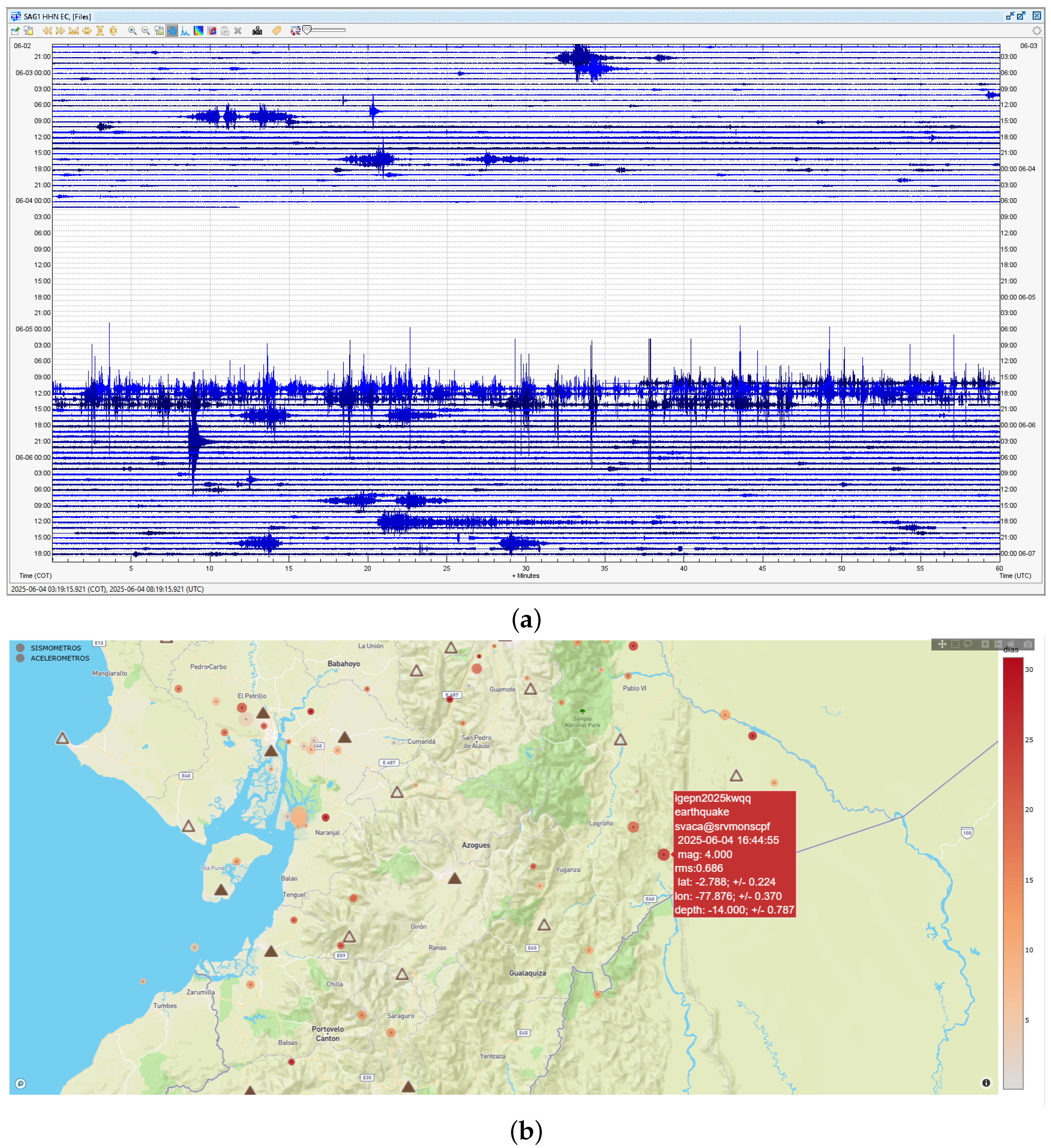
C1 (SAG1) presents a continuous but extensive gap of 01 d 09 h 24 m, resulting in $A_{\mathrm{pre}}=65.21\%$ (Table 2). Within this missing interval, a local event [41] of magnitude 4.0 MLv occurred on 2025-06-04 16:44:55 UTC, (Event Code: igepn2025kwqq) [42]. Figure 3a illustrates the pre-recovery waveform availability at SAG1 and visually identifies the start/end of the gap, while Figure 3b provides the associated event context. For this station, the primary target streams for continuity correspond to the three-component velocity channels (HHZ/HHN/HHE) and the infrasound channel (BDF), which are relevant for event analysis and multi-parameter correlation during the selected window.

Figure 3. (a) SAG1 station data availability and detected gap [42]. (b) Associated seismic event (M 4.0 MLv). Source: Seismic reports of IG-EPN, 2025, Event Code: igepn2025kwqq. (a) SAG1 Station (e.g., HHN), data range 20250603 to 20250606. Gap: 20250604 (06:11:00) to 20250605 (15:35:10) UTC. (b) Earthquake, magnitude 4.0 MLv, UTC 2025/06/04 16:44:55, depth 14.3 km.

Figure 3. (a) SAG1 station data availability and detected gap [42]. (b) Associated seismic event (M 4.0 MLv). Source: Seismic reports of IG-EPN, 2025, Event Code: igepn2025kwqq. (a) SAG1 Station (e.g., HHN), data range 20250603 to 20250606. Gap: 20250604 (06:11:00) to 20250605 (15:35:10) UTC. (b) Earthquake, magnitude 4.0 MLv, UTC 2025/06/04 16:44:55, depth 14.3 km.

7.1.2. Case C2 (ESM1): Very Low Pre-Recovery Availability over the Event Window

C2 (ESM1) exhibits the lowest time availability among the five cases ($A_{\mathrm{pre}}=36.90\%$), associated with a gap of 02 d 12 h 35 m over W. Such a deficit implies that more than half of the time window is missing at the acquisition center, which compromises event-driven reprocessing. This window includes a regional earthquake of magnitude 5.3 MLv on 2025-02-23 07:25:15 UTC (Event Code: igepn2025dtkg) [42], where completeness is relevant not only for detection/location but also for subsequent propagation and intensity analyses at different distances from the epicenter.

7.1.3. Case C3 (FLF1) and Case C4 (AMAC): Fragmented Discontinuities (Multiple Gaps)

C3 (FLF1) and C4 (AMAC) show multiple gap episodes within the same 4-day window (G1–G4, G1–G5 in Table 2). Rather than a single continuous missing interval, the archive presents segmented discontinuities that accumulate into substantial missing time (C3: $A_{\mathrm{pre}}=61.85\%$; C4: $A_{\mathrm{pre}}=76.51\%$). For C3, the analyzed window contains a coastal event of magnitude 4.4 MLv on 2025-07-20 21:06:29 UTC (Event Code: igepn2025odak) [42], for which incomplete time coverage can reduce the reliability of event-level review. For C4, the affected streams correspond to acceleration channels (HNZ/HNN/HNE), where continuity is important for engineering-oriented indicators and intensity-related studies. This analyzed window contains a significant event of magnitude 4.7 MLv on 2025-08-16 10:46:58 UTC (Event Code: igepn2025pzoo) [42] near the active Cotopaxi volcano. The station recorded the event locally; however, the acquisition archive at the monitoring center is incomplete due to multiple gaps, which account for 23.49% of missing waveform time within W.

7.1.4. Case C5 (APUY): High Availability with Residual Short Gaps

C5 (APUY) shows the highest pre-recovery availability ($A_{\mathrm{pre}}=94.50\%$) and the shortest gap duration (00 d 05 h 17 m) among the analyzed windows. This case emphasizes that even when overall connectivity is comparatively strong, residual archive discontinuities may still occur and remain visible at the center, thus motivating selective backfilling to achieve complete event windows. The station is also geographically close to the regional event referenced in C2, making its waveforms relevant for location refinement and post-event analyses (e.g., aftershock activity in the same source region).

The sample size (deterministic sampling) represented by the five operational cases has been dimensioned to ensure analytical validity in critical operational scenarios and does not aim for statistical representativeness based on random cases or the probability of occurrence of gaps in seismic–volcanic monitoring networks [43].

Commonly, from a seismological and real-time monitoring perspective, long periods of seismic activity may be characterized by a low or stable trend. However, when tectonic or volcanic activity increases, the volume of transmitted data increases, potentially leading to channel saturation. Furthermore, the physical network infrastructure can be affected by large-magnitude earthquakes or volcanic activity. Therefore, in this study, the sample size has focused on these episodes where a gap can be crucial for interpreting seismic or volcanic behavior, rather than analyzing extended periods (months or years) of low activity.

Each case was selected based on relevant seismic events with different discontinuity patterns, characterized by maximum load conditions on the acquisition and transmission system, with varying levels of availability and heterogeneity of links and data formats at the source.

This allows us to infer properties of the system’s behavior under limiting conditions, which is consistent with the approaches used in distributed systems and sensor networks. Furthermore, it enables the practical representation of stress tests on data traffic between monitoring points and the data center [39].

7.1.5. Consideration of “Non-Target” Content in Standard Transfers

In standard acquisition workflows, stations may also deliver auxiliary or low-priority products (e.g., state-of-health and monitoring channels) that are not required for waveform continuity in the target archive. In this study, Table 2 focuses strictly on the waveform time coverage deficit observed at the acquisition center prior to recovery. The recovery actions and their corresponding cost (file selection, station-side locations, transferred volume, and link-constrained recovery time) are quantified next in Section 7.2.

7.2. Recovery Effort: Transmitted Volume, Savings, and Recovery Time

Table 3 summarizes the recovery effort and the resulting performance indicators for the five cases. We use the station-side inventory volume $B_{\mathrm{sta}}$ as the baseline for a naive dump that would retrieve the full station dataset over the same window W. $B_{\mathrm{tx}}$ corresponds to the volume transmitted by PRT to backfill the missing waveform segments within W. $C_{max}$ is the bottleneck capacity (kbps) along the end-to-end path between the station and the acquisition center, while $R_{\mathrm{avg}}$ denotes the average bitrate generated by the station (kbps), estimated from medium-term operational counters. Efficiency is reported as the dump-relative traffic reduction $S_{\mathrm{dump}}$ (in %), which captures how much download volume is avoided by PRT compared to retrieving the full station dataset for the same window. The modeled recovery time $T_{\mathrm{rec}}$ is obtained using Equation (5) under the effective throughput $C_{\mathrm{eff}}$ and is expressed in minutes to improve interpretability. Finally, $A_{\mathrm{post}}$ (Equation (2)) captures the post-recovery time availability over the same evaluation window.

In addition, $D_{\mathrm{gap}}^{\prime }(s,W)$ is less than 1% for the five stations analyzed in Table 2 and Table 3.

While these aggregated metrics provide a compact view of recovery efficiency, they do not explicitly capture how missing time intervals are mapped to specific station-side resources. To complement the quantitative assessment, a case-level perspective is required to link observed archive deficits with the underlying file structures and storage locations at the station. The following subsection therefore details the operational recovery scope in terms of files and station-side directories involved in each case.

Case-Level Recovery Scope (Files and Station-Side Locations)

To make the recovery effort tangible, we briefly summarize how archive deficits map to station-side buffered content in each case. PRT performs time-bounded retrieval constrained to the waveform directories specified by station descriptors, and applies file-level screening (existence and integrity checks) before transfer:

• C1 (SAG1): The acquisition archive contains incomplete daily waveform files for the event window (e.g., EC.SAG1..HHZ.D.2025.154–157, similarly for HHN/HHE/BDF). PRT maps the missing span to station-side buffered labels in the data directory (e.g., EC-SAG1_4-20250604000000 to EC-SAG1_4-20250605235959), targeting the three-component velocity streams (HHZ/HHN/HHE) and the infrasound stream (BDF).
• C2 (ESM1): PRT identifies missing and incomplete daily files across multiple waveform channels (HH* and HN* families), including missing daily identifiers (e.g., ...2025.054) and abnormally small files in adjacent days. The station-side search is constrained to the year/day tree in the vendor buffer layout (e.g., ../2025/053/*Serie*/1/... to ../2025/055/*Serie*/1/...), limiting traversal to the waveform directory specified by descriptors.
• C3 (FLF1): Multiple disjoint gaps within the same 4-day window translate into several time-bounded retrieval spans. PRT resolves the affected daily waveforms (e.g., EC.FLF1..HHZ.D.2025.199–202) and maps them to station-side buffered labels under /data/ for the corresponding date ranges.
• C4 (AMAC): Similar to C3, recovery spans multiple disjoint gaps and requires repeated time-bounded selection in the station buffer. PRT identifies incomplete files (e.g., EC.AMAC..HNZ.D.2025.227–230) and maps the range of names of buffered files to be recovered in the station (e.g., ../2025227/*Serie*/1/010000000_xxxxxxxx to ../2025230/*Serie*/1/230000000_xxxxxxxx).
• C5 (APUY): Despite high pre-recovery availability, PRT detects a localized discontinuity in a specific stream (e.g., EC.APUY..HNZ.D.2025.055) and maps it to a small set of buffered files in the station layout (e.g., ../202502_APUY/202502240800.gcf to ../202502_APUY/202502241400.gcf).

Table 3 shows that $S_{\mathrm{dump}}$ varies substantially across stations, reflecting the extent to which selective backfilling can avoid bulk station retrieval under heterogeneous packaging and connectivity constraints. Importantly, $T_{\mathrm{rec}}$ is not determined by volume alone: cases with comparable transmitted volumes may yield very different recovery times because effective throughput depends on the bottleneck capacity along the multi-hop path and the reserved margin required for routine traffic.

7.3. Cross-Case Comparison of Byte Volumes and Efficiency

Figure 4 complements the tables by providing a compact cross-case view of (i) the naive dump baseline volume ($B_{\mathrm{sta}}$), (ii) the pre-recovery data-center volume ($B_{\mathrm{dc}}$), and (iii) the transmitted recovery volume ($B_{\mathrm{tx}}$). This visualization makes the disparity between naive bulk retrieval and selective backfilling visually comparable across cases.

Figure 4. Cross-case volume and recovery effort comparison. $B_{\mathrm{sta}}$ (station inventory dump baseline), $B_{\mathrm{dc}}$ (pre-recovery at center, contextual), and $B_{\mathrm{tx}}$ (tool transmitted volume).

Figure 4. Cross-case volume and recovery effort comparison. $B_{\mathrm{sta}}$ (station inventory dump baseline), $B_{\mathrm{dc}}$ (pre-recovery at center, contextual), and $B_{\mathrm{tx}}$ (tool transmitted volume).

Across cases, a lower $A_{\mathrm{pre}}$ indicates larger time coverage deficits prior to recovery. Lower $B_{\mathrm{tx}}$ relative to $B_{\mathrm{sta}}$ indicates improved efficiency under the dump baseline, summarized by $S_{\mathrm{dump}}$.

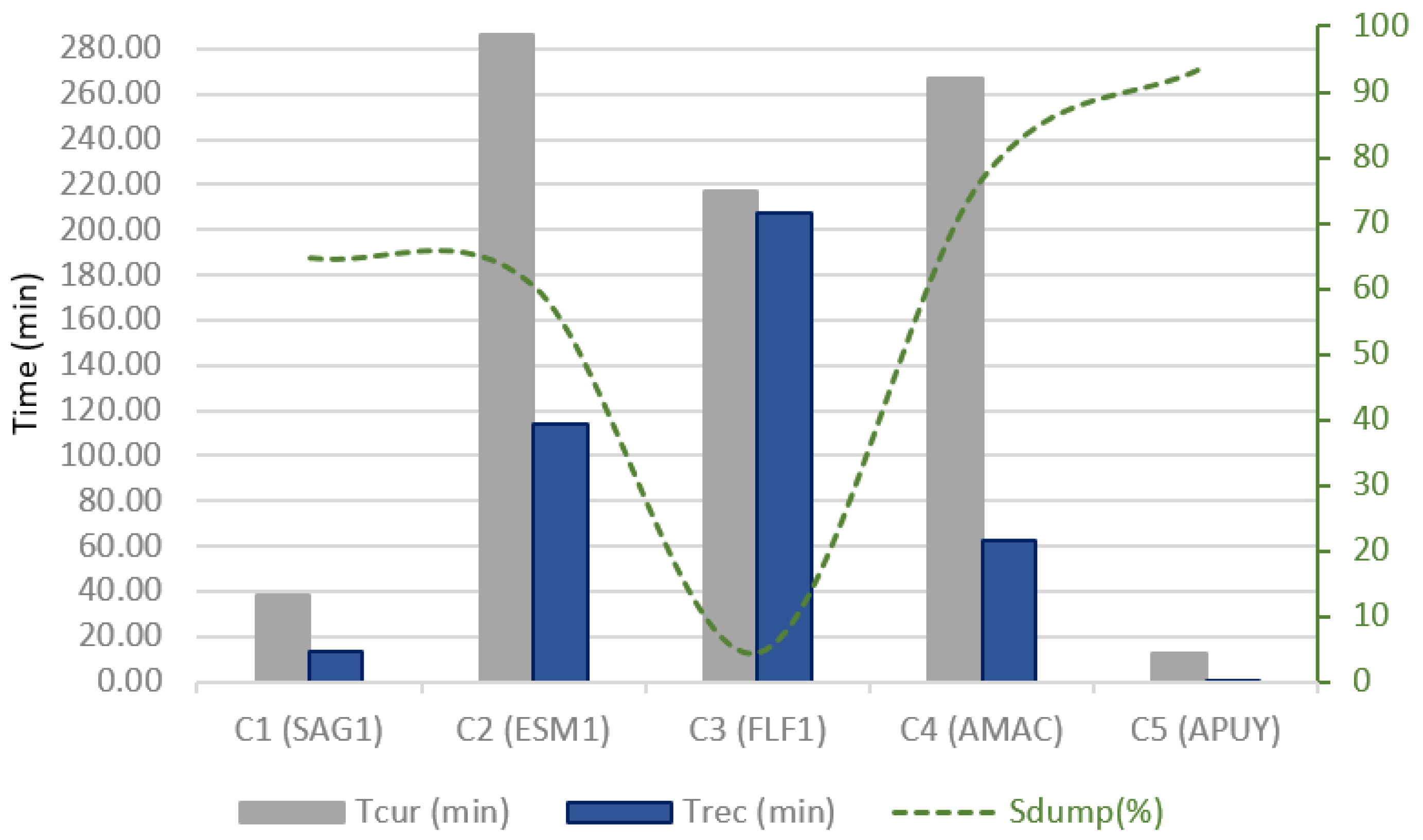
  While Figure 5 shows that the transmitted recovery volumes $B_{\mathrm{tx}}$ can be comparable across some cases, the time required to complete recovery may differ substantially once link heterogeneity is considered. This is because $T_{\mathrm{rec}}$ depends not only on the recovered volume but also on the effective throughput along the end-to-end path, which varies across stations due to different access technologies (e.g., satellite, microwave, last-mile radio, or fiber segments).

Figure 5. Modeled recovery time comparison under constrained effective capacity.

Figure 5. Modeled recovery time comparison under constrained effective capacity.

The bars show, for each case, the modeled time for the naive dump baseline (computed using $B_{\mathrm{sta}}$) versus the modeled PRT recovery time (computed using $B_{\mathrm{tx}}$), both under the same station-specific $C_{\mathrm{eff}}$. Although transmitted volumes may appear comparable in Figure 4, recovery times vary markedly across cases due to heterogeneous link capacities and operational constraints.

PRT achieves the largest traffic reductions when selective retrieval can avoid bulk transfers (e.g., C2 and C5), whereas efficiency is limited when the recovery requires transmitting a volume close to the station inventory (C3). Across the five cases, $S_{\mathrm{dump}}$ ranges from 4.43% to 93.75%, highlighting that the achievable savings depend on both archive deficits and station-side packaging constraints.

7.4. Waveform Continuity Before/After Recovery

To provide operational evidence, we visualize waveform continuity over time, highlighting the detected gap and the restored archive. Figure 6 shows a representative case (C4) with two panels: before recovery and after recovery. This figure is included for visual clarity rather than numeric comparison.

Figure 6. Waveform continuity visualization for a representative case (C4). (a) Acquisition waveform timeline before recovery, showing the gap(s) over W. AMAC Station, data range 20250815 to 20250818. GAP1: 20250815 (02:17:10) to 20250815 (04:40:34) UTC. GAP2: 20250815 (10:46:27) to 20250815 (12:25:41) UTC. GAP3: 20250816 (03:11:56) to 20250816 (11:57:44) UTC. GAP4: 20250817 (04:16:04) to 20250817 (12:06:27) UTC. GAP5: 20250816 (03:28:36) to 20250818 (12:32:52) UTC. (b) Timeline after recovery, showing restored continuity (ideally $D_{\mathrm{gap}}^{\prime }\le 1\%$). Data adapted from IG-EPN [42] (Event Code: igepn2025pzoo). Source: Seismic reports of IG-EPN, 2025. Earthquake, magnitude 4.7 MLv, UTC 2025/08/16 10:46:58, depth 8.3 km.

Figure 6. Waveform continuity visualization for a representative case (C4). (a) Acquisition waveform timeline before recovery, showing the gap(s) over W. AMAC Station, data range 20250815 to 20250818. GAP1: 20250815 (02:17:10) to 20250815 (04:40:34) UTC. GAP2: 20250815 (10:46:27) to 20250815 (12:25:41) UTC. GAP3: 20250816 (03:11:56) to 20250816 (11:57:44) UTC. GAP4: 20250817 (04:16:04) to 20250817 (12:06:27) UTC. GAP5: 20250816 (03:28:36) to 20250818 (12:32:52) UTC. (b) Timeline after recovery, showing restored continuity (ideally $D_{\mathrm{gap}}^{\prime }\le 1\%$). Data adapted from IG-EPN [42] (Event Code: igepn2025pzoo). Source: Seismic reports of IG-EPN, 2025. Earthquake, magnitude 4.7 MLv, UTC 2025/08/16 10:46:58, depth 8.3 km.

In summary, our results show that the recovery artifact restores waveform continuity after reconnection while reducing recovery traffic relative to a naive bulk station retrieval baseline. Under constrained throughput, the reduction in transmitted volume directly translates into shorter modeled recovery time.

Our evaluation relies on operational archive evidence and application-level byte counters. Recovery time is modeled under a conservative effective throughput $C_{\mathrm{eff}}$ and does not capture short-term rate fluctuations. Nevertheless, this methodology is appropriate for field-based validation in legacy deployments where controlled experiments are impractical.

8. Conclusions

We presented the Python Recovery Tool (PRT), a lightweight command-line artifact for post-outage waveform gap recovery in seismic–volcanic monitoring deployments, designed as a retrofit solution that does not require station-side agents or hardware upgrades. PRT leverages station-side buffering and performs time-aware, file-granular retrieval to backfill archive discontinuities at the monitoring center with minimal operational disruption.

A key contribution of this work is an archive-centric evaluation that uses the data-center archive as ground truth for what is missing, avoiding reliance on vendor-specific telemetry logs that may be incomplete in heterogeneous deployments.

Selective backfilling allows you to restore the continuity of a data file after an outage by focusing only on the missing segments instead of retransmitting the entire historical data volume. This targeted approach avoids unnecessary duplication and optimizes bandwidth usage, as recovery is strictly limited to the missing or incomplete segments.

Across five event-driven cases, the reported dump-relative traffic reduction spans 4.43–93.75%, and the modeled catch-up time ranges from 0.79 to 207.59 min under station-specific bottleneck capacities.

The proposed solution showed consistent usefulness across the interruption patterns represented by the selected stress-oriented cases. Although the sample size is limited, the purposeful selection of demanding operational episodes provides evidence that the recovery workflow remains effective under high-load conditions relevant to real monitoring practice. Broader long-term validation across extended operational periods remains part of future work.

Compared to naive bulk dump strategies, this technique substantially reduces recovery traffic. As a result, the post-outage process becomes viable even on last-mile links with limited capacity, where preserving routine operational telemetry and ensuring the continuity of real-time data flow are essential.

This work demonstrated that the PRT model implements a practical verification workflow aimed at improving the availability and consistency of recovered information in operational seismic monitoring environments. In its current form, the workflow combines file existence checks, expected size-range validation, duplicate avoidance, and temporal continuity verification at the data center to detect losses, interruptions, and inconsistencies during recovery. Furthermore, preserving the original datalogger format and validating waveforms through visual inspection (drum plots) allowed verification of content integrity from a seismological perspective, helping retain critical parameters such as sampling frequency, number of channels, and waveform structure. These results establish a scalable foundation for future developments, including checksum-based integrity verification, more explicit structural header validation mechanisms, and automated metadata validation through integration with specialized databases (e.g., gempa, FDSN, IRIS).

Future work will include broader implementations of the recovery flow across more stations and event windows, as well as automating multi-station scheduling by incorporating a persistent recovery state derived from PRT reports. This will enable fully automated repeat runs and reduce manual intervention.

Additionally, a more in-depth, comprehensive validation of late data ingestion across various acquisition environments will be undertaken. This will include systematic duplication checks, partial-day limit controls, and assessments of system robustness against repeated outages, with the goal of strengthening operational reliability and process scalability.

Future work will focus on extending PRT with a dedicated functionality for direct data conversion using the ObsPy library (i.e., read() and Stream methods). This enhancement aims to reduce reliance on external proprietary format-conversion tools and to streamline the data transformation pipeline. As a result, computational overhead within acquisition systems is expected to decrease, improving overall system efficiency.