Energy-Efficient Data Fusion in WSNs Using Mobility-Aware Compression and Adaptive Clustering

Abstract

To facilitate energy-efficient information dissemination from multiple sensors to the sink within Wireless Sensor Networks (WSNs), in-network data fusion is imperative. This paper presents a new WSN topology that incorporates the Mobility-Efficient Data Fusion (MEDF) algorithm, which integrates a data-compression protocol with an adaptive-clustering mechanism. The primary goals of this topology are, first, to determine a dynamic sequence of cluster heads (CHs) for each data transmission round, aiming to prolong network lifetime by implementing an adaptive-clustering mechanism resilient to network dynamics, where CH selection relies on residual energy and minimal communication distance; second, to enhance packet delivery ratio (PDR) through the application of a data-compression technique; and third, to mitigate the hot-spot issue, wherein sensor nodes nearest to the base station endure higher relay burdens, consequently influencing network longevity. To address this issue, mobility models provide a straightforward solution; specifically, a Random Positioning of Grid Mobility (RPGM) model is employed to alleviate the hot-spot problem. The simulation results show that the network topology incorporating the proposed MEDF algorithm effectively enhances network longevity, optimizes average energy consumption, and improves PDR. Compared to the Energy-Efficient Multiple Data Fusion (EEMDF) algorithm, the proposed algorithm demonstrates enhancements in PDR and energy efficiency, with gains of 5.2% and 7.7%, respectively. Additionally, it has the potential to extend network lifetime by 13.9%. However, the MEDF algorithm increases delay by 0.01% compared to EEMDF. The proposed algorithm is also evaluated against other algorithms, such as the tracking-anchor-based clustering method (TACM) and Energy-Efficient Dynamic Clustering (EEDC), the obtained results emphasize the MEDF algorithm’s ability to conserve energy more effectively than the other algorithms.

1. Introduction

Wireless Sensor Networks (WSNs) represent a network paradigm where interconnected sensors collaborate to gather and disseminate data over wireless communication channels. These networks are characterized by their distributed nature, where sensors, equipped with sensing, computing, and communication capabilities, collaboratively monitor physical or environmental conditions. WSNs find applications across various domains, including environmental monitoring, healthcare, industrial automation, surveillance, and smart agriculture [1,2,3,4,5]. The architecture of WSNs typically involves numerous sensor nodes, a gateway or sink node, and sometimes a central control unit. Sensor nodes are often deployed in harsh and remote environments, making energy efficiency a critical concern. To optimize energy consumption and network performance, WSNs employ protocols and algorithms tailored to the specific requirements of each application domain. These networks face challenges such as limited energy resources, communication constraints, and dynamic network topologies. Researchers continually explore innovative solutions to enhance the efficiency, reliability, and scalability of WSNs while addressing these challenges and catering to the diverse application needs across different industries and domains [6,7,8].

In WSNs, the hot-spot problem refers to a phenomenon where sensor nodes near the base station (BS) experience heightened activity and relay more packets compared to nodes further away [9]. This imbalance in workload distribution can lead to premature battery depletion and reduced network longevity. The hot-spot problem poses a significant challenge in WSNs, as it can compromise the reliability and efficiency of data transmission and processing. To mitigate this issue, researchers explore various strategies, such as mobility models and adaptive-clustering protocols, to redistribute the workload more evenly across the network. By implementing these solutions, WSNs can achieve better energy utilization, prolonging the overall lifespan of the network, while ensuring equitable resource allocation among sensor nodes [10,11].

Data fusion is pivotal in supporting various applications within sensor networks [12,13]. Through the elimination of data redundancy and the utilization of efficient fusion techniques, network performance can be significantly enhanced. In WSN, in-network data fusion plays a critical role in facilitating energy-efficient information dissemination from multiple sensors to a central sink. Numerous studies have been conducted to extend network longevity, with several schemes presented for data fusion. Leveraging measurements from several sensors, WSN performance can be notably enhanced through in-network data fusion, a commonly utilized signal-processing scheme [14,15].

The main contribution of this paper is its proposal a Mobility-Efficient Data Fusion (MEDF) algorithm which integrates a data-compression protocol with an adaptive-clustering protocol. The primary goals of this algorithm are as follows.

• To determine a dynamic sequence of cluster heads (CHs) for each data transmission round, thereby maximizing network lifespan through the implementation of an energy-aware clustering protocol.
• To enhance the packet delivery ratio (PDR) by employing a data-compression technique.
• To address the hot-spot problem, where sensor nodes closest to the BS bear a disproportionate relay burden, potentially jeopardizing network longevity. A straightforward solution to the hot-spot issue is proposed through the utilization of mobility models.

The paper follows this structure: Section 2 provides a review of related work. Section 3 introduces the network model and elaborates on the proposed algorithm. Section 4 conducts a performance evaluation of the proposed algorithm, and, lastly, Section 5 wraps up the paper with conclusions.

2. Related Work

2.1. Clustering Algorithms

The research community has extensively explored clustering sensor nodes as a means to achieve energy savings and enhance network scalability in WSNs. Numerous distributed clustering approaches have been presented, aiming to optimize network performance.

For instance, in [16], the authors propose a fully distributed algorithm operating iteratively to generate a lifetime vector that improves with each iteration, providing results incrementally rather than after extensive computation. In [17], a clustering scheme for data aggregation in Mobile WSNs (MWSNs) is presented, considering mobility and energy factors. The scheme entails a two-stage process where nodes calculate their potential scores based on movement similarity, residual energy, and density, determining cluster head candidacy. Additionally, a mobility adaptive slot utilization scheme is proposed to minimize idle slots.

Similarly, in [18], the Low-Energy Adaptive-Clustering Hierarchy (LEACH) protocol is presented to optimize system lifetime, latency, and data quality through energy-efficient clustering and media-access techniques. LEACH introduces distributed cluster formation and rotation mechanisms to evenly distribute energy load. The authors in [19] extend LEACH with Hybrid Energy-Efficient Distributed Clustering (HEED), considering communication range limits and intra-cluster costs. However, HEED may lead to excessive cluster head count, increasing data-collection latency.

Moreover, the authors in [20] propose centralized and distributed clustering methods, considering residual battery levels and node density and showing improved network lifetime compared to conventional protocols. This research underscores the importance of energy-aware clustering to enhance energy efficiency within WSNs, focusing on clustering around high-residual-energy cluster-head nodes while ensuring even energy consumption across the sensor field.

2.2. Data Fusion Algorithms

To facilitate energy-efficient information transmission from multiple sensors to a central sink, WSNs rely on in-network data fusion. Synchronization of data fusion techniques at various levels is crucial for effective data fusion. Numerous schemes have been proposed to address this requirement.

In [21], a data fusion scheme that used the clustering concept is introduced which computes the correlation dominating set by leveraging spatial and temporal correlations among sensor data. The authors in [22] tackle correlated data gathering with a sink node and a tree-based communication structure, aiming to minimize total transmission costs. In [23], a hierarchical matching algorithm is introduced for constructing aggregation trees with a logarithmic approximation ratio, aiming to enhance data-aggregation efficiency.

The authors in [24] investigate energy-consumption trade-offs and propose a non-linear mathematical formulation to reduce total energy consumption, while accounting for data aggregation trees and retransmissions. To guarantee precise final aggregation outcomes, Ref. [25] introduces an energy-efficient and high-accuracy (EEHA) scheme for secure data aggregation without compromising sensor privacy or introducing significant overhead. Additionally, Ref. [26] presents the Energy-Efficient Interest-Based Reliable Data Aggregation (EIRDA) protocol for WSNs, demonstrating improved energy efficiency and reliability through a static clustering scheme.

2.3. Clustering and Data Fusion Algorithms

The work presented in [27] integrates energy efficiency and multiple path selection for data fusion by dividing the network into clusters, choosing cluster heads according to residual energy, and utilizing distributed source coding, along with the Lifting Wavelet Transform scheme, for data compression. Path switching in a round-robin manner during each transmission round conserves energy, ensuring efficient data fusion across the network.

The study presented in [28] focuses on detecting gas dispersions using a distributed WSN equipped with concentration sensors that perform local sequential detection (SD). These sensors transmit their individual decisions to a Fusion Center (FC), following a low-energy transmission rule designed for wireless setups. The FC employs advanced SD algorithms to make global decisions. By integrating real-time weather measurements and incorporating a gas-dispersion model, the framework enhances decision accuracy. However, this study focuses primarily on specific environmental-monitoring applications and does not address general-purpose data fusion in diverse network scenarios.

In the context of multitask estimation in WSNs, the research in [29] addresses challenges such as time delays, synchronous data fusion, and varying sampling rates among sensors. It proposes an unsupervised distributed multitask estimation algorithm with adaptive cluster learning to address these issues. But this study is limited by its complexity. The work presented in [30] examines the impact of sensor placement on the accuracy of target localization, particularly in the context of simultaneous time-of-arrival (TOA)-based multi-target scenarios. The authors propose an optimization framework to minimize the mean squared error. However, the work in [30] is computationally intensive and specific to localization tasks, lacking applicability to broader WSN challenges.

These limitations underscore the importance of the proposed MEDF algorithm, which combines adaptive-clustering, data-compression, and mobility-aware techniques to provide a comprehensive solution for enhancing energy efficiency, data reliability, and network lifespan in WSNs across diverse applications.

Table 1. A summary of related work.

Study	Focus Area	Methodology	Performance Metrics	Limitations
[16]	Energy-efficient clustering	Distributed	Energy savings, scalability, network lifetime	Iterative operation may increase latency
[17]	Clustering for Mobile WSNs	Mobility-adaptive	Network scalability, energy efficiency	Limited application for static WSNs
[18]	Adaptive-clustering hierarchy	Distributed	System lifetime, latency, data quality	High energy consumption for CHs
[19]	Hybrid energy-efficient clustering	Distributed	Energy efficiency, scalability	Excessive cluster head count increases latency
[20]	Energy-aware clustering	Centralized and distributed	Network lifetime, even energy distribution	Increased computational overhead for centralized approach
[21]	Correlation-based data fusion	Clustering-based	Transmission cost, energy efficiency	Limited to specific correlation patterns
[22]	Tree-based data aggregation	Hierarchical	Energy efficiency, reduced transmission cost	Less effective for dynamic topologies
[25]	Energy-efficient and secure aggregation	Privacy-preserving	Data accuracy, security	Computational overhead
[26]	Reliable data aggregation	Static clustering	Energy efficiency, reliability	Lack of adaptability to dynamic environments
[27]	Data fusion with multi-path routing	Distributed clustering	Energy savings, efficient data fusion	High complexity for round-robin path switching
[28]	Sequential detection and fusion	Distributed	Decision accuracy, communication cost	Application-specific to gas dispersion detection
[29]	Multitask estimation with clustering	Adaptive clustering	Estimation accuracy, robustness	High algorithmic complexity
[30]	Sensor placement for target localization	Optimized placement	Mean squared error, localization accuracy	Computationally intensive and specific to localization

provides a summary of related work presented above.

3. Proposed MEDF Algorithm

3.1. Network Model

In this study, N sensor nodes are scattered randomly throughout a bi-dimensional area, with certain conditions outlined regarding both the nodes and the network infrastructure [31]:

• All nodes are uniform in nature, possessing identical capabilities.
• Each node operates within a predetermined radio transmission distance, which remains unaffected by its sensing range.
• Symmetric links are established between nodes. By evaluating received signal strength, a node can estimate the rough distance to another node.
• Nodes lack location awareness, meaning they are not equipped with GPS-capable antennas.

The MEDF algorithm encompasses of three steps, as illustrated in Figure 1:

• Selection of cluster heads (CHs).
• Data fusion.
• Multi-path routing.

The subsequent sections provide a brief explanation of each step of the algorithm.

3.2. CH Selection

Clustering proves particularly advantageous for applications demanding scalability to accommodate several nodes. Scalability, in this scenario, entails effective load balancing, optimized resource utilization, and streamlined data aggregation [32]. In clustering, nodes are organized into clusters, each featuring at least one designated CH. Rather than transmitting data directly to the BS, nodes relay their data to their respective CHs via single or multi-hop communication. The CH collects the data received from all nodes within its cluster and then subsequently relays the collected data to the BS through single or multi-hop communication. Following a predetermined time interval (round time), nodes undergo re-clustering. By clustering nodes, the need for long-distance communication to the BS is mitigated, with only a select few nodes, namely CHs, transmitting data over extended distances. This reduction in long-distance communication conserves the energy of sensor nodes [33]. Moreover, energy conservation is facilitated by the reduction in data volume resulting from aggregation performed by the CHs.

3.2.1. Proposed Clustering Algorithm

There are two fundamental methods for coordinating the entire clustering procedure: distributed and centralized. In distributed clustering, each node operates its own methodology and independently decides whether to become a CH. In centralized clustering, a central expertise orchestrates the grouping of nodes to form clusters and designate CHs. At times, a hybrid approach may be employed.

The proposed algorithm operates on distributed clustering principle. Nodes are autonomously organized into local clusters without central control, with one node assuming the role of CH. The CH node is accountable for establishing and managing Time-Division Multiple Access (TDMA) schedules. In each cluster, all remaining nodes operate as member nodes, and they directly communicate using single-hop transmission with their CH. CHs may employ a multipath routing algorithm to calculate inter-cluster routes for multi-hop transmission to the BS.

Given the potentially excessive burden on CHs, assigning a single node as a CH for the entire network lifespan could rapidly deplete its energy. Subsequently, upon its depletion, all of its members would be rendered ineffective. The primary aim of this work is to extend the network’s lifespan, achieved through periodic re-clustering. CH selection is determined by the residual energy of individual nodes. The proposed algorithm operates in rounds, starting with a setup phase for cluster organization, followed by a steady-state phase involving environmental monitoring and data transmission. The subsequent subsections delineate the process of selecting the CH and elucidate how non-CH nodes designate their cluster head.

3.2.2. Round CH Node Selection

During the initial round, each node evaluates whether to assume the role of a CH for the ongoing round. This determination hinges on the predefined suggested proportion of CHs for the network, along with the node’s historical record of serving as a CH. Node n makes this decision by producing a random number between 0 and 1. If this number is smaller than a designated threshold, T(n), the node assumes the role of a CH for the ongoing round. The threshold value is determined as follows [26]:

$$T\left(n\right)=\left\{\begin{array}{c}{\displaystyle \frac{p}{1-p\ast \left(r mod\frac{1}{p}\right)}} if n\in G\\ 0 otherwise\end{array}\right.$$

(1)

where p represents the targeted CHs’ percentage (p = 0.05), r denotes the ongoing round, and G represents the collection of sensors that have not acted as CHs in the previous ${\displaystyle \frac{1}{p}}$ rounds. Utilizing this threshold, each node is designated as a CH within a span of ${\displaystyle \frac{1}{p}}$ rounds. Any node taking on the role of a CH for the ongoing round broadcasts a notification message to the other nodes.

Following the initial round, energy discrepancies emerge among nodes. In subsequent rounds, every sensor broadcasts its remaining energy along with its node ID. Maintaining a record of its neighboring sensors, each sensor identifies the node with the largest energy level in its list to declare CH status. The sensors selected as CHs commence broadcasting their new status to all neighboring nodes. To accomplish this, each CH transmits an announcement message containing its ID and sensing range. Subsequently, each CH node awaits join requests from its members within a specified time interval, t₂, facilitated by transmitting a Join-Request message return to the designated CH. Furthermore, each CH establishes a random duty schedule and shares it with all sensors in its cluster. Upon dissemination of the duty schedule to all cluster nodes, the setup phase concludes, marking the initiation of the steady-state phase (environmental probing). Figure 2 illustrates a flowchart delineating the proposed distributed clustering algorithm executed at each node.

3.2.3. Non-CH Node Selects Their CH

Each non-CH node waits for a duration of t₁ to receive announcements from CHs. Afterward, each non-CH sensor selects the cluster it will join for the ongoing round, using the received signal strength (RSS) of the advertisement and the distance between the node and the CH to make the decision. After selecting their respective clusters, each sensor node must notify the CH sensor of its intention to join the cluster.

The CH collects all messages from nodes seeking inclusion in the cluster. According to the number of sensors within the cluster, the CH devises a TDMA schedule, dictating each node’s transmission time. This schedule is disseminated to all sensors within the cluster. With the clusters established and the TDMA schedule set, data transmission commences. Nodes exclusively transmit data to the CH during their assigned transmission time, thus conserving energy usage by keeping it at a minimum.

3.3. Data Fusion

Upon receiving the data, the CHs perform data fusion through three consecutive steps to consolidate data from individual sensors. Firstly, the initial step of the Lifting Wavelet Transform (LWT) scheme is conducted to split up the low-frequency signals from the high-frequency signals, thereby improving correlation between spread out node data. Next, scalar quantization is employed on the output derived from LWT. Lastly, distributed source coding is applied, as depicted in Figure 3.

The subsequent sections provide concise explanations of the data fusion steps.

3.3.1. Lifting Wavelet Transform Scheme

LWT presents a superior suitability for WSNs because of several factors:

• It facilitates a quicker application of the wavelet transform (WT).
• The lifting algorithm enables a complete in-place computation of the WT.
• The lifting scheme permits the implementation of reversible integer WT, conducive to loss-less compression.
• Processing and storing integer numbers is simpler compared to floating-point numbers.
• It offers ease of comprehension and implementation.
• It can accommodate irregular sampling.

The primary advantage of the lifting scheme lies in its spatial domain-based constructions, obviating the need for complex mathematical computations inherent in traditional methods. It offers a straightforward and efficient algorithm for computing WT, independent of Fourier transforms. The lifting algorithm serves to generate second-generation wavelets, which need not adhere strictly to the translation and dilation of a single function. Initially conceived as a means to enhance DWT for specific properties, it evolved into an effective algorithm for computing any WT via a sequence of basic lifting steps.

Given that digital signals typically comprise integer sequences, while WT yield floating-point numbers, an effective reversible application necessitates a transform algorithm that maintains integer-to-integer conversion. Fortunately, the lifting step can be adapted to operate on integers while retaining reversibility. Consequently, the lifting algorithm has emerged as a method for implementing reversible integer WT. The construction of wavelets using the lifting scheme involves three key steps:

• The split phase divides data into odd and even sets.
• The prediction phase is the phase in which the odd set is forecasted from the even set, ensuring polynomial cancellation in the high pass; more details are presented in [34].
• The update phase modifies the even set using wavelet coefficients to obtain the scaling function, thereby preserving moments in the low pass.

The steps of LWT can be succinctly summarized in Figure 4 as follows [35]:

4.

Split (using lazy wavelet transform), divide the dataset λ_j + 1 into two separate datasets λ_j (low frequency) and γ_j (high frequency).

5.

Predict (dual lifting), forecast the sequence in the dataset γ_j based on the dataset λ_j.

6.

Update (primal lifting), updating the sequence in the dataset λ_j using the data in set γ_j.

The process outlined above can be iteratively repeated on the λ_j, enabling the creation of a multi-level transform, as depicted in Figure 5.

3.3.2. Scalar Quantization and Coding

Scalar quantization is employed on the output obtained from LWT. In order to mitigate individual redundancy, data values exhibiting higher frequencies are nullified post-quantization. The high-frequency datasets undergo encoding utilizing Modified Unary Coding (MUC) [36]. Only the nonzero values {A_i} are subject to encoding in the following manner:

• For A_i > 0, encoding involves 2A_i bits 1, along with 10 bits for the relative position value.
• For A_i < 0, encoding entails 2A_i − 1 bits 1, supplemented by 10 bits for the considered position value.

3.3.3. Distributed Source Coding (DSC)

DSC is introduced and explored as a means to compress correlated sources independently, without requiring intercommunication between them. This characteristic endows it with the possibility to conserve bandwidth and energy, particularly in applications such as target location and tracking in WSNs, where multiple sensors may detect a target and relay correlated sensor readings to a BS for collective decoding.

By shifting the computational complexity from the nodes to the BS, DSC redistributes the load of computation and processing from the sensors to the BS, thereby extending the lifespan of wireless sensor nodes, as simpler encoding operations utilize less power.

DSC operates by compressing multiple correlated node readings in a decentralized manner, thereby decreasing network bandwidth consumption, transmission power, and the likelihood of packet collisions. While numerous data-aggregation techniques exist to compress identical or closely similar node readings transmitted via a sensor node along transmission paths, they prove ineffective when the readings exhibit correlation rather than identicalness. Furthermore, different readings may traverse distinct paths to reach the sink. Thus, DSC emerges as a crucial alternative for data compression in WSNs. The following assumptions are needed for the use of DSC:

• Correlation among sensor data: DSC relies on the assumption that data generated by nearby sensor nodes is highly correlated, particularly in scenarios where multiple nodes observe the same environmental phenomena. This correlation allows DSC to compress data independently at each node while preserving the overall data integrity when the data are decoded together at the base station.
• Availability of sufficient statistical information: For DSC to be effective, it is assumed that statistical information about the correlation structure (e.g., joint probability distribution) is available or can be estimated. This information allows the base station to efficiently decode the compressed data from multiple nodes.
• Synchronized data collection and transmission: DSC assumes that sensor nodes collect and transmit data within a similar time frame. This synchronization ensures that correlated data from multiple nodes can be jointly decoded, maximizing the benefits of distributed source coding.

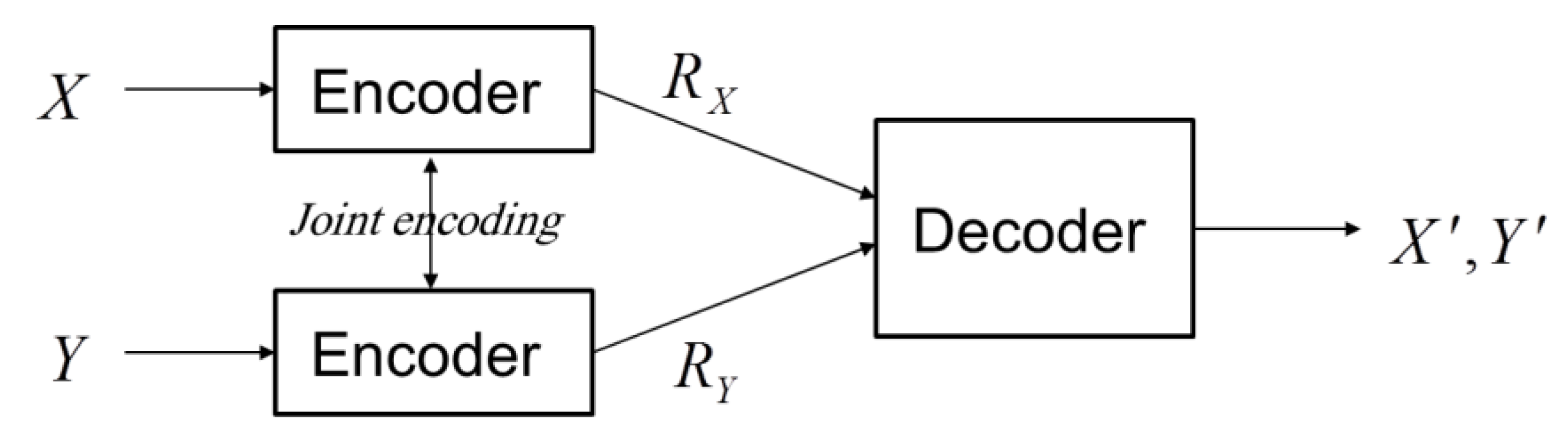
The Slepian–Wolf concept declares that the correlated sources, even if they do not directly communicate, may be encoded at a rate equal to their joint encoding rate without any loss in performance when decoded together. Figure 6 and Figure 7 provide visual representations of the difference between distributed encoding and joint encoding.

If the correlated sources are encoded individually and decoded together, the lowest data rate at which each data source is bound is as expressed below [37]:

$$\begin{array}{l}{R}_X+R_Y\ge H(X,Y)\\ R_X\ge H(X|Y)\\ R_Y\ge H(Y|X)\end{array}$$

(2)

In the context where R_x represents the rate of source x, R_y denotes the rate of source y, H(x/y) signifies the conditional entropy of x given y, H(y/x) indicates the conditional entropy of y given x, and H(x,y) represents the joint entropy of x and y, the entire data rate ought to be ≥ H(X, Y). Furthermore, the individual data rates should each be ≥H(X/Y) and H(Y/X), respectively.

3.4. Multi-Path Routing

For transmitting data from CHs toward the BS, multiple paths are established [38]. The phases involved in multi-path planning are as follows:

• Initialization Phase

During this phase, CHs broadcast a HELLO message to neighboring clusters, updating the neighboring table. Information regarding neighbors with the highest-quality data is retained. The HELLO message includes a hop count, representing the distance in hops from its initiator.

2.

Primary Path Discovery Phase

During the initialization phase, information for computing the cost function for neighboring sensors of CHs becomes accessible. Afterward, when the BS calculates the desired next hop CH, it dispatches an RREQ message to the most desired following hop. Similarly, the selected following hop CH of the BS calculates its most desired following the hop in the direction of the source sensor. An RREQ message is subsequently transmitted to the following hop, and this sequence persists up to reaching the source sensor.

3.

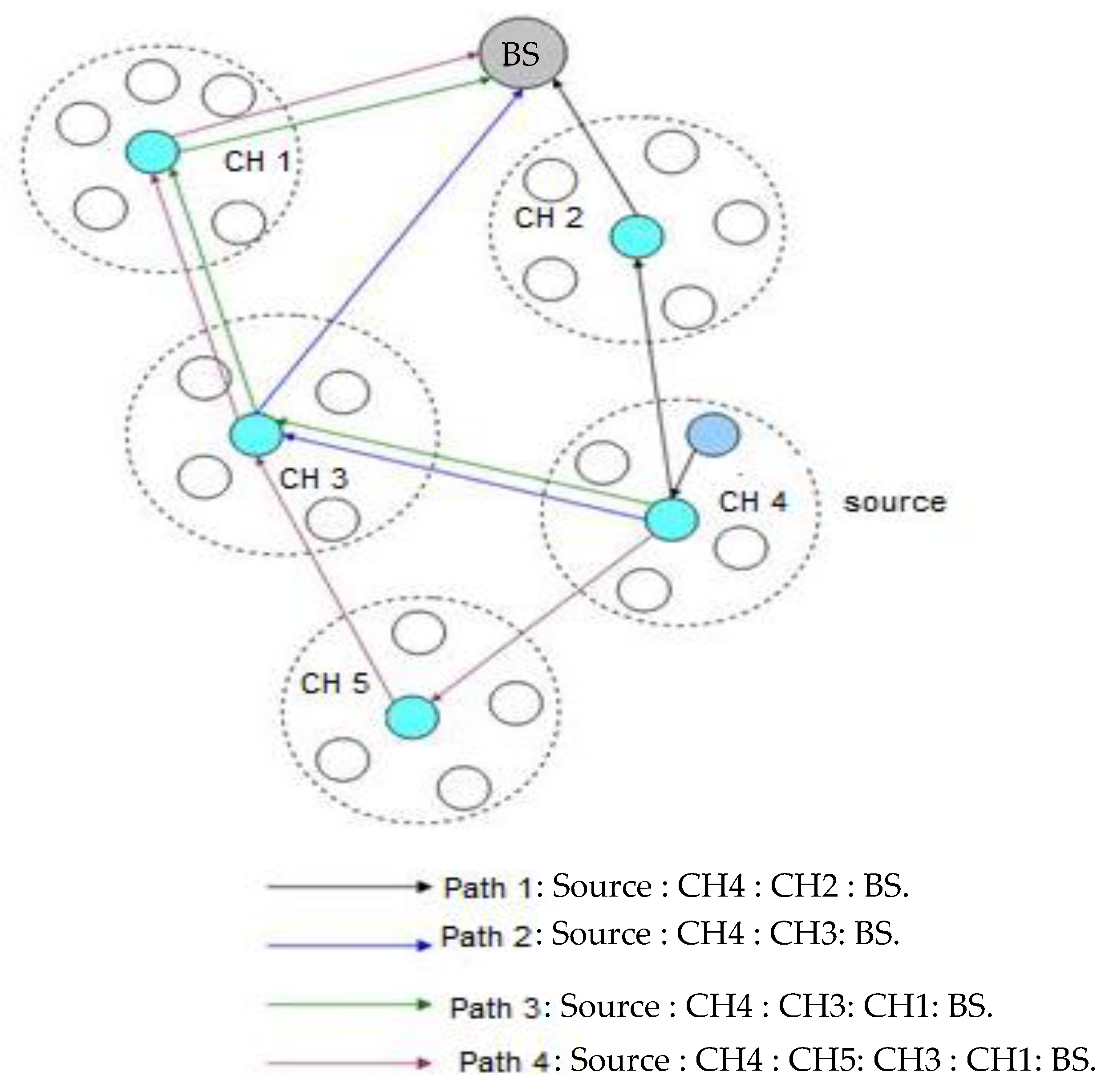
Alternative Paths Discovery Phase

The subsequent most favored neighbor is regarded as a substitute path, and the BS dispatches an alternative RREQ message to that neighbor. Each sensor exclusively approves one RREQ message to prevent paths with shared sensors. If multiple sensors receive one RREQ message, only the initial one is approved, disregarding the others. Multi-path routing from source at CH4 to BS is delineated in Figure 8.

The optimal path is determined by the minimum number of hops. Path 1 is selected for transmission between CH4 and BS, and the alternative path will be utilized in the event that the best path encounters a failure.

3.5. Mobility Models

Two mobility models are employed to assess the stability of the proposed algorithm and address the hot-spot issue.

3.5.1. Random Waypoint Mobility Algorithm

This algorithm simulates the movement patterns of mobile sensors on a freeway and is widely adopted by academic researchers. The application of this algorithm consists of the following steps:

• At each moment, a node selects a destination randomly and continues toward it with a velocity uniformly selected from the range [0, V_max], where V_max represents the maximum velocity allowed for each mobile sensor [39].
• Once the destination is reached, the sensor pauses for a period specified by the ‘pause time’ factor. Following this interval, it selects a new random endpoint and iterates the entire process up to the simulation terminates.

3.5.2. Reference Group Mobility Point

Sensor movement can be simulated using group mobility, described using the following equations [39]:

V_member(t) = V_leader(t) + SDR × max_speed

(3)

θ_member(t) = θ_leader(t) + ADR × max_angle

(4)

Here, 0 ≤ SDR, ADR ≤ 1. SDR denotes the Speed Deviation Ratio, and ADR signifies the Angle Deviation Ratio. These parameters are employed to regulate the deviation of the velocity (both magnitude and direction) of group members from that of the leader.

4. Simulation Results and Discussion

The MEDF algorithm underwent an evaluation using the NS2 simulator [40]. A random network installation within an area of 500 × 500 m² was taken into account, initially involving 250 nodes. The sink was installed 100 m away from the area considered. The variables used in the simulation are outlined in

Table 2. The variables used.

Variables	Magnitude
No. of nodes	10:250
Considered area size	500 × 500 m2
Mac	802.11
Routing protocol	MEDF
Run time	250 s
Source of traffic	Temperature application
Size of packet	500 bytes
Data rate	150 kbps
Communication range	100 m
Transmitting power	0.660 Watt
Receiving power	0.395 Watt
Optimal power	0.035 Watt
Start energy	10 J
Percentage of cluster heads	20%
No. of sources/cluster	4

.

The evaluation of the proposed MEDF algorithm is contrasted using EEMDF algorithm presented in [27]. Performance evaluation primarily focuses on the following metrics:

• PDR is calculated as the proportion of data packets received by the destinations to those generated by the sources.
• Network lifetime (NLT) is the count of nodes alive at the end of the simulation.
• Average energy consumed (AEC) is determined by dividing the total energy consumed across all nodes by the total number of nodes.
• Average delay (AD) is calculated as the ratio between the sum of all delays at each sensor and the total number of nodes.

During the initial simulation, we explored a range of sensors between 10 and 250, contrasting the Random Waypoint (RW) mobility algorithm with the Reference Point Group Mobility (RPGM) technique. We investigated the effects of increasing the nodes number on the mentioned metrics, beginning with the simulation outcomes for PDR.

4.1. Packet Delivery Ratio

Figure 9 and Figure 10 illustrate the outcomes of diverse simulation experiments assessing PDR across varying numbers of nodes for both the proposed MEDF and EEMDF [27] algorithms under RW and RPGM mobility scenarios, respectively. These figures demonstrate a decline in PDR as the number of nodes increases in both RW and RPGM mobility models. This decline is attributed to heightened traffic, leading to an increased likelihood of packet loss with larger node populations, specifically seen with the following:

• In the RW mobility model, the lowest PDR is observed at 250 sensors, with an increase of 2.39%, and the highest PDR occurs at 10 sensors, showcasing a MEDF enhancement of PDR by 6.39%, contrasted to EEMDF. Typically, MEDF boosts the PDR by 5.2%, contrasted to EEMDF.
• In the RPGM model, the lowest PDR is recorded at 250 sensors, with an increase of 6.1%, while the highest ratio is observed at 10 sensor nodes, demonstrating an MEDF improvement in PDR by 2% compared to EEMDF. On average, MEDF improves the PDR by 4%.

Table 3. PDR simulation results.

Number of Nodes	PDR Using RW (%)		Enhancement	PDR Using RPGM (%)		Enhancement
	EEMDF	MEDF	MEDF − EEMDF	EEMDF	MEDF	MEDF − EEMDF
10	84	90.4	6.4	96	98	2
25	83.6	88.9	5.3	94	97	3
50	82.8	87.2	4.4	93.5	95.4	1.9
75	82	87.1	5.1	93.2	96.7	3.5
100	81	86.2	5.2	92.2	96.2	4
150	79	86	7	90.6	96.1	5.5
200	80.1	85.8	5.7	89.8	96	6.2
250	78	80.4	2.4	89.7	95.8	6.1
Average			5.2%			4%

presents a summary of the simulation results for PDR.

4.2. Network Lifetime

Figure 11 displays the outcomes of diverse simulation tests assessing network lifetime across varying numbers of sensors for both MEDF and EEMDF algorithms. The figure demonstrates that as the number of network sensors increases, the network lifetime also increases for both MEDF and EEMDF.

In the RW mobility technique, the lowest lifetime of the network is observed at 10 sensors, where both MEDF and EEMDF exhibit identical lifetimes. Conversely, the highest lifetime of the network occurs at 250 sensors, with MEDF extending the lifetime of the network by 4.39%, contrasted to EEMDF. Thus, on average, MEDF extends the network lifetime by 4.3%, contrasted to EEMDF.

Figure 12 illustrates a similar trend, depicting an increase in network lifetime with a growing number of nodes for both MEDF and EEMDF. Under the RPGM mobility technique, the lowest lifetime of the network is observed at 10 sensors, with MEDF extending the network lifetime by 10%. Conversely, the highest lifetime occurs at 250 sensors, with MEDF extending the lifetime of the network by 6% contrasted to EEMDF. On average, MEDF extends the network lifetime by 13.9%.

Table 4. Network lifetime simulation results.

Number of Nodes	Number of Nodes Still Alive Using RW		Enhancement	Number of Nodes Still Alive Using RPGM		Enhancement
	EEMDF	MEDF	MEDF − EEMDF	EEMDF	MEDF	MEDF − EEMDF
10	9	9	90% − 90% = 0%	9	10	100% − 90% = 10%
25	13	14	56% − 52% = 4%	17	23	92% − 68% = 24%
50	35	36	72% − 70% = 2%	47	55	94% − 78% = 16%
75	54	55	73.3% − 72% = 1.3%	61	73	97% − 81% = 16%
100	68	75	75% − 68% = 7%	78	94	94% − 78% = 16%
150	97	111	74% − 64.6% = 9.4%	123	151	94% − 82% = 16%
200	120	132	66% − 60% = 6%	165	188	94% − 82.5% = 11.5%
250	198	209	83.6% − 79.2% = 4.4%	233	250	99% − 93% = 6%
Average			4.3%			13.9%

summarizes the simulation results presented in Figure 11 and Figure 12.

4.3. Average Energy Consumed

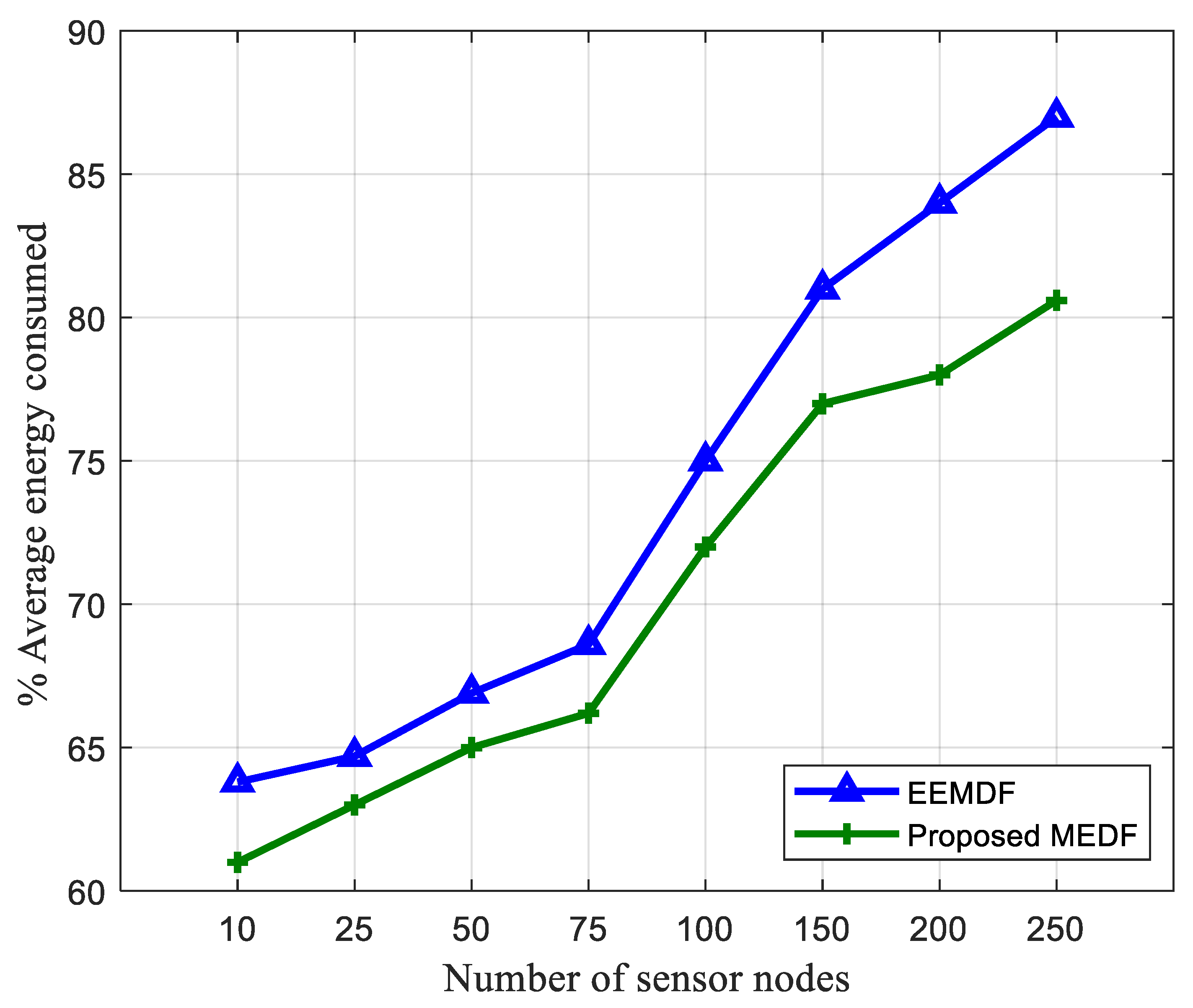
Figure 13 illustrates the findings of various simulation results measuring the average ratio of energy consumption at various numbers of sensors for MEDF and EEMDF, considering the RW mobility technique. As the number of sensors rises, the average energy consumed rises for both MEDF and EEMDF. The lowest ratio of average energy is observed at 10 sensors, with the ratio decreasing by 2.79%, and the largest average ratio occurs at 250 sensors, where MEDF reduces the ratio by 6.39%. Typically, MEDF achieves 3.52% more energy savings compared to EEMDF.

In Figure 14, the average ratio of energy consumption at various numbers of sensors is depicted for MEDF and EEMDF, considering the RPGM mobility technique. Similar to the RW mobility technique, the average energy consumed increases with the number of sensors in the network for both MEDF and EEMDF. The lowest ratio of average energy is observed at 10 sensors, with the ratio decreasing by 6%, and the largest average ratio occurs at 250 sensors, with MEDF reducing the ratio by 11%. Typically, MEDF achieves 7.70% more energy savings compared to EEMDF.

Table 5. Average energy consumed simulation results.

Number of Nodes	AEC Using RW (%)		Enhancement	AEC Using RPGM (%)		Enhancement
	EEMDF	MEDF	(EEMD − MEDF) %	EEMDF	MEDF	(EEMD − MEDF) %
10	63.8	61	2.8	61.8	55.8	6
25	64.7	63	1.7	62.7	55.7	7
50	66.9	65	1.9	64.9	58.6	6.3
75	68.6	66.2	2.4	66.6	60.3	6.3
100	75	72	3	73	67	6
150	81	77	4	79	69	10
200	84	78	6	82	73	9
250	87	80.6	6.4	86	75	11
Average			3.52%			7.70%

presents the summary of the obtained results from Figure 13 and Figure 14.

4.4. Average Delay

Figure 15 illustrates the findings of various experiments measuring the average delay versus the numbers of sensors for MEDF and EEMDF under the RW mobility technique. As the number of network sensors increases, the average delay also increases in both MEDF and EEMDF. The minimum average delay is observed at 10 sensors, with the ratio increasing by 0.0079%, while the largest average ratio occurs at 250 sensor nodes, where MEDF decreases the ratio by 0.07%. On average, MEDF incurs a delay increase of 0.05575% compared to EEMDF, which presents a disadvantage. However, considering the rise in PDR and network lifetime, a trade-off can be contemplated.

In Figure 16, the average delay versus numbers of sensors is depicted for MEDF and EEMDF, considering the RPGM mobility technique. Similar to the RW mobility model, the average delay increases as the number of sensors in the network increases for both MEDF and EEMDF. The lowest delay is observed at 10 sensor nodes, with the ratio increasing by 0.0039%, while the maximum delay occurs at 250 sensor nodes, with MEDF reducing the ratio by 0.02%. Typically, MEDF incurs a delay increase of 0.00975% compared to EEMDF, as indicated by

Table 6. Average delay simulation results.

Number of Nodes	Average Delay Using RW (Sec)		Enhancement	Average Delay Using RPGM (Sec)		Enhancement
	EEMDF	MEDF	MEMF − EEMDF	EEMDF	MEDF	MEMF − EEMDF
10	0.06	0.068	0.008	0.02	0.024	0.004
25	0.08	0.088	0.008	0.03	0.028	−0.002
50	0.1	0.17	0.07	0.04	0.048	0.008
75	0.3	0.38	0.08	0.05	0.056	0.006
100	0.5	0.59	0.09	0.06	0.069	0.009
150	0.7	0.76	0.06	0.07	0.073	0.003
200	0.9	0.96	0.06	0.11	0.14	0.03
250	1.1	1.17	0.07	0.13	0.15	0.02
Average			0.05575%			0.00975%

.

4.5. Performance Comparison

The experimental results presented above are used to validate the performance of the proposed MEDF algorithm against the EEMDF algorithm. In this subsection, we compare the performance of the proposed algorithm against other algorithms, such as the tracking-anchor-based clustering method (TACM) [41] and Energy-Efficient Dynamic Clustering (EEDC) Protocol [42]. We consider several metrics, such as average residual energy and network lifetime.

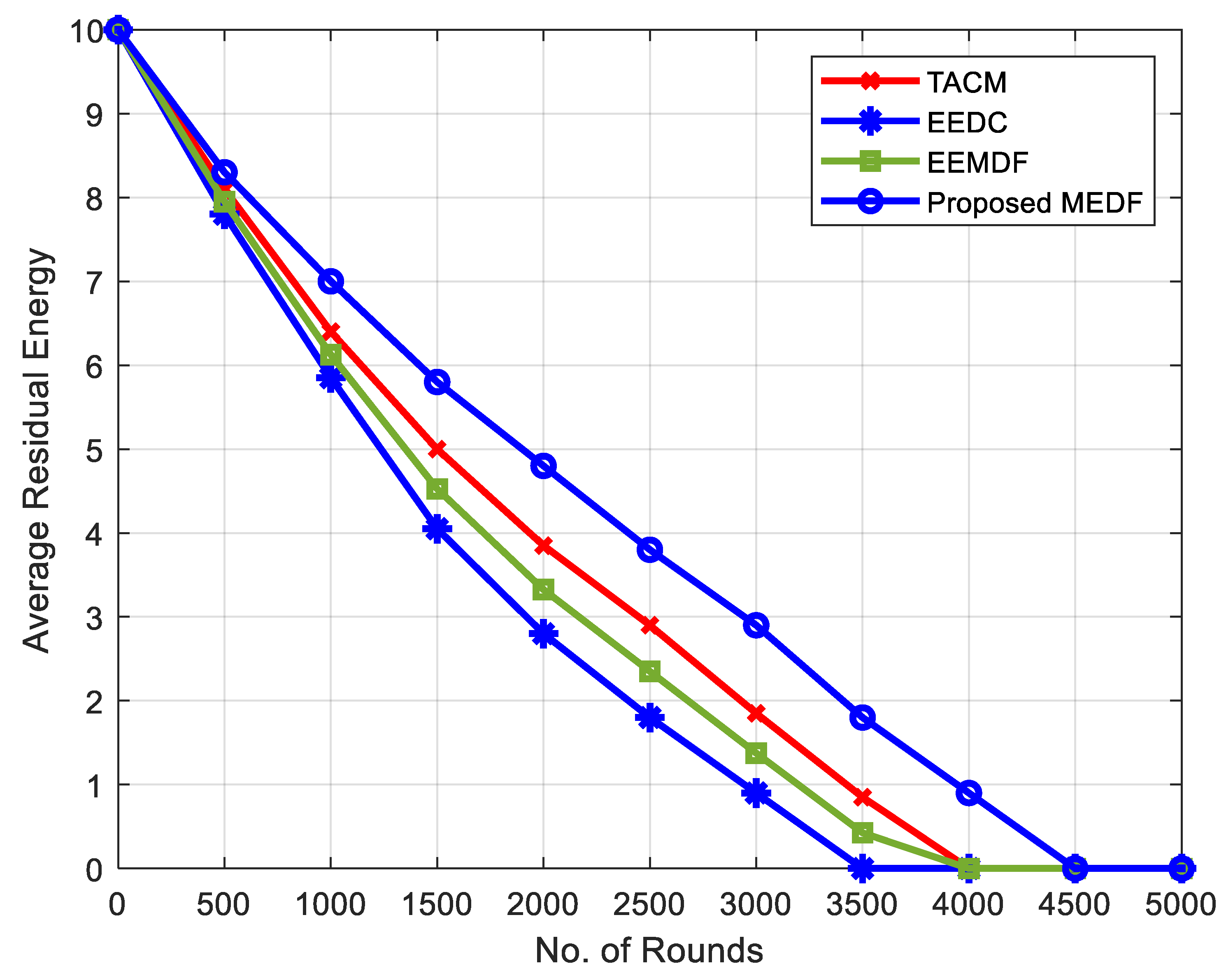
Figure 17 compares the average residual energy of the proposed MEDF, the EEMDF [27], the TACM [41], and the EEDC [42] algorithms. It is clear from this figure that the proposed algorithm achieves the best results when compared to the other algorithms. For example, at 1500 rounds, the average residual energy is 5.8 joules for the proposed MEDF, 5 joules for TACM, 4.525 joules for EEMDF, and 4.05 joules for EEDC.

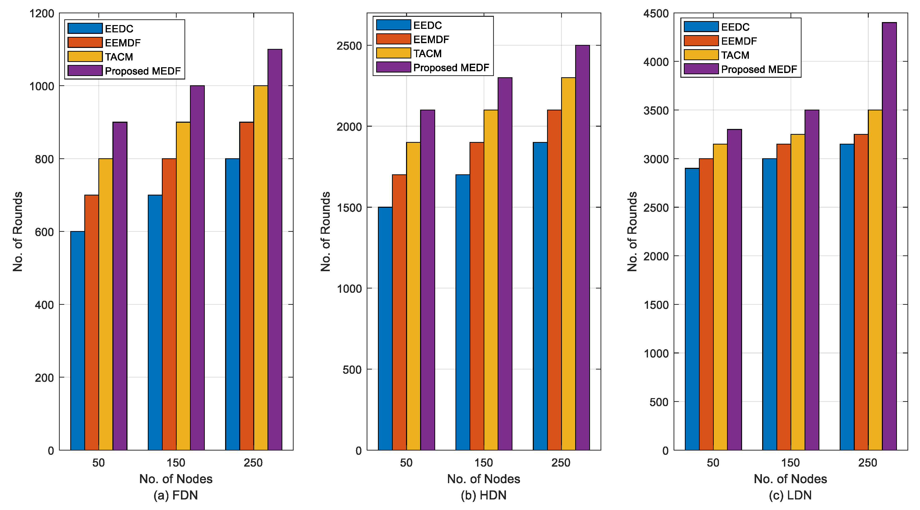
Figure 18 illustrates the network lifetime as a function of the number of nodes across three distinct scenarios: (a) First Dead Node (FDN), (b) Half Dead Node (HDN), and (c) Last Dead Node (LDN) [41]. As evident from the results, the proposed algorithm consistently outperforms the other algorithms in all scenarios.

4.6. Remarks on Experimental Results

The experimental results presented in the preceding sections demonstrate the effectiveness of the proposed MEDF algorithm in improving key performance metrics for WSNs. Here, we summarize and interpret the key observations:

• PDR: The MEDF algorithm achieves consistent improvements in PDR compared to the EEMDF algorithm across varying network sizes and mobility scenarios. This enhancement, averaging 5.2% under RW mobility and 4% under RPGM, highlights the robustness of the MEDF algorithm in ensuring reliable data delivery even in dense and dynamic network conditions.
• Network lifetime: The proposed algorithm significantly extends network lifetime, with average improvements of 4.3% under RW mobility and 13.9% under RPGM. This demonstrates the effectiveness of adaptive clustering and load balancing in mitigating energy depletion, particularly in hot spot-prone areas near the base station.
• Energy efficiency: MEDF consistently reduces average energy consumption compared to EEMDF, with savings of 3.52% under RW mobility and 7.7% under RPGM. These results confirm the efficiency of the data-compression and -clustering techniques in optimizing resource utilization.
• Average delay: While MEDF achieves notable improvements in other metrics, it incurs a slight increase in average delay compared to EEMDF (0.05575% under RW mobility and 0.00975% under RPGM). This trade-off is considered acceptable given the substantial gains in PDR, energy efficiency, and network longevity.
• Average residual energy: The comparison of the average residual energy for the proposed MEDF algorithm against EEMDF [27], TACM [41], and EEDC [42] highlights its superior performance. For instance, after 1500 rounds, the average residual energy is 5.8 joules for MEDF, compared to 5 joules for TACM, 4.525 joules for EEMDF, and 4.05 joules for EEDC. These results emphasize the MEDF algorithm’s ability to conserve energy more effectively.

5. Conclusions

The introduction of the MEDF algorithm within the presented WSN topology marks a significant advancement toward energy-efficient information dissemination. Through the integration of data-compression protocols and adaptive-clustering mechanisms, the presented topology aims to address key challenges, such as network longevity, PDR, and the mitigation of hot-spot issues. Cluster head selection is based on residual energy, ensuring that nodes join cluster heads to minimize communication overhead. Additionally, we enhanced our topology with an RPGM technique to mitigate the hot-spot problem. The simulation results have demonstrated the effectiveness of the MEDF algorithm, showcasing improvements in PDR and energy efficiency compared to the EEMDF algorithm. Specifically, the proposed MEDF algorithm achieves gains of 5.2% and 7.7% in PDR and energy efficiency, respectively, while extending network lifetime by 13.9%. However, it is noted that a slight increase in delay, by 0.01% compared to EEMDF, is observed. Finally, the proposed algorithm was compared to other algorithms, such as TACM and EEDC, and the obtained results emphasize the MEDF algorithm’s ability to conserve energy more effectively, contributing to its extended network lifetime.

As such, future research efforts may focus on further refining the algorithm and exploring its applicability in diverse WSN environments. Additionally, investigations into optimizing delay performance while maintaining energy efficiency would be beneficial for advancing the practical implementation of the MEDF algorithm in real-world scenarios.

References

- Hassan, E.S. Energy-Efficient Resource Allocation Algorithm for CR-WSN-Based Smart Irrigation System under Realistic Scenarios. Agriculture 2023, 13, 1149. [Google Scholar] [CrossRef]
- Alharbi, F.; Zakariah, M.; Alshahrani, R.; Albakri, A.; Viriyasitavat, W.; Alghamdi, A.A. Intelligent Intelligent Transportation Using Wireless Sensor Networks Blockchain and License Plate Recognition. Sensors 2023, 23, 2670. [Google Scholar] [CrossRef] [PubMed]
- Khan, A.U.; Khan, M.E.; Hasan, M.; Zakri, W.; Alhazmi, W.; Islam, T. An Efficient Wireless Sensor Network Based on the ESP-MESH Protocol for Indoor and Outdoor Air Quality Monitoring. Sustainability 2022, 14, 16630. [Google Scholar] [CrossRef]
- Prashar, D.; Rashid, M.; Siddiqui, S.T.; Kumar, D.; Nagpal, A.; AlGhamdi, A.S.; Alshamrani, S.S. SDSWSN—A Secure Approach for a Hop-Based Localization Algorithm Using a Digital Signature in the Wireless Sensor Network. Electronics 2021, 10, 3074. [Google Scholar] [CrossRef]
- Hassan, E.S.; Oshaba, A.S.; Elemary, A.; Elsafrawey, A. Enhancing the Lifetime and Performance of WSNs in Smart Irrigation Systems using Cluster-Based Selection Protocols. Irrig. Drain. 2023, 72, 1109–1123. [Google Scholar] [CrossRef]
- Shuaib, M.; Bhatia, S.; Alam, S.; Masih, R.K.; Alqahtani, N.; Basheer, S.; Alam, M.S. An Optimized, Dynamic, and Efficient Load-Balancing Framework for Resource Management in the Internet of Things (IoT) Environment. Electronics 2023, 12, 1104. [Google Scholar] [CrossRef]
- Alam, S.; Bhatia, S.; Shuaib, M.; Khubrani, M.M.; Alfayez, F.; Malibari, A.A.; Ahmad, S. An Overview of Blockchain and IoT Integration for Secure and Reliable Health Records Monitoring. Sustainability 2023, 15, 5660. [Google Scholar] [CrossRef]
- Barat, A.; Prabuchandran, K.J.; Bhatnagar, S. Energy Management in a Cooperative Energy Harvesting Wireless Sensor Network. IEEE Commun. Lett. 2024, 28, 243–247. [Google Scholar] [CrossRef]
- Yoon, I.; Noh, D.K. Adaptive Data Collection Using UAV With Wireless Power Transfer for Wireless Rechargeable Sensor Networks. IEEE Access 2022, 10, 9729–9743. [Google Scholar] [CrossRef]
- Naghibzadeh, M.; Taheri, H.; Neamatollahi, P. Fuzzy-based clustering solution for hot spot problem in wireless sensor networks. In Proceedings of the 7’th International Symposium on Telecommunications (IST’2014), Tehran, Iran, 9–11 September 2014; pp. 729–734. [Google Scholar] [CrossRef]
- Jing, D. Harris Harks Optimization Based Clustering With Fuzzy Routing for Lifetime Enhancing in Wireless Sensor Networks. IEEE Access 2024, 12, 12149–12163. [Google Scholar] [CrossRef]
- Wang, J.; Wang, N.; Sun, B.; Cao, K.; Jung, K.; El-Meligy, M.A. An Improved Data Fusion Algorithm Based on Cluster Head Election and Grey Prediction. IEEE Access 2024, 12, 22746–22758. [Google Scholar] [CrossRef]
- Ahmed, A.; Parveen, I.; Abdullah, S.; Ahmad, I.; Alturki, N.; Jamel, L. Optimized Data Fusion With Scheduled Rest Periods for Enhanced Smart Agriculture via Blockchain Integration. IEEE Access 2024, 12, 15171–15193. [Google Scholar] [CrossRef]
- Qaffas, A.A. Optimized Back Propagation Neural Network Using Quasi-Oppositional Learning-Based African Vulture Optimization Algorithm for Data Fusion in Wireless Sensor Networks. Sensors 2023, 23, 6261. [Google Scholar] [CrossRef] [PubMed]
- Anees, J.; Zhang, H.-C.; Baig, S.; Guene Lougou, B.; Robert Bona, T.G. Hesitant Fuzzy Entropy-Based Opportunistic Clustering and Data Fusion Algorithm for Heterogeneous Wireless Sensor Networks. Sensors 2020, 20, 913. [Google Scholar] [CrossRef]
- Irfan, S.; Ramesh, K.S.; Kumar, N.S.; Maheswary, A. Battery Lifetime Enhancement in Wireless Sensor Networks using Artificial Intelligence Techniques. In Proceedings of the 2021 3rd International Conference on Advances in Computing, Communication Control and Networking (ICAC3N), Greater Noida, India, 17–18 December 2021; pp. 1283–1288. [Google Scholar] [CrossRef]
- Meng, J.-T.; Yuan, J.-R.; Feng, S.-Z.; Wei, Y.-J. An Energy Efficient Clustering Scheme for Data Aggregation in Wireless Sensor Networks. J. Comput. Sci. Technol. 2013, 28, 564–573. [Google Scholar] [CrossRef]
- Ghazy, A.S.; Kaddoum, G.; Singh, S. Low-Latency Low-Energy Adaptive Clustering Hierarchy Protocols for Underwater Acoustic Networks. IEEE Access 2023, 11, 50578–50594. [Google Scholar] [CrossRef]
- Priyadarshi, R.; Singh, L.; Randheer; Singh, A. A Novel HEED Protocol for Wireless Sensor Networks. In Proceedings of the 2018 5th International Conference on Signal Processing and Integrated Networks (SPIN), Noida, India, 22–23 February 2018; pp. 296–300. [Google Scholar] [CrossRef]
- Nedham, W.B.; Kadhum, A.; Al-Qurabat, M. An Improved Energy Efficient Clustering Protocol for Wireless Sensor Networks. In Proceedings of the 2022 International Conference for Natural and Applied Sciences (ICNAS), Baghdad, Iraq, 14–15 May 2022; pp. 23–28. [Google Scholar] [CrossRef]
- Sinha, A.; Lobiyal, D.K. A Dynamic Aggregation Protocol for Energy Efficient Data Fusion in Wireless Sensor Network. Int. J. Comput. Appl. 2011, 16, 32–38. [Google Scholar] [CrossRef]
- Xu, Y.; Sun, G.; Geng, T.; Li, Z. Compressive Multi-Timeslots Data Gathering With Total Variation Regularization for Wireless Sensor Networks. IEEE Commun. Lett. 2019, 23, 648–651. [Google Scholar] [CrossRef]
- Sudheer, B.N.; Sujatha, K. A Brief Survey on Data Aggregation and Data Compression Models using Blockchain Model in Wireless Sensor Network. In Proceedings of the 2023 International Conference on Innovative Data Communication Technologies and Application (ICIDCA), Uttarakhand, India, 14–16 March 2023; pp. 406–413. [Google Scholar] [CrossRef]
- Kirton, J.; Bradbury, M.; Jhumka, A. Source Location Privacy-Aware Data Aggregation Scheduling for Wireless Sensor Networks. In Proceedings of the 2017 IEEE 37th International Conference on Distributed Computing Systems (ICDCS), Atlanta, GA, USA, 5–8 June 2017; pp. 2200–2205. [Google Scholar] [CrossRef]
- Deepakraj, D.; Raja, K. Hybrid Data Aggregation Algorithm for Energy Efficient Wireless Sensor Networks. In Proceedings of the 2021 Third International Conference on Intelligent Communication Technologies and Virtual Mobile Networks (ICICV), Tirunelveli, India, 4–6 February 2021; pp. 7–12. [Google Scholar] [CrossRef]
- Sethi, H.; Prasad, D.; Patel, R.B. EIRDA: An Energy Efficient Interest based Reliable Data Aggregation Protocol for Wireless Sensor Networks. Int. J. Comput. Appl. 2011, 22, 20–25. [Google Scholar] [CrossRef]
- Sasikala, G.; Chandraseka, C. Energy Efficient Multipath Data Fusion Technique for Wireless Sensor Networks. ACEEE Int. J. Netw. Secur. 2012, 3, 34–41. [Google Scholar]
- Tabella, G.; Ciuonzo, D.; Yilmaz, Y.; Wang, X.; Rossi, P.S. Time-aware distributed sequential detection of gas dispersion via wireless sensor networks. IEEE Trans. Signal Inf. Process. Over Netw. 2023, 9, 721–735. [Google Scholar] [CrossRef]
- Hua, Y.; Gan, H.; Wan, F.; Qin, X.; Liu, F. Distributed estimation with adaptive cluster learning over asynchronous data fusion. IEEE Trans. Aerosp. Electron. Syst. 2023, 59, 5262–5274. [Google Scholar] [CrossRef]
- Wu, L.; Sahu, N.; Xu, S.; Babu, P.; Ciuonzo, D. Optimization based sensor placement for multi-target localization with coupling sensor clusters. IEEE Trans. Signal Inf. Process. Over Netw. 2023, 9, 596–611. [Google Scholar] [CrossRef]
- Zhang, J.; Yan, R. Multi-objective Distributed Clustering Algorithm in Wireless Sensor Networks Using the Analytic Hierarchy Process. In Proceedings of the 2019 20th IEEE/ACIS International Conference on Software Engineering, Artificial Intelligence, Network-ing and Parallel/Distributed Computing (SNPD), Toyama, Japan, 8–11 July 2019; pp. 88–93. [Google Scholar] [CrossRef]
- Chinh, D.C.; Kumar, R.; Panda, S.K. Optimal Data Aggregation Tree in Wireless Sensor Networks Based on Intelligent Water Drops Algorithm. IET Wirel. Sens. Syst. 2011, 2, 282–292. [Google Scholar] [CrossRef]
- Pal, V.; Singh, G.; Yadav, R.P.; Pal, P. Energy Efficient Clustering Scheme for Wireless Sensor Networks: A Survey. J. Wirel. Netw. Commun. 2012, 2, 168–174. [Google Scholar] [CrossRef]
- Hassan, E.S. Three layer hybrid PAPR reduction method for NOMA-based FBMC-VLC networks. Opt. Quant. Electron. 2024, 56, 890. [Google Scholar] [CrossRef]
- Xiao, D.; Tang, Q.; Zhao, A.; Li, M. Robust Watermarking Scheme in Encrypted Domain Based on Integer Lifting Wavelet Transform and Compressed Sensing. In Proceedings of the ICASSP 2023-2023 IEEE International Conference on Acoustics, Speech and Signal Processing (ICASSP), Rhodes Island, Greece, 4–10 June 2023; pp. 1–5. [Google Scholar] [CrossRef]
- Mbewe, P.; Asare, S.D. Analysis and comparison of adaptive huffman coding and arithmetic coding algorithms. In Proceedings of the 2017 13th International Conference on Natural Computation, Fuzzy Systems and Knowledge Discovery (ICNC-FSKD), Guilin, China, 29–31 July 2017; pp. 178–185. [Google Scholar] [CrossRef]
- Wang, W.; Shin, S. A distributed source rate control optimization approach in energy harvesting wireless sensor networks. In Proceedings of the 2013 22nd Wireless and Optical Communication Conference, Chongqing, China, 16–18 May 2013; pp. 410–414. [Google Scholar] [CrossRef]
- Roopa, D.; Chaudhari, S. A survey on Geographic Multipath Routing Techniques in Wireless Sensor Networks. In Proceedings of the 2019 5th International Conference on Advanced Computing & Communication Systems (ICACCS), Coimbatore, India, 15–16 March 2019; pp. 257–262. [Google Scholar] [CrossRef]
- Sakaguchi, R.; Matsui, D.; Nakamura, R.; Ohsaki, H. Analysis of Constrained Random WayPoint Mobility Model on Graph. In Proceedings of the 2020 International Conference on Information Networking (ICOIN), Barcelona, Spain, 7–10 January 2020; pp. 312–317. [Google Scholar] [CrossRef]
- Krishna, K.H.; Kumar, T.; Babu, Y.S. Energy effectiveness practices in WSN over simulation and analysis of S-MAC and leach using the network simulator NS2. In Proceedings of the 2017 International Conference on I-SMAC (IoT in Social, Mobile, Analytics and Cloud) (I-SMAC), Palladam, India, 10–11 February 2017; pp. 914–920. [Google Scholar] [CrossRef]
- Qu, Z.; Li, B. An Energy-Efficient Clustering Method for Target Tracking Based on Tracking Anchors in Wireless Sensor Networks. Sensors 2022, 22, 5675. [Google Scholar] [CrossRef] [PubMed]
- Qu, Z.; Xu, H.; Zhao, X.; Tang, H.; Wang, J.; Li, B. An Energy-Efficient Dynamic Clustering Protocol for Event Monitoring in Large-Scale WSN. IEEE Sens. J. 2021, 21, 23625. [Google Scholar] [CrossRef]
Figure 1.
The main steps of MEDF algorithm.
Figure 2.
Proposed cluster-formation algorithm.
Figure 3.
Data fusion steps.
Figure 4.
LWT procedures.
Figure 5.
Multi-level LWT procedures.
Figure 6.
Visual representation of distributed encoding.
Figure 7.
Visual representation of joint encoding.
Figure 8.
Multi-path routing from source at CH4 to BS.
Figure 9.
PDR of MEDF and EEMDF [
27] algorithms using RW mobility technique.
Figure 10.
27] algorithms using RPGM mobility technique.
Figure 11.
Network lifetime using RW mobility technique.
Figure 12.
Network lifetime using RPGM mobility technique.
Figure 13.
AEC using RW mobility technique.
Figure 14.
AEC using the RPGM mobility technique.
Figure 15.
Average delay using RW mobility technique.
Figure 16.
Average delay using RPGM mobility technique.
Figure 17.
Average residual energy versus number of rounds for the considered algorithms.
Figure 18.
Network lifetime versus number of nodes: (a) First Dead Node, (b) Half Dead Node, and (c) Last Dead Node.