Article

Deterministic and Stochastic Modeling of Deposit–Loan Dynamics with Optimal Regulatory Control

by
Moch. Fandi Ansori
1,*,
F. Hilal Gümüş
2,
Ratna Herdiana
1,
Hafidh Khoerul Fata
1,
Nurcahya Yulian Ashar
1 and
Handika Lintang Saputra
1
1
Department of Mathematics, Faculty of Science and Mathematics, Universitas Diponegoro, Semarang 50275, Indonesia
2
Department of Business Administration, Faculty of Economics and Administrative Science, Zonguldak Bülent Ecevit University, Zonguldak 67100, Türkiye
*
Author to whom correspondence should be addressed.
Int. J. Financial Stud. 2026, 14(7), 174; https://doi.org/10.3390/ijfs14070174
Submission received: 15 May 2026 / Revised: 1 July 2026 / Accepted: 3 July 2026 / Published: 6 July 2026
(This article belongs to the Special Issue Mathematical Finance: Theory, Methods, and Applications)

Abstract

Banks must balance deposit stability, loan expansion, and regulatory compliance while operating under liquidity constraints and financial risks. This study presents a mathematical model to examine the dynamics of bank deposits and loans under the influence of liquidity mechanisms and regulatory policies. The model proceeds in three stages: a deterministic nonlinear model, a dynamic optimal control model, and a stochastic model. Under the deterministic model, deposit withdrawals are liquidity-dependent, leading to a feedback mechanism in which liquidity improves deposit stability while financing loan growth. The theoretical results demonstrate the model’s positive and bounded solutions and show the existence and local stability of equilibria. Several parameters are based on regulatory policies or calibrated from Indonesian banking data, while the unknown parameters are estimated using the particle swarm optimization (PSO) algorithm. The results show that the proposed model is capable of fitting and predicting the data and has slightly lower mean absolute percentage errors for in-sample and out-of-sample compared with the benchmark model, and achieves comparable directional forecasting performance based on the index of directionality. Sensitivity analysis shows that the capital adequacy ratio supports lending, whereas an increased reserve requirement limits lending. An optimal control approach is developed by considering the reserve and capital requirements as time-varying policy variables. By applying Pontryagin’s maximum principle, we establish the necessary conditions for optimality. Numerical experiments demonstrate that the optimal control regulation enhances financial ratios, particularly the loan-to-deposit and liquidity ratios, at a reasonable cost. Finally, the stochastic model accounts for random variations in withdrawals and credit risks. Simulation-based observations reveal that although the system becomes more volatile, the mean dynamics are close to the deterministic case. Our framework offers a data-based and analytically tractable approach for studying the dynamics of banking variables and the effects of regulatory policies. The proposed model provides a mathematical tool for assessing the long-term effects of regulatory policies on banking performance and can assist bank managers and regulators in designing strategies that balance lending activity and liquidity resilience.

1. Introduction

The stability of the banking sector is fundamental to modern financial systems for promoting economic activity, investment, and shock absorption. At the heart of stability lies the interaction between deposit funding and lending, which affects liquidity, credit provision, and banks’ resilience to shocks (Al-Shimmery, 2019; Kashyap et al., 2002). Liquidity management involves balancing deposit withdrawals and loan disbursements while maintaining sufficient liquid assets to manage withdrawal risk and fund credit operations. Deposits provide the funding that is essential for maintaining loan supply in response to liquidity shocks, and core deposits are particularly vital in this regard, while deposit composition and contractual terms affect risk management and lending practices (Dutto Giolongo & Carlevaro, 2019; Jung & Kim, 2015; Qiu, 2011; D. V. Tran, 2020). However, deposit funding may also constrain credit growth, particularly in situations of funding uncertainty and regulatory pressure, suggesting that deposit funding is both a stabilizing and constraining element in banking (Ábel & Mérő, 2023; Carletti et al., 2021; Mallett, 2012; Ritz & Walther, 2015; D. V. Tran, 2020). Additionally, credit lines, relationship lending, and interbank connections play a role in liquidity management, offering protection against funding constraints but also serving as vehicles for risk contagion in the banking system (Acharya et al., 2020; Bräuning & Fecht, 2017; Cappelletti & Mistrulli, 2023; Cocco et al., 2009; Temizsoy et al., 2015).
These funding–lending dynamics are important for financial stability because funding–lending mismatches can amplify systemic risk. Theoretical and empirical evidence shows a strong two-way link, with shocks to deposits impacting credit and shocks to lending affecting deposits (Al-Shimmery, 2019; De Moraes et al., 2015; Hossain et al., 2013; Song & Thakor, 2007). The impacts of non-performing loans, market liquidity, and bank market power further complicate this dynamic, influencing both credit supply and financial stability (Adebisi et al., 2018; Ally et al., 2025; Dombret et al., 2019; Gunay, 2020; Mohammed, 2025; Neziraj Elshani, 2025). While stable deposit-based funding improves crisis resilience relative to wholesale funding, the impact of this mechanism is contingent on macroeconomic, institutional, and regulatory factors (Boamah et al., 2023; De Haas & Van Lelyveld, 2014; Košak et al., 2015; Liu et al., 2025; H. S. Tran et al., 2023). While there is a wealth of empirical evidence, there is a need to further understand the dynamic and nonlinear relationship between deposits and loans, especially under uncertainty and structural shifts (Chand et al., 2024; Neziraj Elshani, 2025; Talavera et al., 2012). Recognizing these limitations, the need for integrated data-driven mathematical models capable of capturing complex banking dynamics and providing insights into regulatory policies has emerged.
Mathematical models are increasingly used to study financial systems. Dynamical system models can capture nonlinear interactions and feedback dynamics in financial and banking systems. These models have been used to examine banking activities, including risk, loan default, and profitability under different economic scenarios (Abdukadyrova et al., 2024; Gümüş & Ansori, 2026; Rumiantsev, 2008), and interbank interactions and systemic risks using network models (Ansori et al., 2021; Antonio et al., 2025; Cappelletti & Mistrulli, 2023). Models that use stochastic differential equations, optimal control, and nonlinear dynamics have been applied to explore systemic risk, contagion, and policymaking in financial networks (Ansori, 2026; Bauso et al., 2026; Fatone & Mariani, 2020; Neamah et al., 2025; Zhang et al., 2026). Moreover, models that consider economic and behavioral aspects allow for greater realism (Zakharov et al., 2025). The policy implications of dynamic models include the impact of monetary policies, such as interest rates and reserve requirements, on bank stability and credit dynamics (Gao et al., 2025).
Previous studies have used continuous and discrete-time models to study banking dynamics with respect to loan dynamics, interest rate policies, and banking competition. Analytical models employing gradient adjustment and bifurcation theory indicate that banking regulations and factors can destabilize loan equilibria and even lead to chaotic dynamics (Ansori et al., 2025, 2024; Ansori & Hariyanto, 2022; Ansori & Khabibah, 2022). However, Markov models that incorporate customer behavior and credit risk offer more realistic forecasts of loan portfolio dynamics (Bozhalkina, 2017; Timofeeva et al., 2018). Studies on interest rate policies show that competition increases the transmission of monetary policy through lower loan rates, while unconventional policies (such as negative interest rates) can increase lending while destabilizing the banking system (Leroy & Lucotte, 2015; Pedrosa & Mansilla Fernández, 2020; van Leuvensteijn et al., 2013). Additionally, banking competition plays a key role in risk-taking, with reduced market power increasing loan risk in a low-interest-rate environment and deregulation exacerbating regional monetary policy effects (Huynh, 2025; Segev & Schaffer, 2020; Shikimi, 2023). However, many models are based on assumptions such as fixed withdrawal rates and exogenous liquidity, which may not reflect actual banking operations.
Liquidity in banking systems serves a dual purpose by facilitating credit creation and increasing depositor trust, thus establishing a link between deposits and lending. Liquidity supports lending, but it can also lead to risk (Bleck & Liu, 2018; Chauhan & Sharma, 2025). These interactions can be represented by a stress-test model (Costa et al., 2021). Regulatory measures, such as reserve requirements and banking regulations, also affect these dynamics through their impact on liquidity allocation and lending (Chawwa, 2021; Ling et al., 2022; M’bakob & Tchounga, 2024; Sharma, 2026). As such, holistic models are required to describe the interactions among liquidity, regulation, and banking activity (Hodula et al., 2021).
Considering these factors, this study proposes a data-driven nonlinear dynamical model for banking deposits and loans. The model captures liquidity-sensitive withdrawal dynamics and regulatory rules, enabling liquid assets to affect deposit stability and bank lending. The model parameters were calibrated using data from Indonesian commercial banks, employing a particle swarm optimization (PSO) algorithm to accurately reflect real-world banking dynamics. This approach broadly aligns with (Lampart et al., 2023), who developed a deterministic nonlinear model of bank share price dynamics influenced by risk and market sentiment and validated it using empirical financial time-series data.
This study was conducted in three complementary stages. First, we developed a deterministic model and examined its properties, including positivity, boundedness, equilibrium points, and local stability. Second, the model is expanded into an optimal control model in which reserve requirements and capital adequacy ratios are time-varying policy variables. Using Pontryagin’s maximum principle, we find the necessary conditions for an optimal regulatory policy. Third, we extend the model to a stochastic setting by introducing random shocks to withdrawals and credit risk.
This study makes three contributions. First, from a theoretical perspective, we develop a novel deterministic mathematical model of liquidity-based banking dynamics that explicitly captures the interactions among deposits, loans and available liquidity. Second, we incorporate reserve requirements and capital adequacy ratio policies into an optimal control model, providing a mathematical basis for determining dynamic regulatory policies and assessing their effects on key financial indicators, such as loan-to-deposit and liquidity ratios. Third, we extend the deterministic model to a stochastic model by incorporating random fluctuations in withdrawals and credit risk, thereby enabling an analysis of the uncertainty in banking operations. From a practical standpoint, the proposed model is calibrated using Indonesian banking data and can be used by regulators and bank managers to evaluate the consequences of changes in regulatory policies, design strategies that balance lending activity and liquidity resilience, and assess banking performance under uncertain economic conditions.
The remainder of this paper is structured as follows. Specifically, Section 2 details the deterministic model and dynamics, as well as parameter estimation and sensitivity analysis. Section 3 presents the optimal control problem and the numerical results. Section 4 presents the stochastic model and its dynamics. Finally, Section 5 concludes the paper and provides suggestions for future work.

2. Deterministic Model

2.1. Model Formulation

We consider a balance sheet structure with deposits and equity on the liability side and loans, central bank reserves, and liquid assets on the asset side. Let D be the deposits, E the bank’s equity, L the loans, R the reserves, and A the bank’s liquid assets that can be used to lend money.
Under this balance-sheet structure, total assets must equal total liabilities, which implies
L + R + A = D + E .
Rearranging this identity yields
A = D + E L R .
Following regulatory conventions, equity is assumed to be proportional to the loan portfolio,
E = ( c + b ) L ,
where c denotes the regulatory minimum capital adequacy ratio, and b is the bank-specific capital buffer above the minimum, held by the bank. Furthermore, reserves are assumed to be proportional to deposits,
R = r D ,
where r ( 0 , 1 ) represents the reserve–requirement ratio.
Substituting these expressions into the definition of liquid assets gives
A = D + ( c + b ) L L r D = ( 1 r ) D + ( c + b 1 ) L .
Following the recent study by Ansori et al. (2025), the time dynamics of the deposits D ( t ) and loans L ( t ) are considered in a banking system, as described by the following system of differential equations:
d D d t = a D D 1 D K D w D ,
d L d t = a L A L 1 L K L η L δ ( 1 η ) L ,
where a D and a L represent the intrinsic growth rates of deposits and loans, respectively, and K D and K L are the respective carrying capacities. The parameters w, η , and δ denote the withdrawal, non-performing loan, and loan repayment rates, respectively.
Although the withdrawal rate is normally assumed to be constant (Ansori, 2026; Ansori et al., 2025), we assume that deposit withdrawals are correlated with bank liquidity. Specifically, liquidity is expected to enhance depositor trust and reduce withdrawals. This assumption is motivated by the bank-run framework of Diamond and Dybvig (1983). For this purpose, we assume that the withdrawal rate is a linear function of liquid assets:
w = w 0 ϕ A ,
where w 0 > 0 is the baseline withdrawal rate, and ϕ > 0 measures the sensitivity of withdrawals to liquidity conditions. A higher level of liquid assets reduces the effective withdrawal rate, thereby reflecting improved funding stability.
Substituting this expression into the deposit equation yields
d D d t = a D D 1 D K D ( w 0 ϕ A ) D .
Accordingly, the final model can be written as
d D d t = a D D 1 D K D w 0 D + ϕ A D ,
d L d t = a L A L 1 L K L η L δ ( 1 η ) L ,
where A is given by (1).
In (5), A is interpreted as liquid assets available for lending. Under the condition c + b < 1 , the expression for A in (1) may become negative for sufficiently high loans relative to deposits. Thus, the feasible region for A 0 is required to be determined. This condition is equivalent to the total deposit and equity after paying the reserve requirement being greater than the loan volume, that is,
D R + E = ( 1 r ) D + ( c + b ) L L .
Similarly, the withdrawal rate w = w 0 ϕ A may become negative when liquidity is high. Therefore, we need to constrain w 0 . This is equivalent to
A w 0 ϕ .
The proposed model reflects the relationship between bank funding stability and loan growth. Loan expansion is based on liquid assets from deposits and bank capital. In contrast, deposit stability is enhanced by greater liquidity, as reflected by the reduction in withdrawal pressure in response to increased liquid assets. Thus, the framework represents a duality between liquidity supporting loan growth and improving deposit stability.

2.2. Positivity and Boundedness of Solutions

In this subsection, the positivity and boundedness of the system solutions (4) and (5) are analyzed. The model can be written in the form
d D d t = D F ( D , L ) , d L d t = L G ( D , L ) ,
where
F ( D , L ) = a D 1 D K D w 0 + ϕ ( 1 r ) D + ( c + b 1 ) L , G ( D , L ) = a L ( 1 r ) D + ( c + b 1 ) L 1 L K L η δ ( 1 η ) .
This multiplicative structure is essential for establishing the positivity of the solutions.
Theorem 1.
Assume that the initial conditions satisfy
D ( 0 ) = D 0 > 0 , L ( 0 ) = L 0 > 0 .
Then the solution ( D ( t ) , L ( t ) ) of system (4) and (5) remains strictly positive for all t 0 , that is,
D ( t ) > 0 , L ( t ) > 0 , t 0 .
Proof. 
Because the right-hand side of system (4) and (5) is continuously differentiable in ( D , L ) , there exists a unique local solution for any positive initial condition.
The deposit equation can be written as follows:
d D d t = D F ( D , L ) ,
for every t such that D ( t ) > 0 , then
1 D d D d t = F ( D , L ) .
Integrating from 0 to t yields
ln D ( t ) D 0 = 0 t F ( D ( s ) , L ( s ) ) d s ,
then
D ( t ) = D 0 exp 0 t F ( D ( s ) , L ( s ) ) d s .
Since D 0 > 0 and the exponential function is always positive, this implies that D ( t ) > 0 for all  t 0 .
Using a similar argument, it can be proven that when L 0 > 0 , then L ( t ) > 0 for all t 0 .    □
Next, we establish the boundedness of the solutions.
Theorem 2.
Assume that D ( 0 ) > 0 , L ( 0 ) > 0 , and c + b < 1 . If
ϕ ( 1 r ) < a D K D ,
Then the solution ( D ( t ) , L ( t ) ) of system (4) and (5) remains bounded for all t 0 .
Moreover, the set
Ω = ( D , L ) R + 2 : 0 < D D max , 0 < L L max
is positively invariant, where
D max = max D ( 0 ) , a D w 0 a D K D ϕ ( 1 r ) ,
and 
L max = max L ( 0 ) , K L 1 η + δ ( 1 η ) a L ( 1 r ) D max .
Proof. 
First, we derive an upper bound for D ( t ) . From (4), we have:
d D d t = D a D 1 D K D w 0 + ϕ ( 1 r ) D + ( c + b 1 ) L .
Since c + b < 1 and L ( t ) > 0 , it implies ( c + b 1 ) L 0 . Then
d D d t D a D 1 D K D w 0 + ϕ ( 1 r ) D = D ( a D w 0 ) a D K D ϕ ( 1 r ) D .
If
ϕ ( 1 r ) < a D K D ,
Then, by comparison with the logistic equation,
D ( t ) D max , t 0 .
where
D max = max D ( 0 ) , a D w 0 a D K D ϕ ( 1 r ) .
In particular, the boundary D = D max is inward-pointing.
We now derive an upper bound for L ( t ) . Since 0 < D ( t ) D max and c + b 1 < 0 , we have
A ( t ) = ( 1 r ) D ( t ) + ( c + b 1 ) L ( t ) ( 1 r ) D max .
Furthermore,
d L d t L a L ( 1 r ) D max 1 L K L η + δ ( 1 η ) .
The right-hand side is negative whenever
L > K L 1 η + δ ( 1 η ) a L ( 1 r ) D max .
Therefore,
L ( t ) L max , t 0 ,
where
L max = max L ( 0 ) , K L 1 η + δ ( 1 η ) a L ( 1 r ) D max .
Thus, the boundary L = L max is also inward-pointing.
Consequently, every solution starting in Ω remains in Ω for all t 0 . Hence Ω is positively invariant, and the solution ( D ( t ) , L ( t ) ) is positive and bounded for all t 0 .    □

2.3. Equilibrium Points

This subsection describes all the equilibrium points of system (4) and (5). Next, let
θ : = η + δ ( 1 η ) , s : = 1 c b , B : = a D K D ϕ ( 1 r ) .
The equilibria satisfy
D a D 1 D K D w 0 + ϕ ( 1 r ) D s L = 0 ,
L a L ( 1 r ) D s L 1 L K L θ = 0 .
Therefore, the model always admits the trivial equilibrium
E 0 = ( 0 , 0 ) .
When L = 0 and D > 0 , then from (6), the deposit-only equilibrium is as follows
E 1 = a D w 0 B , 0 ,
which exists provided a D > w 0 and B > 0 .
When D = 0 and L > 0 , then (7) provides the loan-only equilibrium
E 2 = 0 , K L 2 1 + 1 + 4 θ a L s K L .
All the boundary equilibria described above are merely mathematical equilibria, not economically admissible equilibria. In reality, it is very rare that banks do not collect deposits or distribute loans. Nevertheless, these equilibria were retained for mathematical completeness.
For an interior equilibrium ( D * , L * ) with D * > 0 and L * > 0 , from (6), we have
D * = a D w 0 ϕ s L * B .
Substituting this into A = ( 1 r ) D s L yields
A = P Q L ,
where
P = ( 1 r ) ( a D w 0 ) B , Q = s 1 + ϕ ( 1 r ) B .
Therefore, (7) becomes
a L ( P Q L ) 1 L K L = θ ,
or equivalently,
Q K L L 2 Q + P K L L + P θ a L = 0 .
Therefore,
L ± * = P + Q K L ± ( P + Q K L ) 2 4 Q K L P θ a L 2 Q ,
and the corresponding deposit levels are
D ± * = a D w 0 ϕ s L ± * B .
The interior equilibria are
E ± * = ( D ± * , L ± * ) .
These equilibria are the only economically admissible equilibria, provided that the discriminant is non-negative and D ± * > 0 , L ± * > 0 .

2.4. Local Stability of the Equilibrium Points

This subsection investigates the local stability of the equilibrium points of the system in (4) and (5). The Jacobian matrix of the system is
J ( D , L ) = ( a D w 0 ) 2 B D ϕ s L ϕ s D a L ( 1 r ) L 1 L K L a L ( 1 r ) D 1 2 L K L s L 2 3 L K L θ .
Each equilibrium is examined separately.
Theorem 3.
The trivial equilibrium E 0 is locally asymptotically stable when a D < w 0 and unstable otherwise.
Proof. 
Evaluating the Jacobian matrix at E 0 = ( 0 , 0 ) yields
J ( E 0 ) = a D w 0 0 0 θ .
Therefore, the eigenvalues are
λ 1 = a D w 0 , λ 2 = θ .
Since θ > 0 , this implies that λ 2 < 0 . Therefore, both eigenvalues are negative when a D < w 0 , in which case E 0 is locally asymptotically stable. Otherwise, E 0 becomes unstable.    □
Theorem 4.
Assume that a D > w 0 and B > 0 , indicating that the deposit-only equilibrium, E 1 , exists. Then E 1 is locally asymptotically stable when
a L ( 1 r ) a D w 0 B < θ ,
and unstable otherwise.
Proof. 
At E 1 , the Jacobian matrix becomes
J ( E 1 ) = ( a D w 0 ) ϕ s a D w 0 B 0 a L ( 1 r ) a D w 0 B θ .
The eigenvalues are
λ 1 = ( a D w 0 ) < 0 , λ 2 = a L ( 1 r ) a D w 0 B θ .
Therefore, E 1 is locally asymptotically stable when λ 2 < 0 , that is,
a L ( 1 r ) a D w 0 B < θ .
Otherwise, E 1 will be unstable.    □
Theorem 5.
Assume that s > 0 , and let E 2 = ( 0 , L 2 ) be the loan-only equilibrium, where
L 2 = K L 2 1 + 1 + 4 θ a L s K L .
Then, E 2 is always unstable.
Proof. 
At E 2 = ( 0 , L 2 ) , the Jacobian matrix is a lower triangular matrix:
J ( E 2 ) = ( a D w 0 ) ϕ s L 2 0 a L ( 1 r ) L 2 1 L 2 K L a L s L 2 1 + 2 L 2 K L .
The eigenvalues are
λ 1 = ( a D w 0 ) ϕ s L 2 , λ 2 = a L s L 2 1 + 2 L 2 K L .
From the equilibrium equation,
a L ( s L 2 ) 1 L 2 K L = θ > 0 .
Since a L > 0 , s > 0 , and L 2 > 0 , this means that 1 L 2 K L > 0 or L 2 > K L . Based on this, we have 1 + 2 L 2 K L > 1 > 0 , which implies
λ 2 = a L s L 2 1 + 2 L 2 K L > 0 .
E 2 always has a positive eigenvalue and is, therefore, unstable.    □
Theorem 6.
Let E * = ( D * , L * ) be an interior equilibrium of system (4) and (5), that is, D * > 0 and L * > 0 . Then E * is locally asymptotically stable if
B D * + a L s L * 1 L * K L + a L A * L * K L > 0 ,
B D * a L s L * 1 L * K L + a L A * L * K L + ϕ s a L ( 1 r ) D * L * 1 L * K L > 0 ,
and unstable otherwise.
Proof. 
Since E * is an interior equilibrium, it satisfies
( a D w 0 ) B D * ϕ s L * = 0 ,
and
a L A * 1 L * K L θ = 0 , A * : = ( 1 r ) D * s L * .
Using these relations, the Jacobian matrix at E * simplifies to
J ( E * ) = B D * ϕ s D * a L ( 1 r ) L * 1 L * K L a L s L * 1 L * K L a L A * L * K L .
Therefore,
tr J ( E * ) = B D * + a L s L * 1 L * K L + a L A * L * K L , det J ( E * ) = B D * a L s L * 1 L * K L + a L A * L * K L + ϕ s a L ( 1 r ) D * L * 1 L * K L .
The characteristic polynomial of J ( E * ) is
λ 2 tr J ( E * ) λ + det J ( E * ) = 0 .
By the Routh–Hurwitz criterion for planar systems, both eigenvalues have negative real parts when
tr J ( E * ) < 0 and det J ( E * ) > 0 .
These criteria are equivalent to the conditions in (8) and (9). In this case, E * is locally asymptotically stable.    □

2.5. Parameter Estimation

The analysis used monthly data on Indonesian commercial bank deposits (third-party funds), loans to the non-banking sector, equity in Indonesian Rupiah (IDR) billions, and NPL data. The data were sourced from the official statistics of the Indonesian Financial Services Authority and covered the period from October 2021 to June 2025 (45 observations) (Otoritas Jasa Keuangan, 2025). This period was selected for the following reasons: In August 2021, Indonesia introduced a new banking regulation, Regulation No. 12/POJK.03/2021 (Otoritas Jasa Keuangan, 2021), which reorganized commercial banks based on their core capital, replacing the previous classification system based on business operations. Owing to these structural changes, data for commercial banks were available starting from October 2021. Consequently, we selected October 2021 as the starting point for our analysis. The most recent data available are from June 2025, even though this paper is being written in May 2026. The initial deposit and loan data are D ( 0 ) = 7,244,982.711 and L ( 0 ) = 5,657,604.888. To ease the computational burden, we scaled the data by multiplying them by 10 6 . Thus, the initial data used in the parameter estimation and simulations are D ( 0 ) = 7.244982711 and L ( 0 ) = 5.657604888 .
The data were divided into two segments: 80% was allocated for in-sample fitting, covering the period from October 2021 to September 2024, while the remaining 20% was designated for out-of-sample validation, spanning from October 2024 to June 2025.
Some parameters were set according to policies and data. For example, the reserve ratio was selected to be r = 9 % based on Bank Indonesia regulation (Bank Indonesia, 2022) and the minimum capital adequacy ratio was c = 8 % based on Indonesian Financial Services Authority regulation (Otoritas Jasa Keuangan, 2016). Using the equity and loan data, we calculated the average value of the equity-to-loan ratio ( E / L ) and obtain 24.73 % . Thus, we obtain b = 24.73 % c = 16.73 % . In addition, from the NPL data, we estimated the NPL parameter η as the average of the NPL data, which is η = 2.61 % .
The other parameters { a D , K D , w 0 , ϕ , a L , K L , δ } were determined using a particle swarm optimization (PSO) algorithm package function in MATLAB. The PSO algorithm was implemented with a swarm size of 100 particles. The optimization stopped when either the maximum number of iterations reached 300 or when the objective function improvement fell below 10 8 for 50 iterations. The system in (4) and (5) was numerically solved using the stiff solver ode15s. The objective function is the mean absolute percentage error (MAPE) between the model and the data for deposits and loans. Specifically,
MAPE D = 100 n i = 1 n D i obs D i sim D i obs , MAPE L = 100 n i = 1 n L i obs L i sim L i obs ,
where indices obs and sim denote the observed data and model simulation, respectively. The optimization problem minimizes
J = MAPE D + MAPE L 2 .
The bounds of { a D , K D , w 0 , ϕ , a L , K L , δ } for the parameter estimation are given as follows
10 5 a D 1 , max D i obs K D 50 , 10 5 w 0 1 , 10 8 ϕ 1 , 10 5 a L 1 , max L i obs K L 50 , 10 5 δ 0.5 .
We also compare our proposed model with the benchmark model in Ansori et al. (2025) where ϕ = 0 . The values of the estimated parameters are listed in Table 1. The proposed and benchmark models fit the training data and forecast the validation data with high accuracy, as evidenced by the low MAPE, all under 1 % . In addition, the proposed model consistently achieved lower in-sample and out-of-sample MAPE values than the benchmark model. This suggests that the additional liquidity–withdrawal interaction, which is represented by the term ϕ A D , substantially improves the predictive accuracy for the aggregated banking data considered here.
We used the index of directionality (IDX), as introduced in (Orlando & Bufalo, 2021), to measure the directionality of forecasting. Let d t be the deposits (or loans) at time t and d t f be the corresponding forecast. Denote α t + 1 d : = d t + 1 d t and β t + 1 f : = d t + 1 f d t . The IDX is defined as follows
IDX = 1 n 1 i = 1 n 1 H ( t + 1 ) ,
where
H ( t + 1 ) = 1 if s g n ( α t + 1 d ) = s g n ( β t + 1 f ) , 0 if s g n ( α t + 1 d ) s g n ( β t + 1 f ) ,
where H ( t + 1 ) = 1 is considered a forecast “success” (in terms of sign). Therefore, the IDX measures the percentage of correctly predicted directions of change in the data, with higher values indicating better directional forecasting performance. Table 1 reports the in-sample and out-of-sample IDX values for deposits and loans under both the proposed and benchmark models. The proposed model achieves a higher IDX for deposits, whereas the benchmark model performs better for loans. The results indicate that the proposed model provides directional forecasting performance comparable to that of the benchmark model while offering a more realistic representation of liquidity effects.
Figure 1 compares the proposed model with empirical data for deposits and loans. The good match between the simulations and the training data, as well as the validation data, suggests that the model is a good fit for the observed banking dynamics.
Using the estimated parameters in Table 1, we obtained the economically admissible equilibrium
E * = ( D * , L * ) = ( 50.216 , 43.904 )
with A * = 12.65 and the left-hand side of conditions (8) and (9) in Theorem 6 having values 0.263 and 0.00165 . Thus, E * = ( 50.216 , 43.904 ) is locally asymptotically stable.

2.6. Sensitivity Analysis of the Policy Rates

In this subsection, we examine the sensitivity of the model to two parameters: the reserve requirement r and capital adequacy c. These parameters are important for connecting regulations and the evolution of deposits and loans. We performed a numerical sensitivity analysis by simulating the model under variations in parameters r and c. Specifically, each parameter was perturbed by 30 % , 15 % , 0 % (baseline), + 15 % , and + 30 % relative to its policy rate, whereas all other parameters were held fixed.
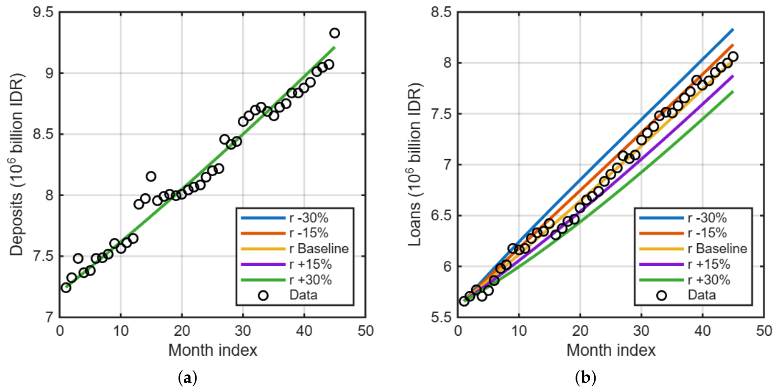
The reserve requirement parameter (r) is the proportion of deposits that must be kept as reserves and cannot be lent. Figure 2 shows that an increase in r reduces loans, but no change occurs in deposits. This is because an increase in r also decreases the amount of liquid assets available for loans.
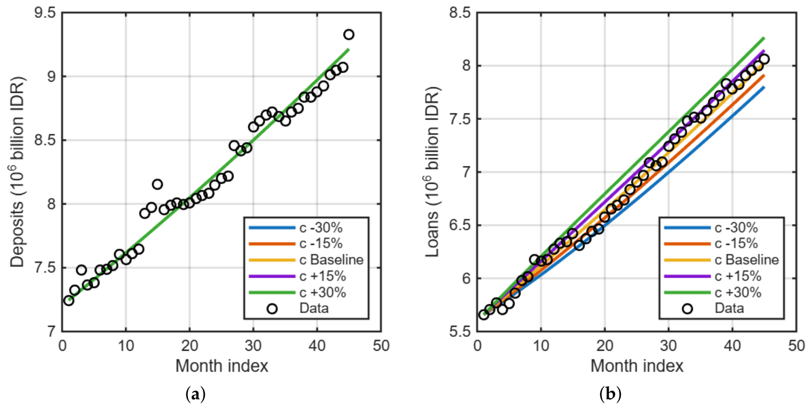
The capital adequacy ratio c is the minimum bank capital requirement per unit loan. Figure 3 shows that an increase in c results in higher loan levels, but no change occurs in deposits. An increase in the capital ratio leads to a greater term ( c + b 1 ) L and increases the liquidity. This helps to expand loans.

3. Optimal Control Model

In this section, an optimal control problem is formulated for the banking system model (4) and (5), where the reserve requirement ratio r ( t ) and the minimum capital adequacy ratio c ( t ) are treated as time-dependent regulatory control variables. These instruments are commonly used by banking regulators to indirectly influence banks’ liquidity and solvency conditions rather than directly controlling deposit and loan volumes.
The controlled state system is given by
d D d t = a D D 1 D K D w 0 D + ϕ A D ,
d L d t = a L A L 1 L K L η L δ ( 1 η ) L ,
where
A = ( 1 r ( t ) ) D + ( c ( t ) + b 1 ) L .
The regulator aims to maintain the bank loan-to-deposit ratio close to a prescribed target while simultaneously keeping the liquidity ratio near the desired benchmark. In addition, excessive regulatory intervention incurs implementation and compliance costs. The equations representing these objectives are as follows:
LDR ( t ) = L ( t ) D ( t ) , LR ( t ) = A ( t ) D ( t ) ,
where LDR ( t ) denotes the loan-to-deposit ratio, and LR ( t ) represents the liquidity ratio.
Let * > 0 denote the target loan-to-deposit ratio, κ * > 0 denote the target liquidity ratio set by the regulator, r 0 denote the reserve requirement policy rate, and c 0 denote the capital adequacy ratio policy rate. Then, the objective functional is defined by
J ( r , c ) = 0 T α L D * 2 + β A D κ * 2 + γ 1 ( r r 0 ) 2 + γ 2 ( c c 0 ) 2 d t ,
where α , β , γ 1 , γ 2 > 0 are the weight parameters. The first term within the integral penalizes deviations of the loan-to-deposit ratio from the target level ( * ); the second term penalizes deviations of the liquidity ratio from its desired benchmark ( κ * ); and the last two terms represent the costs associated with adjusting the reserve requirement and capital adequacy ratio requirement from the baseline policy rates, respectively.
The optimal control problem consists of finding measurable control functions r * ( t ) and c * ( t ) such that
J ( r * , c * ) = min ( r , c ) U J ( r , c ) ,
subject to the controlled state system (10)–(12) and the admissible control set
U = ( r , c ) : [ 0 , T ] R 2 | r min r ( t ) r max , c min c ( t ) c max , r , c measurable ,
where
0 < r min < r max < 1 , 0 < c min < c max < 1
are the prescribed bounds reflecting feasible regulatory ranges.
The regulator’s optimization problem is to determine the time paths of r ( t ) and c ( t ) that best stabilize the bank loan-to-deposit ratio and liquidity position while minimizing the cost of policy intervention.
To characterize the optimal reserve requirement ratio r ( t ) and minimum capital adequacy ratio c ( t ) , Pontryagin’s Maximum Principle was applied (Seierstad & Sydsaeter, 1986).
Let the state vector be x = ( D , L ) and the adjoint vector be λ = ( λ D , λ L ) .
Accordingly, the Hamiltonian is defined by
H ( D , L , r , c , λ D , λ L ) = α L D * 2 + β A D κ * 2 + γ 1 ( r r 0 ) 2 + γ 2 ( c c 0 ) 2 + λ D a D D 1 D K D w 0 D + ϕ A D + λ L a L A L 1 L K L θ L .
The existence of an optimal control pair is established.
Theorem 7.
Assume that the admissible control set U is nonempty and that c max + b < 1 and ϕ ( 1 r min ) < a D K D . Then, there exists an optimal control pair ( r * , c * ) U together with the corresponding state trajectory ( D * , L * ) minimizing the objective functional J ( r , c ) .
Proof. 
The set U in (14) is nonempty, closed, bounded, and convex in the space of bounded measurable control functions. For each ( r , c ) U , the right-hand side of the controlled state system is continuous in ( D , L ) and ( r , c ) and locally Lipschitz with respect to ( D , L ) . Therefore, for each admissible control pair ( r , c ) , the system admits a unique local solution.
Next, we show that ( D , L ) remains uniformly bounded for all admissible controls. Since c ( t ) + b 1 c max + b 1 < 0 and L ( t ) 0 , it follows that
A ( t ) ( 1 r min ) D ( t ) .
Under the assumptions c max + b < 1 and ϕ ( 1 r min ) < a D K D , the positivity and boundedness results established earlier in Section 2.2 remain valid for all admissible controls. Therefore, the corresponding state solutions ( D , L ) remain positive and are uniformly bounded. In particular, because D ( t ) > 0 and D is continuous on the compact interval [ 0 , T ] , the ratios L / D and A / D are well-defined and bounded for every admissible control pair ( r , c ) .
The integrand of J is continuous in the state variables and strictly convex in the controls ( r , c ) . Because the integrand is also bounded below by zero, all the standard hypotheses of the existence theorem for optimal controls are satisfied. According to the Filippov–Cesari existence theorem (Cesari, 2012; Filippov, 1962), there exists an optimal control pair ( r * , c * ) U with a corresponding optimal state trajectory ( D * , L * ) that minimizes J.    □
The necessary optimality conditions are as follows:
Theorem 8.
Let ( r * , c * ) U be an optimal control pair and ( D * , L * ) the corresponding optimal state trajectory of (10)–(12). Then there exists a nontrivial adjoint vector
λ ( t ) = λ D ( t ) , λ L ( t )
such that
λ ˙ D ( t ) = H D D * , L * , r * , c * , λ D , λ L , λ ˙ L ( t ) = H L D * , L * , r * , c * , λ D , λ L ,
with transversality conditions
λ D ( T ) = 0 , λ L ( T ) = 0 .
Moreover, the optimal controls r * ( t ) and c * ( t ) are characterized by
r * ( t ) = min max r ^ ( t ) , r min , r max ,
c * ( t ) = min max c ^ ( t ) , c min , c max ,
where ( r ^ ( t ) , c ^ ( t ) ) is the unconstrained minimizer of the Hamiltonian, obtained from the linear system
γ 1 + β β z * β z * γ 2 + β ( z * ) 2 r ^ c ^ = β χ * + γ 1 r 0 + N r * 2 β z * χ * + γ 2 c 0 N c * 2 ,
with
z * = L * D * , χ * = 1 + ( b 1 ) L * D * κ * ,
and
N r * = ϕ λ D ( D * ) 2 + a L λ L D * L * 1 L * K L , N c * = ϕ λ D D * L * + a L λ L ( L * ) 2 1 L * K L .
Equivalently, since
= ( γ 1 + β ) γ 2 + β ( z * ) 2 β 2 ( z * ) 2 = γ 1 γ 2 + β γ 2 + β γ 1 ( z * ) 2 > 0 ,
the unconstrained controls are explicitly given by
r ^ ( t ) = γ 2 + β ( z * ) 2 2 β χ * + 2 γ 1 r 0 + N r * + β z * 2 β z * χ * + 2 γ 2 c 0 N c * 2 ,
c ^ ( t ) = β z * 2 β χ * + 2 γ 1 r 0 + N r * + ( γ 1 + β ) 2 β z * χ * + 2 γ 2 c 0 N c * 2 .
Proof. 
By Theorem 7, an optimal control pair ( r * , c * ) U exists. Since the admissible control set U is convex and the state equations are continuously differentiable with respect to the state variables ( D , L ) and control variables ( r , c ) , Pontryagin’s Maximum Principle applies. Hence, there exists a nontrivial adjoint vector ( λ D , λ L ) satisfying the adjoint system (16) together with the transversality conditions
λ D ( T ) = 0 , λ L ( T ) = 0 .
The optimality condition requires that the optimal controls minimize the Hamiltonian. Therefore,
H r = 0 , H c = 0 .
Using
A = ( 1 r ) D + ( c + b 1 ) L , A r = D , A c = L ,
and defining
z = L D , χ = 1 + ( b 1 ) L D κ * ,
yields
H r = 2 β χ r + c z + 2 γ 1 ( r r 0 ) ϕ λ D D 2 a L λ L D L 1 L K L , H c = 2 β z χ r + c z + 2 γ 2 ( c c 0 ) + ϕ λ D D L + a L λ L L 2 1 L K L .
Setting these derivatives to zero yields the linear system in (19). The coefficient matrix
M = γ 1 + β β z β z γ 2 + β z 2 .
has determinant
= γ 1 γ 2 + β γ 2 + β γ 1 z 2 > 0 ,
Therefore, the system (19) has a unique solution, namely, (20) and (21). Finally, considering the admissible bounds on the controls
r min r ( t ) r max , c min c ( t ) c max ,
the optimal controls are obtained by projecting onto the control set, which gives (17) and (18).    □

Numerical Simulations

This subsection presents the numerical simulations of the optimal control problem. The objective is to regulate the reserve requirement r ( t ) and capital adequacy ratio c ( t ) to stabilize the loan-to-deposit ratio (LDR) and liquidity ratio (LR) around the desired targets while minimizing the cost of intervention. In our simulation, we used the LDR target bound: 84–94% (Bank Indonesia, 2018). By this target, then from the balance sheet identity we have
A = ( 1 r ) D + ( c + b 1 ) L A D = 1 r + ( c + b 1 ) L D .
Using the parameter values from Table 1 of r = 9 % , c = 8 % , b = 16.73 % , and the LDR target bound of 84 % L D 94 % , we determine the LR target bound as 20 % A D 28 % . For the policy target bounds for r ( t ) and c ( t ) , we employed the same bounds as those used in the sensitivity analysis in Section 2.6, that is ( 1 30 % ) 9 % r ( t ) ( 1 + 30 % ) 9 % and ( 1 30 % ) 8 % c ( t ) ( 1 + 30 % ) 8 % .
For simulation purposes, we set the control target: * = 89 % (midpoint of LDR target bound), κ * = 24 % (midpoint of LR target bound), r 0 = 9 % (reserve requirement policy), and c 0 = 8 % (capital adequacy ratio policy). We use time horizon [ 0 , 250 ] and initial values D ( 0 ) = 7.244982711 and L ( 0 ) = 5.657604888 .
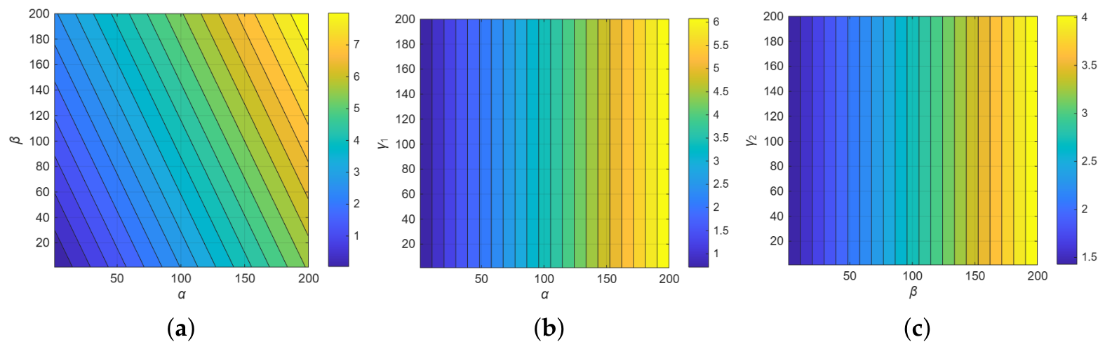
As for the weight parameters of the objective function J, specifically α , β , γ 1 , and γ 2 , we do not have specific values. However, as an illustration, Figure 4 presents a simulated contour plot of J with varying parameters α , β , γ 1 , and γ 2 ranging from 1 to 200. In Figure 4a,b, we can observe that the parameter α contributes more significantly to J than the parameters β and γ 1 , whereas β contributes more significantly than γ 2 . This implies that the objective function is more sensitive to the weight assigned to the LDR target than to the other weights.
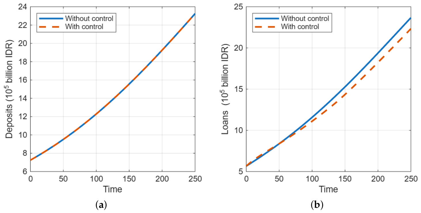
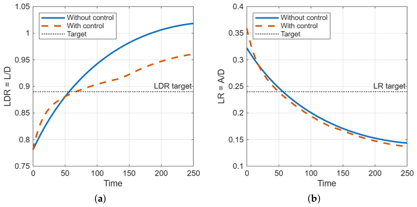
In Figure 5, we compare the time evolution of deposits and loans with and without the optimal control. In this simulation, for illustrative purposes, we set α = β = γ 1 = γ 2 = 50 . These parameter values are chosen for simplicity. We observe that the controlled system leads to lower levels of loans, but nothing happens to the deposits.
In contrast, Figure 6 shows the dynamics of the loan-to-deposit ratio (LDR) and liquidity ratio (LR). With optimal control, the LDR was significantly lower and closer to the target LDR level than that in the uncontrolled system. However, the LR is slightly lower than that of the uncontrolled case. These findings show that the control approach has a stabilizing impact on the LDR as a key financial ratio of the banking system.
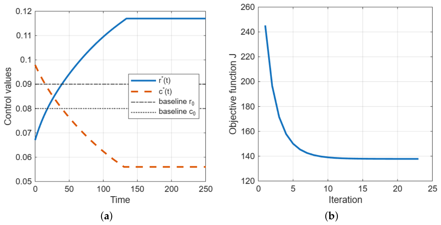
The trajectories of the optimal control variables ( r * ( t ) , c * ( t ) ) are shown in Figure 7a. The reserve requirement r * ( t ) increases transiently, followed by a convergence to an optimal value r * = 11.7 % . On the other hand, the capital adequacy ratio c * ( t ) increases transiently, followed by a convergence to an optimal value r * = 5.6 % .
In Figure 7b, we report the dynamics of the objective function during the optimization process. The continuous decline in the objective function suggests convergence of the numerical solution and success of the optimization process.

4. Stochastic Model

In reality, the banking business is subject to random variations due to market dynamics, depositor behavior, and credit risk. Deposit withdrawals and loan performance are influenced by external factors that change over time. For instance, depositor sentiment, market expectations, and trust in the banking sector can lead to unexpected shifts in withdrawal patterns (Dragomirescu-Gaina et al., 2024; Ferreira & Dickason-Koekemoer, 2020; Rashid et al., 2024). Similarly, macroeconomic conditions such as inflation, interest rate changes, and unemployment can impact borrowers’ ability to repay loans, thereby affecting non-performing loan rates (Annas et al., 2024; Syed & Tripathi, 2019; Viphindrartin et al., 2021).
From a modeling perspective, the proposed deterministic model captures only the typical behavior of banking variables, overlooking random variations from the deterministic trajectory. Stochastic differential equations offer a suitable framework for integrating these uncertainties by permitting key parameters to vary randomly around their average values. This allows for the exploration of not only the anticipated progression of deposits and loans but also the system’s variability under uncertain conditions. Driven by these factors, we extend the deterministic model to a stochastic differential equation system where withdrawal and non-performing loan rates experience random shocks.
This study assumes that the baseline withdrawal rate w 0 and the non-performing loan rate η are affected by environmental noise. The model is formally introduced as follows.
w 0 w 0 + σ 1 B ˙ 1 ( t ) , η η + σ 2 B ˙ 2 ( t ) ,
where B 1 ( t ) and B 2 ( t ) are independent standard Brownian motions, and σ 1 , σ 2 > 0 denote the noise intensities associated with withdrawal and credit-risk shocks, respectively.
Substituting these perturbations into system (4) and (5), the stochastic model results in Itô form:
d D t = a D D t 1 D t K D w 0 D t + ϕ A t D t d t σ 1 D t d B 1 ( t ) ,
d L t = a L A t L t 1 L t K L η L t δ ( 1 η ) L t d t + σ 2 ( δ 1 ) L t d B 2 ( t ) ,
where
A t = ( 1 r ) D t + ( c + b 1 ) L t .
The diffusion term in (22) follows from the evidence that the uncertainty in the withdrawal parameter directly affects the deposit-loss term w 0 D t . Similarly, since the loan equation contains the term η L t δ ( 1 η ) L t = η ( δ 1 ) δ L t , random perturbation of η yields the diffusion coefficient σ 2 ( δ 1 ) L t .
The parameter σ 1 measures the magnitude of exogenous liquidity shocks affecting deposits, whereas σ 2 quantifies the volatility of loan quality shocks affecting the loan portfolio.
For the numerical simulation, the system in (22) and (23) was discretized using the Euler–Maruyama method (Higham, 2001). Let t n = n t , D n D ( t n ) , and L n L ( t n ) . Then
D n + 1 = D n + a D D n 1 D n K D w 0 D n + ϕ A n D n t σ 1 D n B 1 , n ,
L n + 1 = L n + a L A n L n 1 L n K L η L n δ ( 1 η ) L n t + σ 2 ( δ 1 ) L n B 2 , n ,
where
A n = ( 1 r ) D n + ( c + b 1 ) L n ,
and
B 1 , n , B 2 , n N ( 0 , t )
is an independent Gaussian increment.

Numerical Scheme

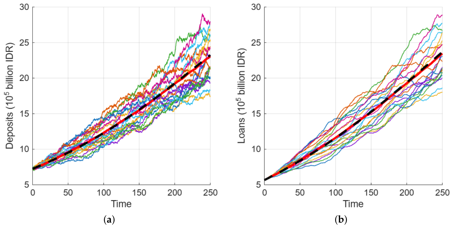
This subsection investigates the impact of stochastic fluctuations on deposit and loan dynamics. The stochastic model in (22) and (23) was simulated using the Euler–Maruyama method. A total of M = 200 sample paths were generated to capture the variability induced by randomness. The noise intensities σ 1 and σ 2 are determined as follows. In Table 1, η ( t ) represents a time series of the training data, whose mean and standard deviation are η = 2.61 % and σ 2 = 0.31 % , respectively. However, time-series data are lacking for the withdrawal scenario. Therefore, we set w 0 = 6.37 × 10 6 as shown in Table 1, and σ 1 is estimated from the standard deviation of the relative change in deposit data, D ( t + 1 ) D ( t ) D ( t ) . This yields σ 1 = 1.08 % .
We show multiple sample trajectories of deposits and loans under stochastic perturbations in Figure 8. It is apparent that both variables fluctuate considerably around their deterministic solutions. The variability increases over time as stochastic shocks accumulate. The deterministic trend in growth remains, suggesting that the system is not sensitive to moderate levels of noise.
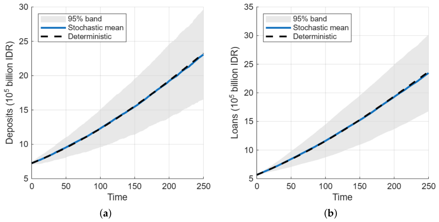
In Figure 9, we plot the mean and the 95 % confidence intervals of the stochastic solution alongside the deterministic one. The stochastic mean closely aligns with the deterministic solution for both deposits and loans, indicating that the deterministic model captures the expected dynamics of the system well. However, the confidence bounds grow over time, suggesting that the uncertainty of the system increases with time and that stochastic effects should be considered when making long-term predictions.
Specifically, the uncertainty around deposits is slightly greater than that around loans, reflecting the direct influence of withdrawal shocks on deposit dynamics. In contrast, loan dynamics are indirectly influenced by both liquidity requirements and stochastic shocks to the non-performing loan rate.

5. Conclusions

In this study, we propose a mathematical model of banking dynamics that consists of three components: a deterministic nonlinear system, an extended optimal control system, and a stochastic system. The deterministic model describes the interplay between deposits and loans via liquidity effects and regulatory requirements, with liquid assets affecting both deposit dynamics and loan growth. The optimal control model incorporates regulatory controls, such as reserve requirements and capital adequacy ratios, to stabilize certain financial ratios, such as the loan-to-deposit and liquidity ratios. The deterministic model is then extended to a stochastic model that accounts for randomness in withdrawals and non-performing loans to capture uncertainty in banking dynamics.
Theoretically, we ensured the well-posedness of the deterministic system through positivity and boundedness of solutions and detected mathematical equilibria (trivial and boundary equilibria) and economically admissible equilibria (interior equilibria) with clear conditions. We found that the local stability of economically admissible equilibria is controlled by the trace and determinant of the linearized system. The estimation of parameters using Indonesian bank data via particle swarm optimization resulted in a low MAPE, validating the model’s capability to fit real banking data. The proposed model also has a slightly lower MAPE than the benchmark model while maintaining comparable directional forecasting performance. Sensitivity analysis also shows that increased capital adequacy ratios facilitate loan growth lending, while reserve requirements hinder loan growth. In the empirical banking literature, stricter capital requirements may reduce lending through balance sheet constraints. Therefore, the positive effect observed here should be interpreted as a liquidity confidence channel specific to the proposed framework rather than a universal regulatory outcome.
The optimal control results show that the time-varying regulation of the reserve requirement and capital adequacy ratio produces lower loan growth, but with an LDR closer to the target with relatively low control costs. Furthermore, the stochastic version demonstrated that while uncertainty in withdrawals and non-performing loans adds volatility, the mean path of the stochastic solution is consistent with the deterministic model, suggesting that the stochastic model is robust to data-based moderate randomness and captures increasing variability over time.
From a practical perspective, the proposed model, calibrated with Indonesian banking data, can serve as a tool for regulators and bank managers to evaluate the implications of regulatory policy changes, devise strategies that balance lending activities with liquidity resilience, and support reliable forecasting of banking dynamics under uncertain economic conditions.
The model presented in this study considers equity as a constant fraction of loans, which simplifies the models and facilitates the analysis. However, this assumption neglects the dynamic evolution of equity resulting from retained earnings, losses, dividends, and capital injections. Therefore, the model may not fully capture changes in a bank’s capital position during periods of significant profitability or financial distress. Therefore, future research could relax this assumption by modeling equity as a dynamic state variable driven by banks’ profits and losses, following the approach in Ansori et al. (2025). Other possible extensions include a two-bank model, an interbank network, incorporating macroeconomic variables, or addressing systemic risk and policies.

Author Contributions

M.F.A.: Conceptualization, Methodology, Software, Formal analysis, Investigation, Writing—Original Draft, Writing—Review and Editing, Funding acquisition; F.H.G.: Formal analysis, Investigation, Writing—Original Draft, Writing—Review and Editing; R.H.: Project administration, Writing—Original Draft, Writing—Review and Editing, Funding acquisition; H.K.F.: Writing—Original Draft, Writing—Review and Editing, Funding acquisition; N.Y.A.: Writing—Original Draft, Writing—Review and Editing, Funding acquisition; H.L.S.: Writing—Original Draft, Writing—Review and Editing, Funding acquisition. All authors have read and agreed to the published version of the manuscript.

Funding

This study was supported by Dana Selain APBN Faculty of Science and Mathematics, Universitas Diponegoro, through the research grant “Riset Kompetisi FSM Undip 2026” with contract no. 451.N/UN7.F8/PP/III/2026.

Institutional Review Board Statement

Not applicable.

Informed Consent Statement

Not applicable.

Data Availability Statement

The data used in this study are publicly available from the official website of the Indonesian Financial Service Authority (Otoritas Jasa Keuangan—OJK) at URL (accessed on 1 May 2026) https://www.ojk.go.id/id/kanal/perbankan/data-dan-statistik/statistik-perbankan-indonesia/Default.aspx. The MATLAB R2026a codes used for parameter estimation using PSO, sensitivity simulations, optimal control model computation, and stochastic model simulations are available from the corresponding author upon reasonable request.

Conflicts of Interest

The authors declare no conflicts of interest.

References

  1. Abdukadyrova, G., Tabyshova, A., Nazekova, M., Alymbaeva, J., & Toktosunova, C. (2024). Comprehensive dynamics of banking: A systemic approach incorporating lending, investment, and capital variables. Journal of Systems Science and Information, 12(3), 323–339. [Google Scholar] [CrossRef]
  2. Acharya, V., Almeida, H., Ippolito, F., & Orive, A. P. (2020). Bank lines of credit as contingent liquidity: Covenant violations and their implications. Journal of Financial Intermediation, 44, 100817. [Google Scholar] [CrossRef]
  3. Adebisi, O. O., Love, M. C., & Emena, O. U. (2018). Corporate governance mechanisms and asset quality: The case of non-performing loans in Nigerian deposit money banks. In K. S. Soliman (Ed.), 31st international business information management association conference, IBIMA 2018: Innovation management and education excellence through vision 2020 (pp. 5070–5085). International Business Information Management Association, IBIMA. [Google Scholar]
  4. Ally, O. J., Kulindwa, Y. J., & Mataba, L. (2025). Financial technology and credit risk management: The case of non-performing loans in Tanzanian banks. Cogent Economics and Finance, 13(1), 2459188. [Google Scholar] [CrossRef]
  5. Al-Shimmery, A. A. A. J. (2019). Bank deposits and their impact on supporting the financial stability of banks. Opcion, 35(20), 499–515. [Google Scholar]
  6. Annas, M., Humairoh, H., & Endri, E. (2024). Macroeconomic and bank-specific factors on non-performing loan: Evidence from an emerging economy. Quality—Access to Success, 25(199), 155–161. [Google Scholar] [CrossRef]
  7. Ansori, M. F. (2026). Dynamic modeling and optimal control of bank balance sheets under capital adequacy constraints. An International Journal of Optimization and Control: Theories & Applications, 16(1), 40–53. [Google Scholar] [CrossRef]
  8. Ansori, M. F., Ashar, N. Y., & Fata, H. K. (2025). Logistic map-based banking loan dynamics with central bank policies. Journal of Applied Nonlinear Dynamics, 14(3), 561–574. [Google Scholar] [CrossRef]
  9. Ansori, M. F., Brianzoni, S., & Campisi, G. (2024). Bifurcations and complex dynamics in a banking duopoly model with macroprudential policy. Physica A: Statistical Mechanics and Its Applications, 641, 129730. [Google Scholar] [CrossRef]
  10. Ansori, M. F., & Hariyanto, S. (2022). Analysis of banking deposit cost in the dynamics of loan: Bifurcation and chaos perspectives. Barekeng, 16(4), 1283–1292. [Google Scholar] [CrossRef]
  11. Ansori, M. F., & Khabibah, S. (2022). The role of cost of loan in banking loan dynamics: Bifurcation and chaos analysis. Barekeng, 16(3), 1031–1038. [Google Scholar] [CrossRef]
  12. Ansori, M. F., Sumarti, N., Sidarto, K. A., & Gunadi, I. (2021). An algorithm for simulating the banking network system and its application for analyzing macroprudential policy. Computer Research and Modeling, 13(6), 1275–1289. [Google Scholar] [CrossRef]
  13. Ansori, M. F., Sumarti, N., Sidarto, K. A., Gunadi, I., & Gümüş, F. H. (2025). Mathematical model of bank balance sheet with a macroprudential instrument and its application to banking data. Mathematical Methods in the Applied Sciences, 48(18), 16789–16803. [Google Scholar] [CrossRef]
  14. Antonio, Y., Ansori, M. F., Shavera, S., Avrila, N., Sasmito, A., & Nisa, H. (2025). A scale-free interbank connection network for banking systemic risk modeling. In 2025 international conference on computer and applications (ICCA) (pp. 1–6). IEEE. [Google Scholar] [CrossRef]
  15. Ábel, I., & Mérő, K. (2023). Endogenous money, soft budget constraint and the banking regulation. Acta Oeconomica, 73, 99–118. [Google Scholar] [CrossRef]
  16. Bank Indonesia. (2018). Bank Indonesia regulation no. 20/4/PBI/2018 on macroprudential intermediation ratio and macroprudential liquidity buffer for conventional commercial banks, islamic commercial banks, and islamic business units. Bank Indonesia. (Original title in Indonesian: Peraturan bank Indonesia nomor 20/4/PBI/2018 tentang rasio intermediasi makroprudensial dan penyangga likuiditas makroprudensial bagi bank umum konvensional, bank umum syariah, dan unit usaha syariah).
  17. Bank Indonesia. (2022). Board of governors regulation no. 24/8/PADG/2022 on minimum reserve requirements in rupiah for conventional commercial banks. Bank Indonesia. (Original title in Indonesian: Peraturan anggota dewan gubernur nomor 24/8/PADG/2022 tentang peraturan pelaksanaan pemenuhan giro wajib minimum dalam rupiah dan valuta asing bagi bank umum konvensional, bank umum syariah, dan unit usaha syariah). Available online: https://www.bi.go.id/id/publikasi/peraturan/Pages/PADG_240822.aspx (accessed on 25 April 2026).
  18. Bauso, D., Odijk, M., & Ramirez, S. (2026). Cascading failures in financial networks: Dynamics, stability, and control. IEEE Transactions on Automatic Control, 71(3), 1724–1736. [Google Scholar] [CrossRef]
  19. Bleck, A., & Liu, X. (2018). Credit expansion and credit misallocation. Journal of Monetary Economics, 94, 27–40. [Google Scholar] [CrossRef]
  20. Boamah, N. A., Opoku, E., & Boakye-Dankwa, A. (2023). Capital regulation, liquidity risk, efficiency and banks performance in emerging economies. Journal of Financial Regulation and Compliance, 31(1), 126–145. [Google Scholar] [CrossRef]
  21. Bozhalkina, Y. (2017). Mathematical model of the loan portfolio dynamics in the form of Markov chain considering the process of new customers attraction. AIP Conference Proceedings, 1910, 020009. [Google Scholar] [CrossRef]
  22. Bräuning, F., & Fecht, F. (2017). Relationship lending in the interbank market and the price of liquidity. Review of Finance, 21(1), 33–75. [Google Scholar] [CrossRef]
  23. Cappelletti, G., & Mistrulli, P. E. (2023). The role of credit lines and multiple lending in financial contagion and systemic events. Journal of Financial Stability, 67, 101141. [Google Scholar] [CrossRef]
  24. Carletti, E., De Marco, F., Ioannidou, V., & Sette, E. (2021). Banks as patient lenders: Evidence from a tax reform. Journal of Financial Economics, 141(1), 6–26. [Google Scholar] [CrossRef]
  25. Cesari, L. (2012). Optimization theory and applications: Problems with ordinary differential equations. Springer Science & Business Media. [Google Scholar]
  26. Chand, S. A., Kumar, R. R., & Stauvermann, P. J. (2024). Determinants of bank deposit in a small economy’s banking sector: A study of Fiji. Accounting Research Journal, 37(6), 574–594. [Google Scholar] [CrossRef]
  27. Chauhan, R., & Sharma, A. K. (2025). The effect of liquidity creation on bank profitability and credit risk: Evidence from BRICS countries. Afro-Asian Journal of Finance and Accounting, 15(1), 19–40. [Google Scholar] [CrossRef]
  28. Chawwa, T. (2021). Impact of reserve requirement and liquidity coverage ratio: A DSGE model for Indonesia. Economic Analysis and Policy, 71, 321–341. [Google Scholar] [CrossRef]
  29. Cocco, J. F., Gomes, F. J., & Martins, N. C. (2009). Lending relationships in the interbank market. Journal of Financial Intermediation, 18(1), 24–48. [Google Scholar] [CrossRef]
  30. Costa, S., Faias, M., Júdice, P., & Mota, P. (2021). Panel data modeling of bank deposits. Annals of Finance, 17(2), 247–264. [Google Scholar] [CrossRef]
  31. De Haas, R., & Van Lelyveld, I. (2014). Multinational banks and the global financial crisis: Weathering the perfect storm? Journal of Money, Credit and Banking, 46(Suppl. S1), 333–364. [Google Scholar] [CrossRef]
  32. De Moraes, C. O., Gutierrez, M., & Barbosa, R. (2015). The aggregate behavior of banks: A proposal for prudential supervision. Latin American Business Review, 16(2), 87–101. [Google Scholar] [CrossRef]
  33. Diamond, D. W., & Dybvig, P. H. (1983). Bank runs, deposit insurance, and liquidity. Journal of Political Economy, 91(3), 401–419. [Google Scholar] [CrossRef]
  34. Dombret, A. R., Foos, D., Pliszka, K., & Schulz, A. (2019). What are the real effects of financial market liquidity? Evidence on bank lending from the euro area. Journal of International Financial Markets, Institutions and Money, 62, 152–183. [Google Scholar] [CrossRef]
  35. Dragomirescu-Gaina, C., Monticini, A., & Salsano, F. (2024). Media news and market expectations: Insights into the ECB’s new data-dependent policy regime. Economics Letters, 244, 111987. [Google Scholar] [CrossRef]
  36. Dutto Giolongo, M. L., & Carlevaro, E. A. (2019). Liquidity provision on demand in the argentine banking system. Emerging Markets Finance and Trade, 55(3), 634–654. [Google Scholar] [CrossRef]
  37. Fatone, L., & Mariani, F. (2020). Systemic risk governance in a dynamical model of a banking system with stochastic assets and liabilities. Journal of Economic Interaction and Coordination, 15(1), 183–219. [Google Scholar] [CrossRef]
  38. Ferreira, S. J., & Dickason-Koekemoer, Z. (2020). The influence of behavioural finance biases on depositor behaviour. International Journal of Business and Management Science, 10(1), 67–82. [Google Scholar]
  39. Filippov, A. F. (1962). On certain questions in the theory of optimal control. Journal of the Society for Industrial and Applied Mathematics, Series A: Control, 1(1), 76–84. [Google Scholar] [CrossRef] [PubMed]
  40. Gao, Q., Fan, H., & Pang, C. (2025). Monetary policy and systemic risk in a financial network system based on multi-agent modeling. Mathematics, 13(3), 378. [Google Scholar] [CrossRef]
  41. Gunay, S. (2020). Seeking causality between liquidity risk and credit risk: TED-OIS spreads and CDS indexes. Research in International Business and Finance, 52, 101189. [Google Scholar] [CrossRef]
  42. Gümüş, F. H., & Ansori, M. F. (2026). Adaptive dynamics of bank lending under credit risk: A discrete-time modeling approach. Konuralp Journal of Mathematics, 14(1), 87–98. [Google Scholar]
  43. Higham, D. J. (2001). An algorithmic introduction to numerical simulation of stochastic differential equations. SIAM Review, 43(3), 525–546. [Google Scholar] [CrossRef]
  44. Hodula, M., Komárková, Z., & Pfeifer, L. (2021). The relationship between capital and liquidity prudential instruments. Journal of Regulatory Economics, 59(1), 47–70. [Google Scholar] [CrossRef]
  45. Hossain, B., Bhuiyan, M. A. H., & Rahman, H. (2013). Deposit behavior and its impact on loan: A case study on rajshahi krishi unnayan bank (Rakub), Bangladesh. Journal of Economic Cooperation and Development, 34(4), 47–59. [Google Scholar]
  46. Huynh, J. (2025). Monetary policy interest rates and bank risk-return tradeoff: How does bank competition moderate this relationship? Bulletin of Monetary Economics and Banking, 28(2), 173–197. [Google Scholar] [CrossRef]
  47. Jung, H., & Kim, D. (2015). Bank funding structure and lending under liquidity shocks: Evidence from Korea. Pacific Basin Finance Journal, 33, 62–80. [Google Scholar] [CrossRef]
  48. Kashyap, A. K., Rajan, R., & Stein, J. C. (2002). Banks as liquidity providers: An explanation for the coexistence of lending and deposit-taking. Journal of Finance, 57(1), 33–73. [Google Scholar] [CrossRef]
  49. Košak, M., Li, S., Lončarski, I., & Marinč, M. (2015). Quality of bank capital and bank lending behavior during the global financial crisis. International Review of Financial Analysis, 37, 168–183. [Google Scholar] [CrossRef]
  50. Lampart, M., Lampartová, A., & Orlando, G. (2023). On risk and market sentiments driving financial share price dynamics. Nonlinear Dynamics, 111, 16585–16604. [Google Scholar] [CrossRef]
  51. Leroy, A., & Lucotte, Y. (2015). Heterogeneous monetary transmission process in the Eurozone: Does banking competition matter? International Economics, 141, 115–134. [Google Scholar] [CrossRef]
  52. Ling, D. X., Haron, R., & Hasan, A. (2022). Basel III capital regulation framework and Islamic bank’s risk. IIUM Law Journal, 30(S2), 93–128. [Google Scholar] [CrossRef]
  53. Liu, G., Liu, H., He, F., & Li, Y. (2025). Banks’ liability structure and monetary policy transmission: Evidence from a quasi-natural experiment in China. European Journal of Finance, 31(17), 2145–2167. [Google Scholar] [CrossRef]
  54. Mallett, J. (2012). What are the limits on commercial bank lending? Advances in Complex Systems, 15(Suppl. S2), 1250075. [Google Scholar] [CrossRef]
  55. M’bakob, G. B., & Tchounga, A. (2024). CBDC and banking stability: Modeling cascading effects on reserves, lending, and liquidity. Research in Economics, 78(4), 101005. [Google Scholar] [CrossRef]
  56. Mohammed, S. A. S. A. (2025). Corruption, non-performing loans, and financial innovation: The role of fintech and bank regulations in emerging markets. Macroeconomics and Finance in Emerging Market Economies. [Google Scholar] [CrossRef]
  57. Neamah, Z. H., Alawsi, A. A. M., Ali, H. M., Ali, A. M. A., & Al-Baghdadi, A. F. (2025). Novel 3D-chaotic financial model with mesh attractor: Complexity analysis. Mathematics for Applications, 14(1), 105–112. [Google Scholar] [CrossRef]
  58. Neziraj Elshani, A. (2025). Impact of non-performing loans on deposits and financial stability: An empirical analysis in developing european countries. Journal of Risk Analysis and Crisis Response, 15(3), 622–639. [Google Scholar] [CrossRef]
  59. Orlando, G., & Bufalo, M. (2021). Interest rates forecasting: Between hull and white and the CIR#—How to make a single-factor model work. Journal of Forecasting, 40(8), 1566–1580. [Google Scholar] [CrossRef]
  60. Otoritas Jasa Keuangan. (2016). Indonesian financial services authority regulation no. 11/POJK.03/2016 on minimum capital adequacy requirements for commercial banks. Otoritas Jasa Keuangan. (Original title in Indonesian: Peraturan otoritas jasa keuangan nomor 11 /POJK.03/2016 tentang kewajiban penyediaan modal minimum bank umum). Available online: https://www.ojk.go.id/id/kanal/perbankan/regulasi/peraturan-ojk/Documents/Pages/pojk11-kewajiban-penyediaan-modal-minimum-bank-umum/SALINAN-POJK.11%20Konversi%20KPMM%20FINALE.pdf (accessed on 25 April 2026).
  61. Otoritas Jasa Keuangan. (2021). Indonesian financial services authority regulation no. 12/POJK.03/2021 on commercial banks. Otoritas Jasa Keuangan. (Original title in Indonesian: Peraturan otoritas jasa keuangan (POJK) nomor 12/POJK.03/2021 tentang bank umum).
  62. Otoritas Jasa Keuangan. (2025). Indonesia banking statistics (Statistik perbankan Indonesia). (Monthly publication providing statistical data on the Indonesian banking sector). Available online: https://ojk.go.id/id/kanal/perbankan/data-dan-statistik/statistik-perbankan-indonesia/Default.aspx (accessed on 1 May 2026).
  63. Pedrosa, A. B., & Mansilla Fernández, J. M. (2020). Unconventional monetary policy, competition and financial stability. Evidence from the eurozone banks. Estudios de Economia Aplicada, 38(1), 1–18. [Google Scholar] [CrossRef]
  64. Qiu, J. (2011). Bank money, aggregate liquidity, and asset prices. Annals of Economics and Finance, 12(2), 295–346. [Google Scholar]
  65. Rashid, N., Azam, A. H. M., Sarmidi, T., & Radzi, N. A. M. (2024). Asymmetric effect of market sentiment on banking: A nonlinear ARDL approach; [Kesan asimetri sentimen pasaran terhadap perbankan: Pendekatan ARDL tidak linear]. Jurnal Ekonomi Malaysia, 58(2), 104–119. [Google Scholar] [CrossRef]
  66. Ritz, R. A., & Walther, A. (2015). How do banks respond to increased funding uncertainty? Journal of Financial Intermediation, 24(3), 386–410. [Google Scholar] [CrossRef]
  67. Rumiantsev, M. (2008). Simulation modeling of financial-crediting institution activities by means of system dynamics. Actual Problems of Economics, 86, 230–239. [Google Scholar]
  68. Segev, N., & Schaffer, M. (2020). Monetary policy, bank competition and regional credit cycles: Evidence from a quasi-natural experiment. Journal of Corporate Finance, 64, 101494. [Google Scholar] [CrossRef]
  69. Seierstad, A., & Sydsaeter, K. (1986). Optimal control theory with economic applications. Elsevier North-Holland, Inc. [Google Scholar]
  70. Sharma, V. (2026). Lending relationships and boom-bust cycles. Journal of Financial Stability, 83, 101511. [Google Scholar] [CrossRef]
  71. Shikimi, M. (2023). Risk-taking and bank competition under a low interest rate environment: Evidence from loan-level data. Pacific Basin Finance Journal, 78, 101945. [Google Scholar] [CrossRef]
  72. Song, F., & Thakor, A. V. (2007). Relationship banking, fragility, and the asset-liability matching problem. Review of Financial Studies, 20(6), 2129–2177. [Google Scholar] [CrossRef]
  73. Syed, A. A., & Tripathi, R. (2019). Non-performing loans in BRICS nations: Determinants and macroeconomic impact. Indian Journal of Finance, 13(2), 22–35. [Google Scholar] [CrossRef]
  74. Talavera, O., Tsapin, A., & Zholud, O. (2012). Macroeconomic uncertainty and bank lending: The case of Ukraine. Economic Systems, 36(2), 279–293. [Google Scholar] [CrossRef]
  75. Temizsoy, A., Iori, G., & Montes-Rojas, G. (2015). The role of bank relationships in the interbank market. Journal of Economic Dynamics and Control, 59, 118–141. [Google Scholar] [CrossRef]
  76. Timofeeva, G., Bozhalkina, Y., & Timofeev, N. (2018). Loan portfolio payment flows management considering macroeconomic parameters forecast. AIP Conference Proceedings, 2025(1), 040015. [Google Scholar] [CrossRef]
  77. Tran, D. V. (2020). Funding liquidity and bank lending. Cogent Economics and Finance, 8(1), 1734324. [Google Scholar] [CrossRef]
  78. Tran, H. S., Nguyen, T. D., & Nguyen, T. L. (2023). Market structure, institutional quality and bank stability: Evidence from emerging and developing countries. Competitiveness Review, 33(6), 1046–1068. [Google Scholar] [CrossRef]
  79. van Leuvensteijn, M., Kok Sørensen, C., Bikker, J. A., & van Rixtel, A. R. J. M. (2013). Impact of bank competition on the interest rate pass-through in the euro area. Applied Economics, 45(11), 1359–1380. [Google Scholar] [CrossRef]
  80. Viphindrartin, S., Ardhanari, M., Wilantari, R. N., Somaji, R. P., & Arianti, S. (2021). Effects of bank macroeconomic indicators on the stability of the financial system in Indonesia. Journal of Asian Finance, Economics and Business, 8(1), 647–654. [Google Scholar] [CrossRef]
  81. Zakharov, K., Kovantsev, A., & Boukhanovsky, A. (2025). A dynamic model of customers behavior: Integrating econophysics and physics-informed neural networks. In M. H. Lees, W. Cai, S. A. Cheong, Y. Su, D. Abramson, J. J. Dongarra, & P. M. Sloot (Eds.), Computational science—ICCS 2025 (Vol. 15903, pp. 238–252). Springer. [Google Scholar] [CrossRef]
  82. Zhang, X., Tan, W., Yu, M., Huangpeng, Q., & Duan, X. (2026). Interaction modeling and system stability analysis in financial markets. In S. Kovalev, I. Kotenko, & A. Sukhanov (Eds.), Proceedings of the ninth international scientific conference “intelligent information technologies for industry” (IITI’25), volume 1 (Vol. 1762, pp. 623–633). Springer. [Google Scholar] [CrossRef]
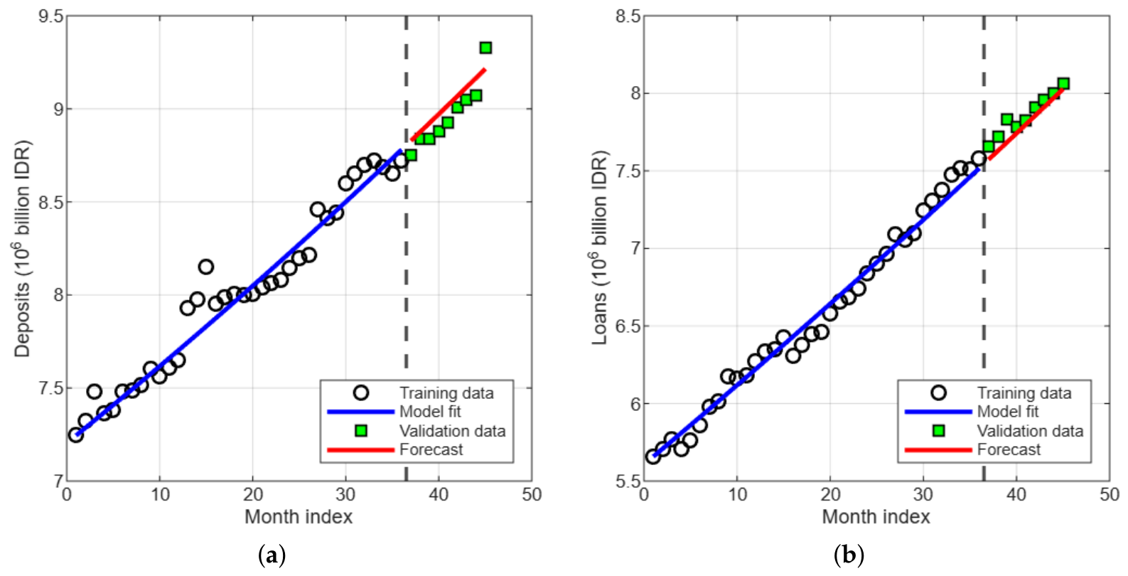
Figure 1. Comparison between observed Indonesian bank data and the proposed model (4) and (5) simulation using parameter values in Table 1. (a) Model fit for deposits. (b) Model fit for loans.
Ijfs 14 00174 g001
Figure 2. Sensitivity of deposits and loans with respect to reserve requirement policy rate r perturbed by 30 % , 15 % , 0 % (baseline), + 15 % , and + 30 % relative to its policy rate. (a) Deposits for varying r. (b) Loans for varying r.
Ijfs 14 00174 g002
Figure 3. Sensitivity of deposits and loans with capital adequacy ratio policy rate c perturbed by 30 % , 15 % , 0 % (baseline), + 15 % , and + 30 % relative to its policy rate. (a) Deposits for varying c. (b) Loans for varying c.
Ijfs 14 00174 g003
Figure 4. Contour plot of the objective function J when the weights parameters α , β , γ 1 , and γ 2 vary ranging from 1 to 200. (a) α and β vary. (b) α and γ 1 vary. (c) β and γ 2 vary.
Ijfs 14 00174 g004
Figure 5. Dynamics of deposits and loans under optimal control. The simulation uses α = β = γ 1 = γ 2 = 50 . (a) Deposits: with vs without control. (b) Loans: with vs without control.
Ijfs 14 00174 g005
Figure 6. Effect of control on financial ratios: loan-to-deposit ratio (LDR) and liquidity ratio (LR). The simulation uses α = β = γ 1 = γ 2 = 50 . (a) LDR dynamics. (b) LR dynamics.
Ijfs 14 00174 g006
Figure 7. Optimal control profiles and convergence of the objective function. The simulation uses α = β = γ 1 = γ 2 = 50 . (a) Optimal control profiles r * ( t ) and c * ( t ) . (b) Convergence of J.
Ijfs 14 00174 g007
Figure 8. Stochastic trajectories (colored lines) of deposits and loans for M = 200 sample paths using σ 1 = 1.08 % and σ 2 = 0.31 % . The black dashed-line is the deterministic model solution, whereas the red solid line is the mean of the stochastic trajectories. (a) Sample paths of deposits. (b) Sample paths of loans.
Ijfs 14 00174 g008
Figure 9. Comparison of the stochastic mean and the 95% confidence band with the deterministic solution for deposits and loans using σ 1 = 1.08 % and σ 2 = 0.31 % . (a) Deposits: mean and 95 % band. (b) Loans: mean and 95 % band.
Ijfs 14 00174 g009
Table 1. Estimated parameters for the proposed and benchmark models, mean absolute percentage error (MAPE), and index of directionality (IDX).
ParameterDescriptionProp. ModelBench. ModelSource
a D Deposit growth rate 0.0065 0.0066 Estimated
K D Deposit carrying capacity 49.99932417 49.99973182 Estimated
a L Loan growth rate 0.0169 0.0171 Estimated
K L Loan carrying capacity 49.99998554 49.99999999 Estimated
δ Loan repayment rate 2.02 × 10 5 0.0003 Estimated
w 0 Baseline withdrawal rate 1.05 × 10 5 1.52 × 10 5 Estimated
ϕ Liquidity sensitivity parameter 3.07 × 10 6 Estimated
bCapital buffer parameter0.16730.1673(Otoritas Jasa Keuangan, 2025)
rReserve requirement ratio0.090.09(Bank Indonesia, 2022)
cCapital adequacy ratio0.080.08(Otoritas Jasa Keuangan, 2016)
η Non-performing loan rate0.02610.0261(Otoritas Jasa Keuangan, 2025)
MAPE for deposits (in-sample)0.8691%0.8691%
MAPE for loans (in-sample)0.8471%0.8475%
MAPE for deposits (out-of-sample)0.9005%0.9004%
MAPE for loans (out-of-sample)0.7677%0.7725%
IDX for deposits (in-sample)74.29%71.43%
IDX for loans (in-sample)77.14%82.86%
IDX for deposits (out-of-sample)100%100%
IDX for loans (out-of-sample)66.67%77.78%
Disclaimer/Publisher’s Note: The statements, opinions and data contained in all publications are solely those of the individual author(s) and contributor(s) and not of MDPI and/or the editor(s). MDPI and/or the editor(s) disclaim responsibility for any injury to people or property resulting from any ideas, methods, instructions or products referred to in the content.