Does Government-Sponsored Mortgage Securitization Mitigate or Aggravate Financial Crises?

Abstract

This paper analyzes a model of the mortgage market, allowing for scenarios with and without government-sponsored mortgage securitization. Conventional wisdom says that securitization, by fostering diversification and creating a “safe” asset in the form of a mortgage-backed security (MBS), will reduce risk and enhance liquidity, thereby abating financial crises. Our contribution is to examine this claim by imbedding the mortgage market with a sequential strategic game played between the securitizer and banks. In this setting, adverse selection arises from the securitizer’s first-mover advantage rather than from informational asymmetries. In the model, the securitizer chooses the MBS contract terms, including the guaranteed rate and the criterion that qualifies a mortgage for securitization. Banks respond by selecting which qualifying mortgages to exchange for the MBS. Our analysis yields a central result: within this framework, government-sponsored securitization is, somewhat counterintuitively, more likely to exacerbate the severity and frequency of financial crises. This outcome arises in particular when mortgage demand is sufficiently low that originators optimally choose not to retain any higher-risk mortgages on their balance sheets.

1. Introduction

In this paper, we study the impact of government-sponsored mortgage securitization on contemporary financial crises, exploring whether it acts as a mitigating or aggravating factor. The securitization process is often perceived as a means of increasing access to home ownership while reducing financial risks to both mortgage originators and investors who buy mortgage-backed securities. Conventional wisdom suggests that securitization creates a safe asset, the mortgage-backed security, which reduces risks by fostering diversification and enhancing the liquidity of otherwise illiquid assets (such as mortgages). Consequently, it is believed to dampen financial crises and lower their frequency of occurrence, as noted by Kara et al. (2016) and Deku and Kara (2017).

This uncomplicated story of safe assets providing stability and liquidity during periods of economic volatility ignores some key elements in the production process that quasi-government entities use to create those ‘safe’ assets.1 In creating a mortgage-backed security (MBS), the input suppliers, mortgage originators, select which qualifying mortgages to exchange for the MBS. The originators, therefore, have an opportunity and an incentive to retain in their own portfolios the mortgages with lower default risk, adversely selecting mortgages with higher default risks as inputs into the ‘safe’ asset production process, potentially undermining the goal of creating a safe asset. However, in anticipation of the originator’s decision, the securitizer strategically sets the MBS contract terms, aiming to influence the originators’ choices.

The process of creating these government guarantees involves strategic interactions that can result in instability, as evidenced by the safe asset guarantees of Fannie Mae, Freddie Mac, and the Federal Home Loan banks (FHLBs). While an extensive literature exists on the impact of mortgage securitization during the 2008 financial crisis,2 the present paper distinctively directs attention towards examining the incentives, information structure, and timing of decisions in the interactions between households, banks, and a securitizer. Our model suggests that the production of quasi-sovereign mortgage-backed securities and quasi-sovereign debt conferred liquidity advantages to the mortgage market but also heightened the risk of financial crisis. Indeed, when mortgage demand sharply decreased in 2007, mortgage originators in our “low demand” state became exposed to significant downside profit risk due to declining house prices.

In our model, adverse selection in mortgage securitization stems from the sequential structure of decision making rather than the more conventional asymmetric-information channel that has been extensively studied in the literature. This literature posits that mortgage originators have an information advantage over mortgage securitizers regarding borrowers’ likelihood of default, which gives originators an opportunity to securitize mortgages with higher default risk.

The empirical evidence is mixed on whether such asymmetric information in favor of originators exists and, if it does, whether it affects the credit quality of securitized loans. Becker (2026), for example, finds that loans are adversely selected in securitization auctions, while retained loans have lower default risk. By contrast, Agarwal et al. (2012), using loan-level data from 2004 to 2007, find that banks typically sell lower-default-risk loans while retaining higher-default-risk loans.

The theoretical literature is more consistent: it commonly shows that banks pursue an originate-to-distribute strategy, as in Daley et al. (2020). Our model offers a potential reconciliation of the divergent empirical findings. In equilibrium, borrowers are partitioned so that high- and low-default-risk mortgages are retained by the originator, while intermediate-risk mortgages are securitized.

By analyzing a model of the securitization process, we arrive at an important conclusion: the current practice of government-sponsored securitization can exacerbate the intensity and frequency of financial crises. Our model emphasizes two critical factors: the selection advantage of mortgage originators, who possess the ability to select which mortgages to retain in their portfolio, and the first-mover advantage of the securitizer, who determines the guaranteed rate and credit quality standard in the MBS contract. These two elements undermine the ability of securitization, with its liquidity and diversification advantages, to lower investment risks and thereby mitigate financial crises.

The adverse consequences of securitization are a result of originators opting out of holding mortgages from borrowers with relatively high default risks that meet the qualifying criteria. Instead, they choose to transfer these mortgages to the securitizer while retaining lower-risk mortgages in their own portfolios. This adverse selection problem becomes more severe when prevailing mortgage demand is low enough that originators choose not to hold any of the higher-risk mortgages, as occurred in the lead-up to the 2008 crisis. In this case, securitization serves to decrease the equilibrium mortgage rate, lower the guaranteed MBS rate, and expand accessibility to mortgages, while also shifting the burden of default risk from the originator to the securitizer. A key consequence is that both parties experience diminished profit margins, rendering them susceptible to losses stemming from low rates of home price appreciation.

In the context of our model, we find that government subsidies are more likely to be successful in lowering mortgage rates and enhancing access to mortgages if they are directed towards mortgage originators rather than securitizers. This consideration hinges on the level of mortgage demand. If demand is robust, leading banks to retain mortgages with marginal no-default probabilities, the efficacy of the subsidy depends on it being directed towards banks. On the other hand, if demand is weak, leading to securitization of the marginal mortgage, directing the subsidy towards either banks or securitizers can yield the intended effects.

2. The Supply and Demand for Safe Assets

Within a partial equilibrium framework, we formulate two variations on a supply and demand model for mortgages.3 The baseline model has three categories of actors and two dates when consumption takes place. There are two types of households: Wealthy households inherit homes and put their savings at time 0 into bank equity or money in the form of insured deposits held by banks. Less wealthy households can apply for mortgages to buy housing, and if they do not obtain a mortgage, they rent housing. We assume that successful mortgage applicants borrow the full house price.

We justify our assumption of zero downpayment in three ways. First, in earlier versions of the model, allowing for a positive downpayment did not change the qualitative results but did increase the complexity of an already parameter-intensive framework. Second, default dynamics are considerably easier to analyze when borrowers begin with zero home equity. Third, the pre-crisis U.S. mortgage market in 2005–2007 was characterized by very low, and often zero, downpayments.

Each household that obtains a mortgage has a positive probability of defaulting on the mortgage, with the probability of default being drawn from a common probability density function. The third actor is the bank, which originates mortgages, invests in Treasury Bills, and holds deposits. The extended model of Section 4 introduces a fourth actor, a government-sponsored enterprise (GSE), that buys bundles of mortgages from banks by issuing mortgage-backed securities and raises equity investments from the wealthy households.

The baseline model has ‘safe’ assets in the form of insured deposits and Treasury bills, whereas the extended model includes mortgage-backed securities as an additional safe asset. The tangible assets considered are housing, bank equity, and GSE equity. The agents make a series of sequential decisions. The first decision is made by the GSE, which sets two parameters for a contract offer to banks, the guaranteed interest rate offered on the MBS and the credit standard that mortgages must meet to qualify for GSE securitization. Next, households make decisions regarding their wealth allocation. They determine the amount of wealth to consume at time 0, the portion to save, and whether they should apply for a mortgage. Wealthy households also decide how much of their wealth to invest in GSE equity. Subsequently, at time 1, profit-maximizing banks decide which mortgage applications to reject, which to accept and securitize using the GSE contract, and which ones to accept and retain in their own portfolios. At time 1, households either pay off their mortgages or default, and all parties involved receive their respective payoffs.

The models have two types of uncertainty. The first type pertains to low-wealth households and their probability of not defaulting on a mortgage. This probability is represented by $q_j\in \left[0,1\right]$, with $j=1,\dots ,L$. Both the probabilities and the probability density function of probabilities $f\left(q\right)$ are common knowledge at time 0.4 The securitizer accepts mortgages for securitization only if they meet its underwriting standard as specified in the MBS contract. The second type of uncertainty revolves around the rate of home price appreciation between time 0 and time 1. This rate, denoted by the parameter $\delta \in \left[-1,v, v>0\right]$, applies to all homes purchased at time 0, and is revealed to all agents at time 1.

3. The Baseline Model, with No GSE

To isolate the effects of having a GSE, we first analyze a baseline model in which a GSE is not present. In this model, each household maximizes its expected utility over two periods by choosing at time 0 how much of its exogenous wealth to allocate to immediate consumption and the portion to be saved for future consumption at time 1. Wealthy households possess inherited homes and have the option to invest their unspent wealth at time 0 in bank equity, which has a positive expected rate of return, or keep it as money (i.e., insured demand deposits), yielding a zero return. In contrast, some low-wealth households resort to borrowing in order to purchase a house at time 0, incurring an obligation to repay the loan with interest at time 1. Other low-wealth households either do not apply or fail to meet the criteria for obtaining a mortgage. Consequently, they opt instead to rent housing.

We employ the following notation throughout the analysis: $C_0$ and $C_1$ are consumption levels at times 0 and 1, respectively, with the addition of superscripts occasionally used to differentiate between high-wealth and low-wealth households. The variable M (with appropriate subscripts) denotes the money holdings of households, set aside at time 0 to support consumption at time 1. Exogenous to the model are the initial levels of wealth $W_L<W_H$ of low- and high-wealth households, respectively, and the initial house price, P, at time 0. We assume that the house price changes to $\left(1+\delta \right)P$, at time 1 where $\delta$ is a random variable drawn from the common pdf $g\left(\delta \right)$.

To help readers keep track of the model’s mathematical symbols, we offer

Table 1. Notation for symbols.

$\overline{M}$	Money required to guarantee survival at time 1
L	Number of low-wealth households
H	Number of high-wealth households
$\tau$	Securitized liquidity premium
k	Cost to household of default as % of home price
c	Lender’s cost of default as % of home price
R	Cost of renting home for one year
T	Outstanding quantity of Treasury securities
r	Interest rate on Treasury securities
$\overline{\delta }$	Average annual percentage increase in home price (U.S. 2000–2020)
$M^T$	U.S. households’ holdings of currency + demand deposits (Q4 2019)
$\alpha$	Shape parameter of Beta distribution
$\beta$	Remaining shape parameter of Beta distribution
$\widehat{q}$	No default cutoff in baseline market equilibrium
$\widehat{i}$	Market equilibrium mortgage rate in baseline model
$\overline{q}$	Average no-default probability for households obtaining mortgages in the baseline model
${\tilde{q}}_l$	Equilibrium marginal no-default probability in the low-demand case with securitizer
$i_l^{*}$	Equilibrium mortgage rate with low demand
$q_l^{\prime }$	Cherry-pick cutoff with low demand
$q_h^{\prime }$	Cherry-pick cutoff with high demand
$\tilde{q}$	No default cutoff for securitization with high demand
$q_{min}$	Minimum no-default probability for bank to hold mortgage
${\overline{q}}_l^{‴}$	Mean no-default probability for securitized mortgages, low-demand case
${\overline{q}}_h^{‴}$	Mean no-default probability for securitized mortgages, high-demand case
${\delta }_l$	Critical house appreciation rate that turns securitizer profits negative (low demand)
${\delta }_h$	Critical house appreciation rate that turns securitizer profits negative (high demand)
${\overline{r}}_B$	Expected return on bank equity
$E_B$	Funds invested in bank equity by wealthy household
$M_u$	Money holdings of household that fails to obtain mortgage
$M_q$	Money holdings of household that does obtain mortgage
$\breve{q}$	Threshold no-default probability for households that hold the minimum amount of money to guarantee survival consumption at time 1
$E_G$	Household investment in GSE equity
$M_q^T$	Aggregate money holdings of mortgage borrowers
$r_s$	Guaranteed rate paid to the bank by securitizer for securitized mortgages
${\overline{q}}_n^{″}$	The average no-default probability for cherry-picked mortgages kept by the bank

for notation reference.

We assume that every household, regardless of wealth, shares the same intertemporal utility function that depends on consumption at times 0 and 1: $U=C_0{C}_1$, with $C_1$ potentially being a random variable. To ensure consistency, we normalize the utility function for both types of households so that residing in a home yields a multiplicative 1 in the utility function. We begin by analyzing the utility-maximizing decisions of a representative high-wealth household. For the sake of simplicity in notation, we omit the subscript/superscript for household type for all variables, except wealth. Thus, we can express the problem of maximizing expected utility for the wealthy household as

$$\begin{array}{l}\mathrm{Problem} \mathrm{I}: \max \mathrm{E}(U)=C_0\cdot \mathrm{E}\left(C_1\right)\\ \hspace{1em}\hspace{1em}\hspace{1em}\hspace{1em}\hspace{1em}\mathrm{s}.\mathrm{t}. C_0=W_H-E_B-M\\ \hspace{1em}\hspace{1em}\hspace{1em}\hspace{1em}\hspace{1em}\hspace{1em}\hspace{1em} \mathrm{E}\left(C_1\right)=M+(1+{\overline{r}}_B)E_B\\ \hspace{1em}\hspace{1em}\hspace{1em}\hspace{1em}\hspace{1em}\hspace{1em}\hspace{1em} M\ge \overline{M}\end{array}$$

where $E\left( \right)$ is the expectations operator, $E_B\ge 0$ represents funds invested in bank equity, ${\overline{r}}_B\in [-1,\infty )$ denotes the expected rate of return on bank equity (with the limited liability of shareholders setting a lower bound of −1), and $\overline{M}>0$ is the level of money holding (in insured deposits, a safe asset) necessary to support survival consumption at time 1. Assuming the expected return for investing in bank equity is positive, we derive in Appendix A the wealthy household’s optimal choices for holding money and investing in bank equity:

$$M_H=\overline{M}$$

(1)

$$E_B={\displaystyle \frac{W_H}{2}}-{\displaystyle \frac{\left(2+{\overline{r}}_B\right)\overline{M}}{2\left(1+{\overline{r}}_B\right)}}$$

(2)

Now, consider the problem facing low-wealth households, which we assume lack the option of investing in bank equity. We later show that these households are segmented into two distinct groups, those who secure mortgages and those who do not, a differentiation based on a specific threshold value for the probability of not defaulting on a mortgage. We use the subscript $\mu$ to denote households that fail to obtain a mortgage. At time 0, these households are obliged to pay rent, denoted as R, for their housing. Hence, their utility maximization problem is

$$\begin{array}{l}\mathrm{Problem} \mathrm{II}: \underset{M_u}{\max } E(U)=C_0\cdot E\left(C_1\right)\\ \hspace{1em}\hspace{1em}\hspace{1em}\hspace{1em}\hspace{1em} s.t. C_0=W_L-M_u-R\\ \hspace{1em}\hspace{1em}\hspace{1em}\hspace{1em}\hspace{1em}\hspace{1em}\hspace{1em} C_1=M_u\end{array}$$

Assuming $W_L>R$, we derive a straightforward solution to Problem II:

$$M_u={\displaystyle \frac{W_L-R}{2}}.$$

(3)

Households that obtain mortgages choose money holdings, denoted below with subscript q,5 to solve

$$\begin{array}{l}\underset{M_q}{max} E(U)=C_0\cdot E\left(C_1\right)\\ s.t. C_0=W_L-M_q\\ \hspace{1em} \hspace{0.17em}{C}_1=M_q+\left\{\begin{array}{l}(\overline{\delta }-i)P\hspace{1em}\mathrm{if} \mathrm{the} \mathrm{household} \mathrm{pays} \mathrm{off} \mathrm{its} \mathrm{mortgage}\\ -kP \hspace{1em}\hspace{1em}\mathrm{if} \mathrm{the} \mathrm{household} \mathrm{defaults} \mathrm{on} \mathrm{its} \mathrm{mortgage}\end{array}\right.\\ \hspace{1em} \hspace{0.17em}{M}_q-kP\ge \overline{M}\hspace{1em}\hspace{1em}\hspace{1em}\hspace{1em}\mathrm{minimum} \mathrm{consumption} \mathrm{at} \mathrm{time} 1\end{array}$$

where $\overline{\delta }$ is the expected rate of home price appreciation from time 0 to 1, and i is the mortgage interest rate between those times. Assuming a uniform mortgage rate across households provides substantial analytical simplicity, albeit at the cost of some granularity. In practice, banks often adjust loan pricing based on credit scores, but they do so imprecisely, leading to small rate differences across broad credit-score bands. We can also interpret the model’s mortgage rate as an index that averages mortgage rates across households, which allows us to focus on the determinants of the overall level of mortgage rates.

In the model, if a household pays off its mortgage at time 1, it has a cash outflow of $\left(1+i\right)P$ but gains ownership of a house expected to have value $\left(1+\overline{\delta }\right)P$. Hence, the household anticipates that its net wealth will change by $\left(\overline{\delta }-i\right)P$ if it pays off its mortgage. In the event of default, the household does not pay the interest and principal owed on the mortgage, nor does it own the home. We assume, however, that there are legal and other costs associated with defaulting, represented by $kP>R>0$, where $k\in \left(0,1\right)$ is a known constant, and $kP$ is paid to the mortgage holder. The condition $kP>R$, guarantees that the borrower is made worse off from mortgage default compared to the avoided cost of paying rent. Finally, the constraint $M_q-kP\ge \overline{M}$ guarantees that in the event of default, the household has time 1 consumption of at least $\overline{M}$. Putting these elements together, we represent households obtaining mortgages as solving the Lagrangean:

$$\mathrm{Problem} \mathrm{III}: \underset{M_q}{\max } \Omega =\left(W_L-M_q\right)\left[M_q+q_j\left(\overline{\delta }-i\right)P+\left(1-q_j\right)(-kP)\right]+\gamma \left(M_q-kP-\overline{M}\right)$$

In Problem III, a mortgage borrower’s expected utility is given by the product of their consumption at time 0 and their expected value of consumption at time 1, which is the sum of their money holdings and two terms: the probability of mortgage repayment times the expected wealth gain if the mortgage is paid off plus the probability of default times the cost of default. The last term is the product of the Lagrange multiplier γ and the minimum consumption constraint at time 1. As shown in Appendix C, mortgage borrowers, with a continuum of no default probabilities, choose aggregate money holdings:

$$M_q^T=\left(1-\stackrel{⌣}{q}L\right)\left(kP+\overline{M}\right)+\stackrel{⌣}{q}L{\displaystyle {\displaystyle \underset{\stackrel{⌣}{q}}{\overset{1}{\int }}}f\left(q\right)}q dq$$

(4)

where $\stackrel{⌣}{q}\equiv {\displaystyle \frac{\left(W_L-2\overline{M}-kP\right)}{\left(k+\overline{\delta }-i\right)P}}$.

Equation (4) shows the total money holdings for all mortgage borrowers. Those with no-default probabilities below the threshold value $\breve{q}$ hold the minimum amount of money to guarantee $\overline{M}$ consumption at time 1, while other borrowers hold money balances that vary inversely with their no-default probabilities.

We assume that banks are risk neutral and make loans from their holdings of demand deposits and equity. The assumption of risk neutrality is reasonable if banks are well diversified across borrowers and assets. The empirical evidence that banks do not finely tune mortgage rates to borrowers’ default risks also suggests that banks are not very sensitive to risk.6 Finally, modeling banks as risk neutral simplifies the analysis while preserving the main economic forces of the interactions between the securitizer, banks, and borrowers.

Banks lend to home-buying households at the mortgage rate $i>0$ and to the government at the T-bill rate $r\in \left(0,i\right)$. They also hold household money balances that pay zero interest. When a household applies for a mortgage, the bank observes the applicant’s no-default probability $q_j$ and offers a mortgage to any applicant who incrementally adds to the lender’s expected profit. Thus, successful mortgage applicants must satisfy

$$q_{j}i+\left(1-q_j\right)\left(\overline{\delta }+k-c\right)\ge r,$$

(5)

where $i$ is the rate paid to the lender if the borrower does not default, and $\overline{\delta }+k-c$ is the expected rate of return to the bank in the event of default, with $c>0$ being the bank’s cost of foreclosure per dollar of mortgage. The parameter $r$ is the return on the alternative risk-free investment, which we assume is the T-bill. Writing (5) as an equality and solving for $i$ defines the lowest mortgage rate the lender is willing to accept, i.e., the inverse supply function for mortgages with $q_j>0$:

$$i_{\min }={\displaystyle \frac{r-\left(1-q_j\right)\left(\overline{\delta }+k-c\right)}{q_j}}.$$

(6)

From (6), we see that $i_{min}$ is increasing in $r$ and $c$ but decreasing in $q_j$ and $\overline{\delta }$. Notice also that for any household with a no-default probability $q_j=1$, banks are willing to charge a mortgage rate as low as the T-bill rate.

Consider next the household’s decision of whether to apply for a mortgage. For a household to prefer a mortgage to renting, the expected utility from obtaining the mortgage must be at least as great as the expected utility from renting. That is, the maximized value of the solution to Problem III must be greater than or equal to the maximized value in Problem II. So, a household with no default probability $q_j$ will want a mortgage if and only if

$$\left(W_L-M_q\right)\left[M_q+q_j\left(\overline{\delta }-i\right)P-\left(1-q_j\right)kP\right]\ge \left(W_L-M_u\right)\left(M_u-R\right),$$

(7)

which Appendix B shows is equivalent to

$$q_j\left(\overline{\delta }-i\right)P-\left(1-q_j\right)kP+R\ge 0.$$

(8)

The weak inequality (8) says the expected net benefit from obtaining a mortgage is non-negative. This net benefit consists of the probability of no default times the net expected return to the non-defaulting borrower minus the probability of defaulting times the cost of default plus the avoided rental cost. Now, we set (8) as an equality, assuming $q_j>0$, and find

$$i_{\max }=\overline{\delta }+{\displaystyle \frac{R-\left(1-q_j\right)kP}{q_{j}P}}.$$

(9)

Equation (9) is the market inverse-demand function, showing that the highest mortgage rate a household is willing to pay is decreasing in $P$ and $k$ but increasing in $\overline{\delta }$, $R$, and $q_j$.7

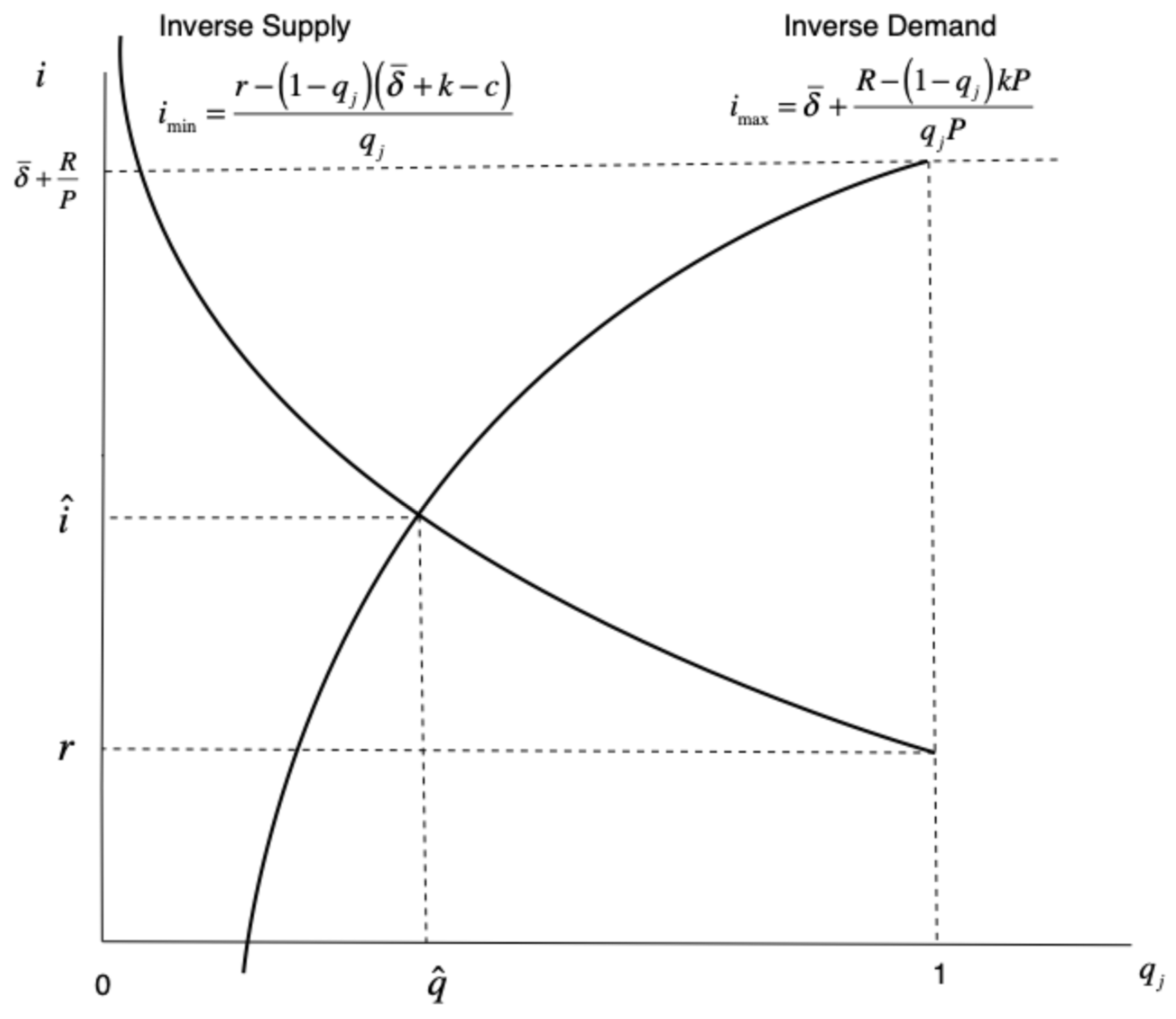
Assuming there are many price-taking lenders, we equate (6) to (9) and solve for the market equilibrium no-default probability, $\widehat{q}$, for the marginal borrower obtaining a mortgage

$$\widehat{q}={\displaystyle \frac{\left(r-\overline{\delta }+c\right)P-R}{Pc}}.$$

(10)

Substituting (10) into (6) or (9), we find the market equilibrium mortgage rate:

$$\widehat{i}=\overline{\delta }+k+{\displaystyle \frac{c\left(R-kP\right)}{\left(r+c-\overline{\delta }\right)P-R}}.$$

(11)

Figure 1 illustrates the market equilibrium.

Several comparative statics of the baseline model are relevant to our investigation. If the expected rate of home price appreciation declines, the inverse demand function shifts downward while the inverse supply function shifts upward, with the former shift being larger, causing the equilibrium mortgage rate to fall and the no-default probability cutoff to rise. Thus, mortgages become less expensive but more difficult to obtain. Other comparative static results are similarly consistent with what we expect to see in practice. A decrease in the bank’s cost of foreclosure causes the inverse supply function to shift down, lowering the equilibrium mortgage rate and marginal no-default probability. Finally, an increase in the T-bill rate causes the inverse supply function to shift upwards, raising the equilibrium mortgage rate and the no-default cutoff.

Turning our attention to a representative bank in the baseline model, we assume that the bank is willing to hold all deposits, which, along with bank equity, help fund two types of loans: mortgages to households, and loans to the federal government in the form of T-bill purchases, which have a safe rate of return $r>0$. We write the bank balance sheet in the baseline model as consisting of two assets and two liabilities, as shown in

Table 2. Bank Balance Sheet.

Assets	Liabilities
Mortgages and rental properties	Demand deposits (Money needed by households at time 1)
T-bills	Equity (To cover losses from mortgage defaults)

.

Consider bank liabilities in the model at time 0. Low-wealth households with $q_j\ge \widehat{q}$ both desire and qualify for a mortgage, while the other low-wealth households with $q_j<\widehat{q}$ end up renting a dwelling. Therefore, the proportion of low-wealth households that obtain mortgages is $\left[1-F\left(\widehat{q}\right)\right]$ and the proportion that rent is $F\left(\widehat{q}\right)$. Since the total number of low-wealth households is $L$, the total value of demand deposits is

$$M_{u}F\left(\widehat{q}\right)L+M_q^T+\overline{M}H,$$

(12)

where $H$ is the number of high-wealth households, and $M_q^T$ is given by (4). From (2), total bank equity is $E_{B}H$. On the asset side, the total value of mortgages at time 0 is $\left[1-F\left(\widehat{q}\right)\right]PL$, while the value of rental income is $F\left(\widehat{q}\right)LR$. Consequently, the value of T-bills is

$$T=M_{u}F\left(\widehat{q}\right)L+M_q^T+\overline{M}H+E_{B}H-\left[1-F\left(\widehat{q}\right)\right]PL-F\left(\widehat{q}\right)RL.$$

(13)

We now assess the possibility of a financial threat triggered by a decrease in home price that results in negative returns to banks. At time 1, the bank makes a profit on each defaulted mortgage of $\left(\delta +k-c\right)P$, which becomes negative if the bank’s gross benefit from foreclosure, $\delta +k$, falls below its cost, $c$. On the other hand, for a mortgage that is paid off, the bank realizes a profit of $iP$. We can write the expected value of $q_j$ for mortgage-qualifying households as $\overline{q}=E\left(q_j\right)|q_j\ge \widehat{q}={\int }_{\widehat{q}}^{1}q·f\left(q|q\ge \widehat{q}\right)dq$. Then, from the LHS of (5), we can write the bank’s expected rate of return on mortgages $\overline{i}$ as

$$\overline{i}=\overline{q}\widehat{i}+\left(1-\overline{q}\right)\left(\overline{\delta }+k-c\right).$$

(14)

The proportion of all mortgages that do not default is $\overline{q}$, the average no-default probability of successful borrowers, while the proportion that default is $1-\overline{q}$. Given that $\widehat{q}$ is the cutoff no-default probability for obtaining a mortgage, it follows that the proportion of low-wealth households that obtain mortgages and do not default is given by $\left[1-F\left(\widehat{q}\right)\right]\overline{q}$ while the proportion of those households that take out mortgages and default is $\left[1-F\left(\widehat{q}\right)\right]\left[1-\overline{q}\right]$.

From their mortgage investments, lenders realize negative time 1 profits if

$$\left[1-F\left(\widehat{q}\right)\right]PL\left\{\left[1-\overline{q}\right]\left(\delta +k-c\right)+\overline{q}i\right\}<0.$$

(15)

But negative mortgage profit will not cause total bank profits to become negative as long as the bank has sufficient positive cash inflows from other sources to cover deposit liabilities. In our model, the other inflows are from Treasuries and invested rental income. Therefore, the bank only realizes negative profits at time 1 if the sum of the net returns from the purchase of T-bills, the appreciated value rental housing, and mortgage investments is less than total demand deposits, $M^T$:8

$$r\left[T+F\left(\widehat{q}\right)RL\right]+\delta \cdot F\left(\widehat{q}\right)PL+\left[1-F\left(\widehat{q}\right)\right]\left[1-\overline{q}\right](\delta +k-c)PL+\left[1-F\left(\widehat{q}\right)\right]\overline{q}iPL<M^T$$

(16)

where $F\left(\widehat{q}\right)RL$ is the value of rental income received at time 0 and immediately invested in Treasuries, and $\delta ·F\left(\widehat{q}\right)PL$ is the appreciation in rental housing.9 Isolating $\delta$ in (16), we can write the critical range for home price appreciation that yields negative bank profit as

$$\delta <{\displaystyle \frac{M^T-r\left(T+F\left(\widehat{q}\right)RL\right)+\left[\left(c-k\right)\left(1-\overline{q}\right)-\overline{q}i\right]\left(1-F\left(\widehat{q}\right)\right)PL}{\left\{F\left(\widehat{q}\right)+\left[1-F\left(\widehat{q}\right)\right]\left[1-\overline{q}\right]\right\}PL}}.$$

(17)

If $\delta$ falls below the RHS of (17), banks face losses due to a low, and possibly negative, rate of home price appreciation for both repossessed homes after mortgage default and rented-out homes. As indicated in (17), the critical value of $\delta$, and therefore the probability of bank non-viability, increases with the cost of foreclosure, but decreases with the values of Treasuries and the mortgage rate.10

Government-sponsored mortgage securitization is frequently heralded as a proactive strategy for reducing the likelihood of bank insolvency caused by adverse changes in home prices. Through securitization, the risks of mortgage defaults are shifted from banks to shareholders in entities like Fannie Mae and Freddie Mac. These shareholders take on the default risk and receive a guarantee fee in return. In the next section, we delve into the impact of securitization on the likelihood and magnitude of negative returns for bank shareholders and investors in GSE equity.

4. The Extended Model with a GSE

We now augment the baseline model to include a government-sponsored securitizer (GSE) that aims to encourage home loans by relieving banks of some default risk while also providing investors with relatively safe investments, GSE equity and mortgage-backed securities. In pursuit of these ends, alongside its overarching objective of profit maximization, the securitizer chooses two parameter values: the minimum credit standard (i.e., no-default probability) that qualifies a mortgage for securitization, and the level of a guaranteed rate of return provided to banks in exchange for swapping mortgages for a mortgage-backed security (MBS), which carries a liquidity/diversification premium11 in addition to the guaranteed rate.

To balance model simplicity and realism, we assume that only wealthy households purchase GSE equity, which offers a positive expected rate of return.12 Wealthy households prefer holding GSE equity over money because, unlike money, it offers a positive expected rate of return along with the implicit backing of the government, which ensures that any downside risk is borne by taxpayers. As in the baseline model, wealthy households can also invest in bank equity and must satisfy a minimum consumption constraint at time 1. The behavior of low-wealth households remains unchanged from the baseline model.

We now modify Problem 1 by adding GSE equity as an investment alternative for wealthy households. We denote the level of this investment by $E_G$ and assume that investors believe the implicit government backing guarantees a positive rate of return, $r_G>0$.13 We can, therefore, write the expected utility maximization problem for the wealthy household as

$$\begin{array}{l}\mathrm{Problem} \mathrm{IV}: \max E(U)=C_0\cdot E\left(C_1\right)\\ \hspace{1em}\hspace{1em}\hspace{1em}\hspace{1em}\hspace{1em}s.t. C_0=W_H-E_B-E_G\\ \hspace{1em}\hspace{1em}\hspace{1em}\hspace{1em}\hspace{1em}\hspace{1em} E\left(C_1\right)=\left(1+{\overline{r}}_B\right)E_B+(1+r_G)E_G\\ \hspace{1em}\hspace{1em}\hspace{1em}\hspace{1em}\hspace{1em}\hspace{1em} \hspace{0.17em}\left(1+r_G\right)E_G\ge \overline{M}\end{array}$$

$\overline{M}>0$ is the amount of cash (from the sale of the MBS) necessary to support survival consumption at time 1.14 Appendix D solves Problem IV and finds

$$E_G={\displaystyle \frac{\overline{M}}{\left(1+r_G\right)}}$$

(18)

and

$$E_B={\displaystyle \frac{W_H}{2}}-{\displaystyle \frac{\left(2+{\overline{r}}_B+r_G\right)\overline{M}}{2\left(1+{\overline{r}}_B\right)\left(1+r_G\right)}},$$

(19)

under the assumption that an investment in bank equity is perceived to have a greater expected return than the return on GSE equity, i.e., ${\overline{r}}_B>r_G$. Equation (18) reveals an intriguing relationship wherein investment in securitizer equity declines as its rate of return increases. This somewhat puzzling result stems from the role of GSE equity investment in the model as a guarantee, ensuring a minimum consumption level at time 1. Consequently, the higher the rate of return, denoted as $r_G$, the less investment ($E_G$) is required at time 0. Equation (19) shows that the size of the wealthy household’s investment in bank equity increases with the expected rates of return on bank equity and GSE equity. Furthermore, we note that the household invests less in bank equity when GSE equity serves as an available option, as shown by comparing (19) and (2).

We now analyze the securitizer’s behavior as a sequential game played in conjunction with a representative bank. At time 0, the securitizer sets the two contractual terms for swapping a mortgage-backed security (MBS) for a mortgage, while knowing the probability distributions for no-default probabilities and for home-price appreciation but not their realized values. During this initial phase, the securitizer establishes a guaranteed interest rate $r_S>0$ offered on the MBS and a minimum credit standard (i.e., no-default probability) $\tilde{q}>0$ that every mortgage must meet to qualify for securitization.

Subsequently, if the bank opts to hold the MBS rather than the mortgage itself, it receives an exogenous liquidity premium, $\tau >0$. This additional compensation factor is independent of the securitizer’s decisions and reflects the specific liquidity advantage associated with holding an MBS. Once the securitizer has set the MBS contractual terms, the bank begins receiving mortgage loan applications. These applications reveal the applicants’ loan default probabilities, which are also observed by the securitizer.

The bank uses the information on default probabilities and MBS contractual terms to decide which households’ mortgage applications will be rejected and which will be offered mortgages. The bank also decides whether to keep these mortgages in the portfolio or immediately swap them for a mortgage-backed security. At time 1, borrowers who have been granted mortgages either default on their mortgages, and obtain a payoff equal to their money holdings minus the costs of default $M_q-kP$, or pay off their mortgage in full, receiving a payoff of $M_q+\left(\delta -i\right)P$, their money holdings plus the difference between the realized house appreciation rate and the mortgage rate multiplied by the original house price.

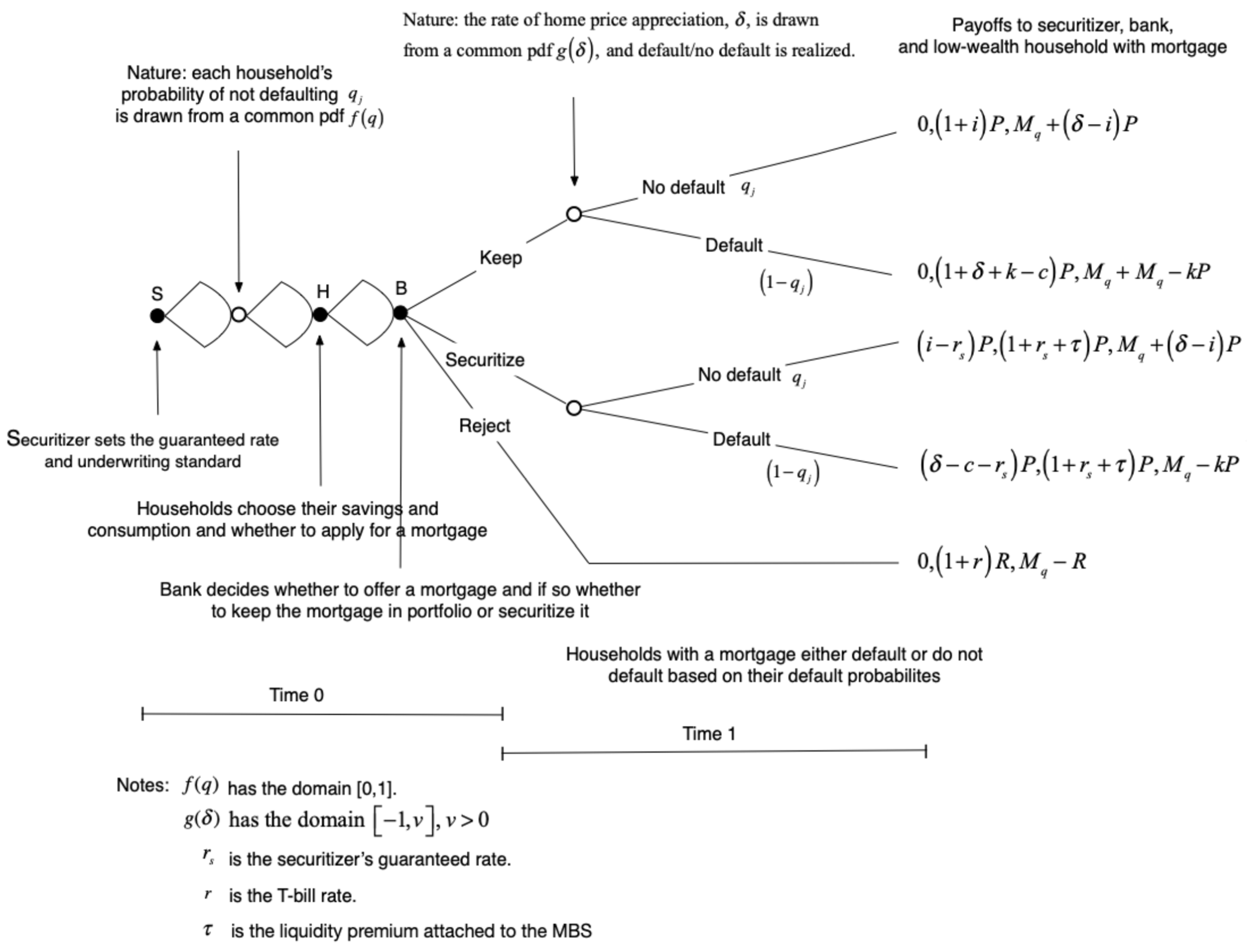
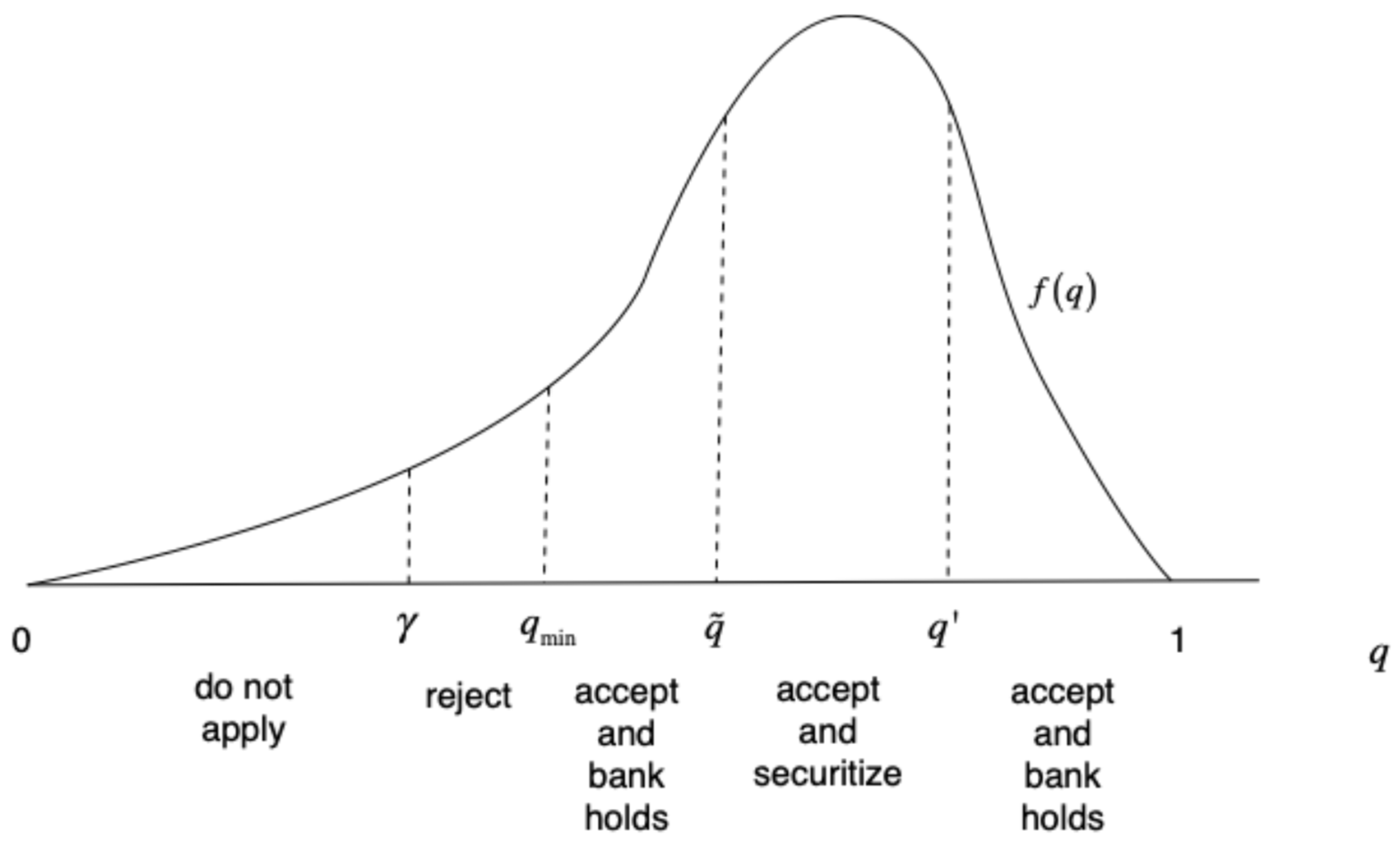
The sequential game is depicted in Figure 2. The securitizer first chooses $r_s$ and $\tilde{q}$. Then, both the bank and securitizer observe the applicants’ default probabilities. For mortgage applications that meet both the bank’s credit cutoff $q_{min}$ and the securitizer’s conforming requirement $\tilde{q}$, the bank decides either to hold the mortgage in its own portfolio or to sell the mortgage to the securitizer. For applications that do not meet the conforming standard, the bank decides whether to offer a mortgage and keep it in portfolio (for $q_j\ge q_{min}$) or reject the application (for $q_j<q_{min}$). Finally, at time 1, borrowers either default or do not default, and all parties (securitizer, bank, and households) receive their payoffs.15

We now shift our attention towards events and actions that could serve as precursors to a financial crisis in the extended model. As in the baseline model, we assume households apply for mortgages if the expected utility from home ownership outweighs that of renting. Consequently, a household applies for a mortgage if inequality (8) is satisfied, which can be rearranged to show the threshold or cutoff no-default probability at which obtaining a mortgage becomes advantageous to the household:

$$q_j\ge {\displaystyle \frac{kP-R}{\left(\overline{\delta }+k-i\right)P}}\equiv \gamma$$

(20)

Households with no-default probabilities less than $\gamma$ do not apply for mortgages. A conforming loan, which qualifies for securitization, must have a no-default probability at least as high as the threshold $\tilde{q}$ set by the securitizer. Thus, the proportion of households that qualify for securitization is $\left[1-F\left(\tilde{q}\right)\right]$ for $\tilde{q}\in \left[0,1\right]$, which is decreasing in $\tilde{q}$.

We now more closely examine the bank’s decision either to accept or reject a mortgage application. As noted earlier, if a particular application is accepted, then the bank either keeps the mortgage in its portfolio or trades it for a mortgage-backed security, if it is conforming. To induce a bank to originate and securitize a mortgage, the return generated from securitization must be at least as great as the alternative return the bank could earn by holding the mortgage in its portfolio. The total return to the bank from securitizing a mortgage is $r_s+\tau$, where $\tau >0$ is the liquidity value to the bank from holding a mortgage-backed security, as opposed to the mortgage itself.

The bank also considers the borrower’s credit quality. To hold a mortgage in its own portfolio, the bank has a minimum requirement for the probability of no default, which is derived from (5). The bank will refuse to hold any mortgage that fails to satisfy (5), implying a probability of default in the interval:

$$q_j<{\displaystyle \frac{r+c-\overline{\delta }-k}{i+c-\overline{\delta }-k}}\equiv q_{\min }.$$

(21)

With the possibility of securitization and assuming the bank’s return to securitization exceeds its alternative return, i.e., $r_s>r$, the bank only rejects a mortgage application if it fails to meet both its own credit standard and that of the securitizer, i.e., $q_j<q_{min}$ and $q_j<\tilde{q}$.

If either of the next two conditions are met, the bank will offer a mortgage and hold it in its own portfolio. The first condition states that the expected return is higher from holding the asset in the portfolio rather than securitizing it: $q_{j}i+\left(1-q_j\right)\left(\overline{\delta }+k-c\right)>r_s+\tau$, which implies that the no-default probability satisfies

$$q_j>{\displaystyle \frac{r_s+\tau +c-\overline{\delta }-k}{i+c-\overline{\delta }-k}}\equiv q^{\prime }.$$

(22)

The next condition stipulates that the no-default probability of the mortgage application satisfies the bank’s minimum requirement but falls below the qualifying standard for securitization:

$$q_{\min }\le q_j<\tilde{q}.$$

(23)

The bank offers and securitizes a mortgage if it qualifies for securitization and the bank finds the swap more profitable than holding the mortgage in its own portfolio:

$$\tilde{q}\le q_j\le q^{\prime },$$

(24)

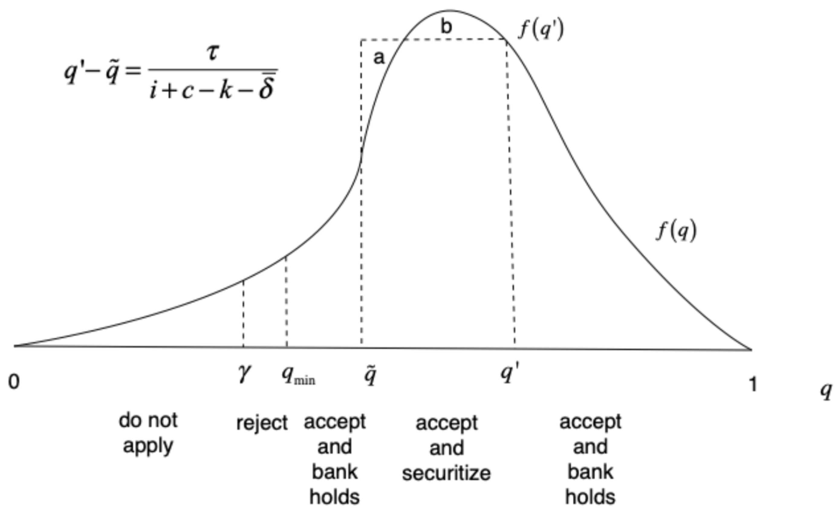
where the securitizer’s choice of $\tilde{q}$ remains to be determined. Figure 3 partitions the probability density function of no-default probabilities into regions indicating mortgage outcomes ranging from no application, to being selected for the bank’s portfolio, to being swapped for a mortgage-backed security.

Inequality (22) reflects the bank’s ability to cherry-pick borrowers with high no-default probabilities by using its first-mover advantage in choosing which mortgages to hold versus securitize, while (23) captures its ability to offer and keep in its portfolio mortgages the securitizer deems lemons, not worthy of securitization. Later in our analysis, we demonstrate that in a particular type of market equilibrium, the securitizer’s cutoff, $\tilde{q}$, collapses and becomes equal to the bank’s rejection cutoff, $q_{min}$, implying that mortgages with the lowest no-default probabilities are securitized.

We now investigate how the securitizer sets the MBS contract terms, which has important effects on the bank’s subsequent mortgage-portfolio decisions and the payoffs to both the bank and securitizer. We assume, while taking as given $i, r, L, P, c,k, f\left(q\right), \mathrm{a}\mathrm{n}\mathrm{d} g\left(\delta \right)$, that the securitizer chooses $\tilde{q}$ and $r_s$ to maximize its expected profit:

$$\underset{\tilde{q},r_s}{\max } {\pi }_s=L{\displaystyle {\displaystyle \underset{\tilde{q}}{\overset{q^{\prime }}{\int }}}f\left(q\right)}\left[q(i-r_s)P+(1-q)(\overline{\delta }+k-c-r_s)P\right]dq.$$

(25)

Assuming positive solutions for $\tilde{q}$ and $r_s$, we compute the following first-order conditions:

$${\displaystyle \frac{\partial {\pi }_s}{\partial \tilde{q}}}=-PLf\left(\tilde{q}\right)\left[\tilde{q}(i+c-k-\overline{\delta })+\overline{\delta }-c+k-r_s\right]=0$$

(26)

and

$${\displaystyle \frac{\partial {\pi }_s}{\partial r_s}}={\displaystyle \frac{PL}{(i+c-k-\overline{\delta })}}f\left(q^{\prime }\right)\left[q^{\prime }(i+c-\overline{\delta })+\overline{\delta }-c+k-r_s\right]-PL{\displaystyle {\displaystyle \underset{\tilde{q}}{\overset{q^{\prime }}{\int }}}f\left(q\right)dq}=0$$

(27)

By prior assumptions, $L, f\left(\tilde{q}\right), P>0$, which implies from (26) that

$$\tilde{q}={\displaystyle \frac{r_s+c-k-\overline{\delta }}{i+c-k-\overline{\delta }}}.$$

(28)

Recalling (22), we see that $q^{\prime }-\tilde{q}={\displaystyle \frac{\tau }{i+c-k-\overline{\delta }}}$, which later we show is positive. Equation (28) shows that the securitizer would earn zero profit by securitizing the marginal qualifying mortgage, a standard profit-maximization result. Together, (26) and (27) imply

$$f\left(q^{\prime }\right)\left(q^{\prime }-\tilde{q}\right)=F\left(q^{\prime }\right)-F\left(\tilde{q}\right)$$

(29)

which geometrically says the area of a rectangle with height $f\left(q^{\prime }\right)$ and width $q^{\prime }-\tilde{q}$ equals the area under the pdf between $\tilde{q}$ and $q^{\prime }$, implying in Figure 4 that areas a and b are equal.

Equation (29) has an appealing economic interpretation. The LHS is the securitizer’s marginal benefit from raising the guaranteed rate $r_s$. A marginal increase in $r_s$ increases the proportion of low-wealth households with securitized mortgages at the upper end of the securitized group at rate $f\left(q^{\prime }\right)$. The marginal increase in $r_s$ also improves the credit quality interval of the securitized group by raising both the upper- and lower-bound probabilities, $q^{\prime }$ and $\tilde{q}$, by the same magnitude. So, the product $f\left(q^{\prime }\right)\left(q^{\prime }-\tilde{q}\right)$ can be interpreted as the change in the securitized proportion times the gain in credit quality, the marginal benefit of raising $r_s$. The RHS of (29) measures the marginal cost of raising $r_s$ as the increased proportion of all low-wealth households that end up with securitized mortgages (costing the securitizer $r_s$). This proportion is increasing at the optimal solution since $f\left(q^{\prime }\right)>f\left(\tilde{q}\right)$ must be true for (29) to hold. In Appendix E, we derive second-order conditions for the securitizer’s problem.

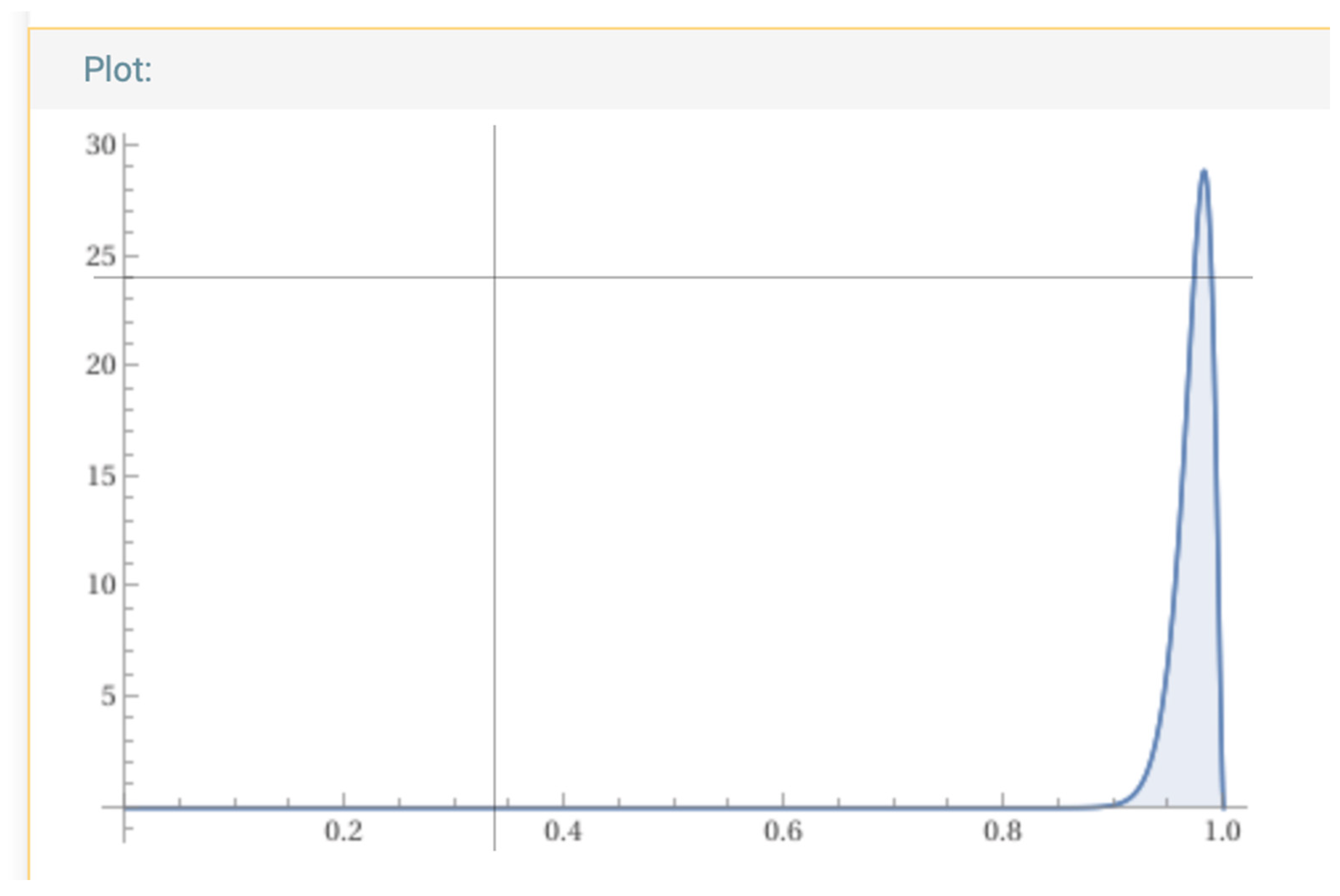
To derive implications regarding the impact of securitization on the likelihood of financial crises, it is essential to obtain an explicit solution for the securitizer’s choice of $r_s$. Furthermore, obtaining this solution requires a specific form for the probability density function of no-default probabilities, $f\left(q\right)$. The Beta distribution,16 often referred to as the ‘probability distribution for probabilities’, provides us with a suitable flexible mathematical form. To estimate the shape parameters, $\alpha$ and $\beta$, of the Beta distribution for $f\left(q\right)$, we use quarterly U.S. data from the period spanning February 2013 to January 2020 on the probability of default on consumer mortgages17. By fitting the Beta distribution to the observed default data, we estimate parameter values $\widehat{\alpha }=98.174$ and $\widehat{\beta }=2.768$. These values reflect the characteristics and behavior of mortgage defaults during the given time frame.18 Plugging these parameter values into the Beta distribution yields $f\left(q\right)=q^{97.174}{(1-q)}^{1.768}/B(98.174,2.768)$, which has the following graph, unsurprisingly left skewed.

For the Beta distribution, shown in Figure 5, the RHS of (29) becomes $F\left(q^{\prime }\right)-F\left(\tilde{q}\right)= {\int }_{\tilde{q}}^{q^{\prime }}{q}^{\alpha -1}{\left(1-q\right)}^{\beta -1}dq/B\left(\alpha ,\beta \right)$, while the LHS becomes $f\left(q\right)\left(q^{\prime }-\tilde{q}\right)=q^{\alpha -1}{\left(1-q\right)}^{\beta -1}\left(q^{\prime }-\tilde{q}\right)/B\left(\alpha ,\beta \right)$.

In Appendix F, we demonstrate that the securitizer’s profit-maximizing MBS rate varies directly with the mortgage rate, a result that is well supported by empirical data and aligns with economic intuition. In our model, this relationship plays a crucial role when securitization lowers both the equilibrium mortgage rate and MBS rate, thereby shrinking bank profit margins on both securitized and retained mortgages. When borrowers enjoy lower mortgage rates from banks, the securitizer seizes the opportunity to offer banks a reduced MBS rate. Doing so improves the securitizer’s profit margin while maintaining bank incentives to securitize those borrowers with no default rates in the gap between $\tilde{q}$ and $q^{\prime }$. Therefore, when securitization successfully lowers the equilibrium mortgage rate, it leads to enhanced access to securitization. Equation (22) shows that the bank holds mortgages with no-default probabilities above $q^{\prime }$, which is decreasing in the mortgage rate for a fixed MBS rate:

$${\displaystyle \frac{\partial q^{\prime }}{\partial i}}{|}_{r_s}={\displaystyle \frac{-\left(r_s+\tau +c-k-\overline{\delta }\right)}{{\left(i+c-k-\overline{\delta }\right)}^2}}<0$$

(30)

From (22) and (28), we know that the gap $q^{\prime }-\tilde{q}$ is decreasing in $i$ after adjustments in $r_s$ are taken into account. Any change in $r_s$ leads to a direct change in $q^{\prime }$ and $\tilde{q}$ by the same magnitude.

Solving (6) for $q_j$ yields the minimum no-default probability that causes the bank to be willing to hold rather than reject a mortgage: $q_{min}=(r+c-k-\overline{\delta })/(i+c-k-\overline{\delta })$. For the bank to favor securitization over investing in T-bills, it must be the case that the return from securitization is greater than or equal to the return on T-bills: $r_s+\tau \ge r$. Substituting (28), which shows how the securitizer’s MBS rate varies with the mortgage rate, into this inequality, we find

$$\tilde{q}\ge {\displaystyle \frac{r+c-k-\overline{\delta }-\tau }{i+c-k-\overline{\delta }}}\equiv {\tilde{q}}_{\min },$$

(31)

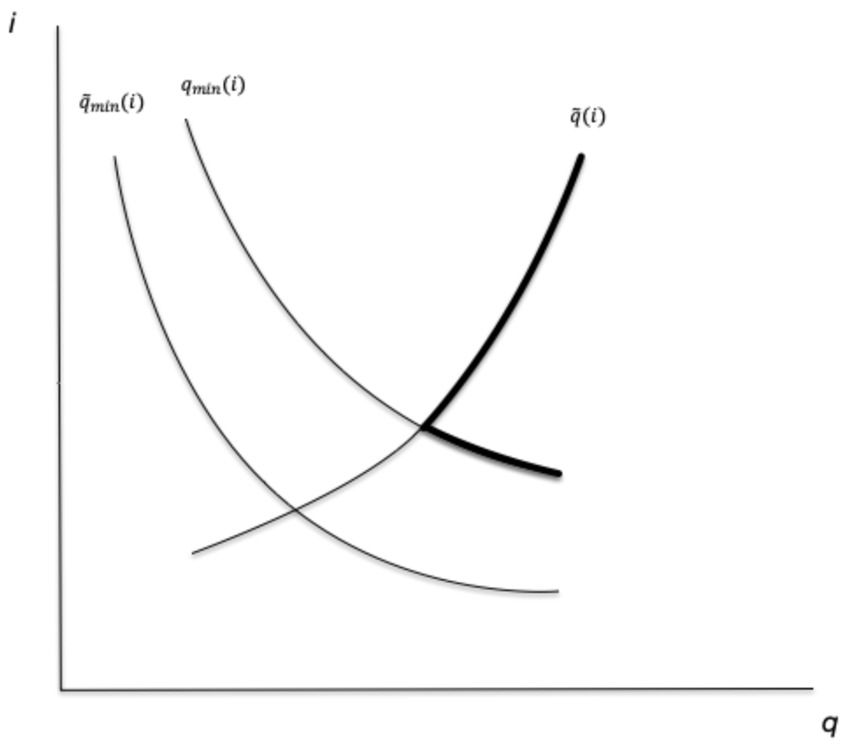
which is the minimum no-default probability for mortgages that banks will accept when they intend to securitize the mortgage. The difference between these two probabilities is $q_{min}-{\tilde{q}}_{min}=\tau /(i+c-k-\overline{\delta })$, which is increasing in $\tau , k, \mathrm{a}\mathrm{n}\mathrm{d} \overline{\delta }$, but decreasing in i and c. The GSE’s willingness to securitize a mortgage depends on the borrower’s no-default probability and the mortgage rate, as shown in Appendix F, which also demonstrates that $\tilde{q}$ increases with i.

For a mortgage to be securitized, both the bank and GSE must be willing to exchange the mortgage (with its risk of default) for the GSE’s guaranteed payment of rate $r_s$ to the bank. At any mortgage rate i, the willingness of both parties to securitize the mortgage is given by the right envelope of the ${\tilde{q}}_{min}\left(i\right)$ and $\tilde{q}\left(i\right)$ functions, shown in bold as the “short side” of the market in Figure 6.

In Figure 6, the bold segments of $\tilde{q}\left(i\right)$ and ${\tilde{q}}_{min}\left(i\right)$ thus show the lowest probability of no default on a securitized mortgage as a function of the mortgage rate. All mortgages plotting to the right of the bold segments are acceptable for securitization.

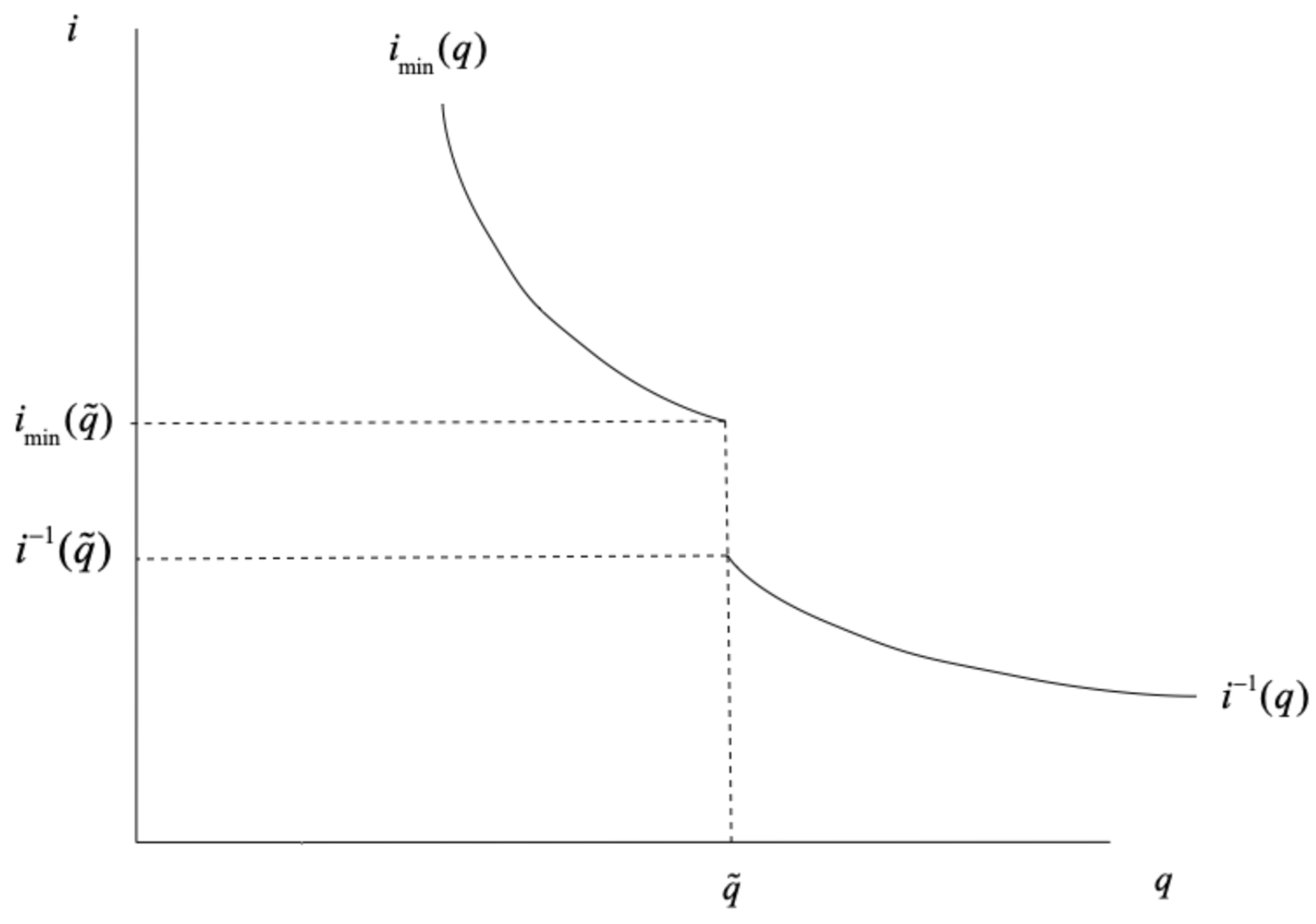
We derive the market inverse supply function as the set of lowest mortgage rates for which a mortgage is offered and held either by the bank or securitizer. For any $q\ge \tilde{q}$, the lowest rate is given by the ${\tilde{q}}_{min}\left(i\right)$ function. In that interval of no-default probabilities, the securitizer is willing and able to hold mortgages at a lower mortgage rate than are banks. In addition, banks are willing to securitize these mortgages at the MBS rate rather than reject them. On the other hand, for $q<\tilde{q}$, the lowest mortgage rate is given implicitly by $q_{min}\left(i\right)$. In the interval $q<\tilde{q}$, the securitizer and bank do not find a mutually agreeable $\left(r_s,\tilde{q}\right)$ combination for securitizing the marginal mortgage. Essentially, the securitizer recoils at the idea of holding mortgages with no-default probabilities below $\tilde{q}$.

Recall that $i_{min}=\overline{\delta }-c+(r+c-k-\overline{\delta })/q_j$ and solve (31) for i to obtain

$$i^{-1}\left(\tilde{q}\right)={\displaystyle \frac{r+\left(1-\tilde{q}\right)\left(c-k-\overline{\delta }-\tau \right)}{\tilde{q}}}.$$

(32)

Thus, the inverse supply function $i_{supply}$ is $i_{min}$ for $q<\tilde{q}$ and $i^{-1}\left(\tilde{q}\right)$ for $q\ge \tilde{q}$, as shown in Figure 7. The discontinuity at $\tilde{q}$ shows that securitization lowers the marginal cost of supplying mortgages to borrowers with good credit risk in the interval $q\ge \tilde{q}$ but has no effect on the supply of mortgages to borrowers with poor credit risk $q<\tilde{q}$. The supply function has a discontinuity at $\tilde{q}$, where it jumps downwards by $i_{min}\left(\tilde{q}\right)-i^{-1}\left(\tilde{q}\right)=\tau /\tilde{q}$. To summarize, the market inverse supply in the extended model is $i_{min}=\overline{\delta }-c+(r+c-k-\overline{\delta })/q_j$ for $q<{\tilde{q}}^{*}$ and $i^{-1}\left({\tilde{q}}_{min}\right)$ for $q\ge {\tilde{q}}^{*}$, as shown in Figure 7.

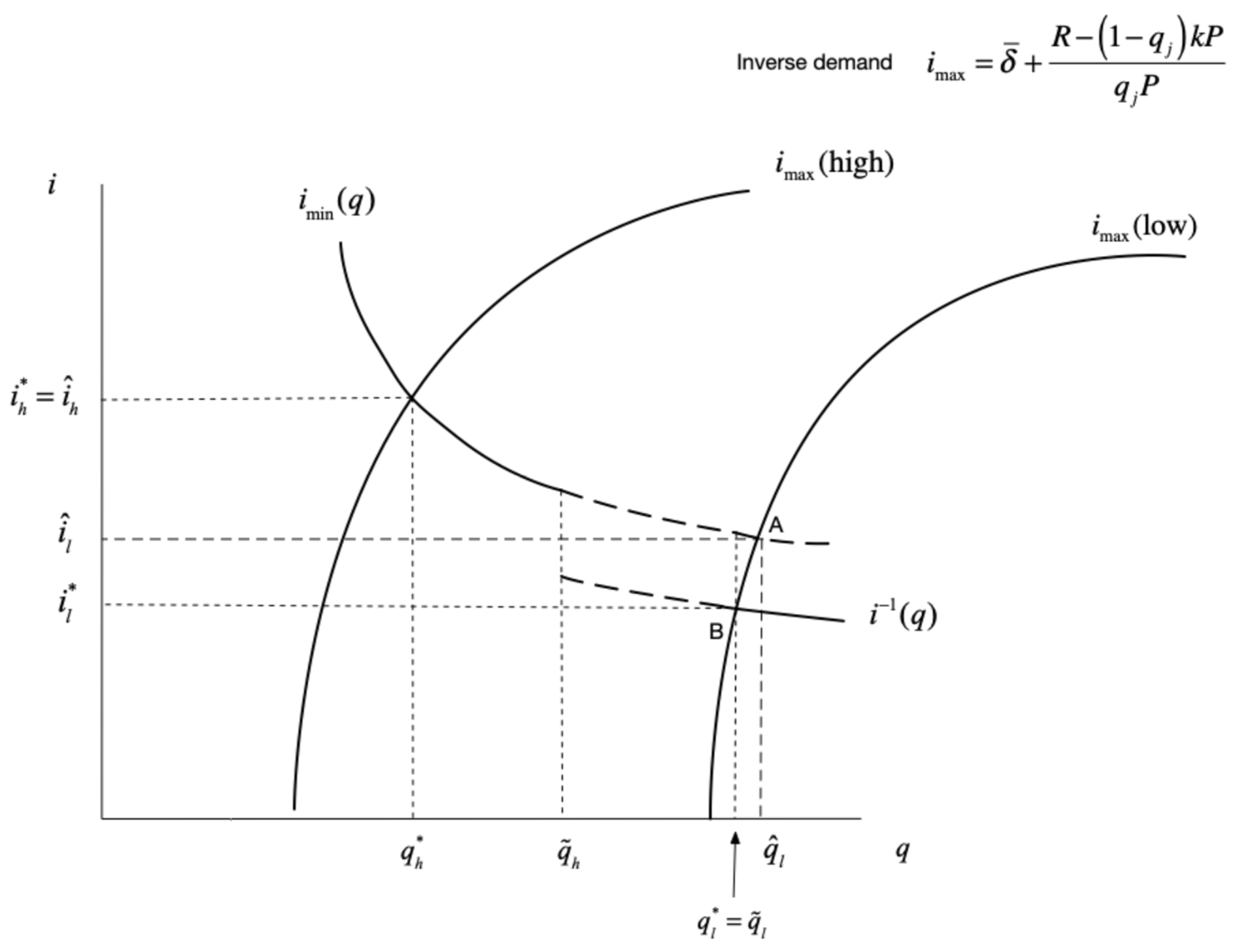
The inverse demand for mortgages remains unchanged between the extended and baseline models. In Figure 8, we graph both the demand and supply functions for the extended model and show two possible equilibria, corresponding to ‘high’ versus ‘low’ demand for mortgages. In situations where mortgage demand is sufficiently high, the market equilibrium is characterized by the bank holding the marginal mortgage. Securitization, in this context, does not affect the equilibrium, yielding the same mortgage rate and marginal no-default probability as in the baseline model. However, when mortgage demand is low enough, the securitizer holds the marginal mortgage in equilibrium and, with its liquidity premium, is able to depress the equilibrium mortgage rate and marginal no-default probability.19 An interesting empirical question, not addressed herein, pertains to the likelihood of either of these two equilibria, especially considering that their probability relies on the value of $\tilde{q}$, determining the position of the discrete jump, which in turn depends on the values of i and $r_s$ according to (28).

In the scenario of high mortgage demand, the equilibrium is characterized by $i_{max}=i_{min}$, where the relevant portion of the demand function is the same as in the baseline model, and generates the same equilibrium marginal no-default probability and mortgage rate, as shown in (10) and (11). This result is attributed to the fact that the securitizer is only willing to securitize mortgages with no-default rates at or above $\tilde{q}$, which exceeds the market equilibrium cutoff with high demand. With high mortgage demand, households exhibit a willingness to pay higher mortgage rates, prompting banks to retain those with low no-default probabilities in their portfolios. It is these marginal mortgages that dictate the equilibrium mortgage interest rate, $i_{high}^{*}={\widehat{i}}_{high}$.

The low mortgage demand equilibrium in the extended model arises from equating the inverse demand $i_{max}\left(q\right)$ and supply $i^{-1}\left(q\right)$ at $\tilde{q}$, which implies

$$q_j={\displaystyle \frac{\left(r+c-\overline{\delta }-\tau -\frac{R}{P}\right)}{c}}={\displaystyle \frac{\left(r_s+c-k-\overline{\delta }\right)}{\left(i+c-k-\overline{\delta }\right)}}=\tilde{q}$$

(33)

Substituting (33) back into $i^{-1}\left(q\right)=\overline{\delta }+k-c+\left(r+c-k-\overline{\delta }-\tau \right)/q_j$, we find the low-demand equilibrium mortgage rate with the GSE:

$$i_{low}^{*}=\overline{\delta }+k-c+{\displaystyle \frac{\left(r+c-k-\overline{\delta }-\tau \right)cP}{\left(r+c-\overline{\delta }-\tau \right)P-R}}$$

(34)

Comparing (34) to the equilibrium mortgage rate given by (11) for the baseline model, we find that the two equations differ only in that the liquidity premium (with a negative sign) appears in the low-demand equation. This analysis shows that for given values of $r, k, c, P, \tau \mathrm{a}\mathrm{n}\mathrm{d} \overline{\delta }$, securitization lowers the equilibrium mortgage rate if demand is “low” (when the securitizer holds the marginal mortgage) but has no effect if demand is “high.”

Another interesting implication of our model pertains to a policy aimed at reducing mortgage rates and expanding accessibility to home ownership. As depicted in Figure 8, an effective approach would involve a government subsidy directed toward banks (achieved by reducing the bank’s foreclosure cost of foreclosure c). By doing so, the northwestern and southeastern20 sections of the inverse supply function would shift downwards, achieving the desired result regardless of whether demand is high or low. Conversely, providing a subsidy to the securitizer that increases the liquidity premium only shifts the southeastern section of the supply function downward, and therefore is only effective if demand is low.

Shifting our focus to empirical matters, we now take parameter values based on U.S. economic data21 and insert them into the first-order conditions for high and low demand, yielding equations with $r_s$ as the only unknown. We develop simulations that offer broad insights into causal relationships, aiming to illuminate overarching patterns rather than furnish precise quantitative predictions applicable to the real world.

Since there is no straightforward closed-form solution for $r_s$, we solve for it iteratively and find for high demand $r_s^h=0.04023$ and $i_{high}^{*}=0.04396=\widehat{i}$.22 Next, we insert the same estimated parameter values into the low-demand equilibrium and solve iteratively for $r_s^l\approx 0.00743$, showing that the securitizer’s guaranteed rate is lower in the low-demand case as compared to the high-demand case.23 Also, the equilibrium mortgage rate $i_{low}^{*}=0.02258$ is below the rate $\widehat{i}$ determined in the baseline model. Furthermore, the equilibrium marginal no-default probability is ${\tilde{q}}_l=0.82088$, which is less than the corresponding value of ${\tilde{q}}_h=0.83049$ in the high-demand case. Thus, in the low-demand scenario, the presence of the securitizer lowers the equilibrium mortgage rate and makes mortgages accessible to households with lower credit worthiness. Graphically, this is shown by a comparison of points A and B in Figure 8.

At this juncture, the model’s results align with the prevailing consensus that government-sponsored mortgage securitization can increase the affordability and accessibility of mortgages. Nevertheless, our primary objective remains focused on examining the risk of financial crisis stemming from the impact of house price appreciation on the profits of both the securitizer and the bank. The securitizer’s profit at time 1, after the realization of $\delta$, is given by

$${\pi }_s=\left[F\left(q^{\prime }\right)-F\left(\tilde{q}\right)\right]PL\left[{\overline{q}}^{‴}i+\left(1-{\overline{q}}^{‴}\right)\left(\delta +k-c\right)-r_s\right],$$

(35)

where ${\overline{q}}^{‴}$ is the average no-default probability for the mortgages that are securitized. If

$$\delta <c-k+{\displaystyle \frac{r_s-{\overline{q}}^{‴}i}{\left(1-{\overline{q}}^{‴}\right)}},$$

(36)

then the securitizer’s profits are negative. Next, we write this inequality using the Beta distribution and the model parameter values specified in the Supplementary Materials spreadsheet. For the high-demand case, we compute ${\overline{q}}_h^{‴}=0.97744$.24 Then, we substitute $r_s^h=0.04023, i_h=0.04396, c=0.26, k=0.17, \mathrm{a}\mathrm{n}\mathrm{d} {\overline{q}}_h^{‴}=0.97744$ into (36), to find ${\delta }_h^s=-0.03142$, which means that in the high-demand case, a 3.142 percent drop in the price of housing is required to cause the securitizer’s profits to become negative. Next, we compute ${\overline{q}}_l^{‴}=0.84230$ for the low-demand case.25 We substitute $r_s^l=0.00743, i_l=0.02258, c=0.26, k=0.17, \mathrm{and} {\overline{q}}_l^{‴}=0.84230.$ into (36) to find ${\delta }_l^s=0.0165$, showing that when demand is low, the securitizer’s profits are negative for any rate of house price appreciation below 1.65 percent. Putting these results together, we can see that the securitizer’s profits are subject to greater downside risk when mortgage demand is low, when the securitizer’s presence brings down the equilibrium mortgage rate, as opposed to when demand is high.

We now focus on the bank’s profitability. The bank earns profit from three segments of the mortgage market. By holding the mortgages of households with low, but profitable, no-default probabilities in the interval $\left[q_{min}^n,{\tilde{q}}_n\right], n=l,k$, the bank earns in the high-demand state

$${\pi }_1^h=\left[F\left({\tilde{q}}_h\right)-F\left(q_{\min }^h\right)\right]PL\left[i_h{\overline{q}}_h^{\prime }+\left(1-{\overline{q}}_h^{\prime }\right)\left(\delta +k-c\right)\right]$$

(37)

where ${\overline{q}}_h^{\prime }$ is the average no-default probability for the profitable but non-qualifying borrowers in the high-demand case. In the low-demand case, the bank does not hold any mortgages with default probabilities below $q_l^{\prime }$, the cherry-picking rate, so that ${\pi }_1^l=0$.

From securitized mortgages, the bank earns in each state

$${\pi }_2^n=\left[F\left(q_n^{\prime }\right)-F\left({\tilde{q}}_n\right)\right]PL\left[r_s^n+\tau \right]$$

(38)

which is always positive. Finally, the bank has profits from qualifying mortgages that are cherry-picked and kept in the bank’s portfolio:

$${\pi }_3^n=\left[1-F\left(q_n^{\prime }\right)\right]PL\left[i_n{\overline{q}}_n^{″}+\left(1-{\overline{q}}_n^{″}\right)\left(\delta +k-c\right)\right],$$

(39)

where ${\overline{q}}_n^{″}$ is the average no-default probability for cherry-picked mortgages kept by the bank. In each state, bank profits become negative in period 2, compelling the bank to draw on its capital buffer, if

$$r\left[T+F\left(q_{\min }^n\right)RL\right]+\left({\pi }_1^n+{\pi }_2^n+{\pi }_3^n\right)<M^T.$$

(40)

In the baseline model, negative bank profits arise if (17) holds. Solutions for $\overline{q}, \widehat{q}, \widehat{i}, F\left(\widehat{q}\right)$ are shown in Supplementary Materials,26 and given these values and the levels of the model’s exogenous variables, we compute the critical house appreciation rate in the baseline case as $\widehat{\delta }=-0.73$. Any change in house price that is more negative than −73 percent causes bank profits to become negative.

For the extended model (with the GSE), we substitute (37), (38), and (39) into (40) and isolate $\delta$ to find that negative bank profit arises in the case of high demand if

$${\delta }_h<c-k+{\displaystyle \frac{M^T-r\left[T+F\left(q_{\min }^h\right)RL\right]-{\pi }_2^h-PL\left\{\left[F\left({\tilde{q}}_h\right)-F\left(q_{\min }^h\right)\right]i_h{\overline{q}}_h^{\prime }-\left[1-F\left(q_h^{\prime }\right)\right]i_h{\overline{q}}_h^{″}\right\}}{\left[F\left({\tilde{q}}_h\right)-F\left(q_{\min }^h\right)\right]PL\left(1-{\overline{q}}_h^{\prime }\right)+\left[1-F\left(q_h^{\prime }\right)\right]PL\left(1-{\overline{q}}_h^{″}\right)}}.$$

(41)

In the low-demand state, the critical house appreciation rate is

$${\delta }_l<c-k+{\displaystyle \frac{M^T-r\left[T+F\left({\tilde{q}}_l\right)RL\right]-{\pi }_2^l-PL\left[1-F\left(q_l^{\prime }\right)\right]i_l{\overline{q}}_l^{″}}{\left[1-F\left(q_l^{\prime }\right)\right]PL\left(1-{\overline{q}}_l^{″}\right)}}.$$

(42)

A key question is whether the RHS of (41) and/or (42) is larger or smaller than the RHS of (17). This comparison will indicate whether a banking crisis is more or less likely with GSE securitization of mortgages. We address this question by running a simulation of the model and finding that the critical rate of home price appreciation that causes negative bank profits with securitization is −58.9 percent with high demand and +2.89 percent with low demand.27

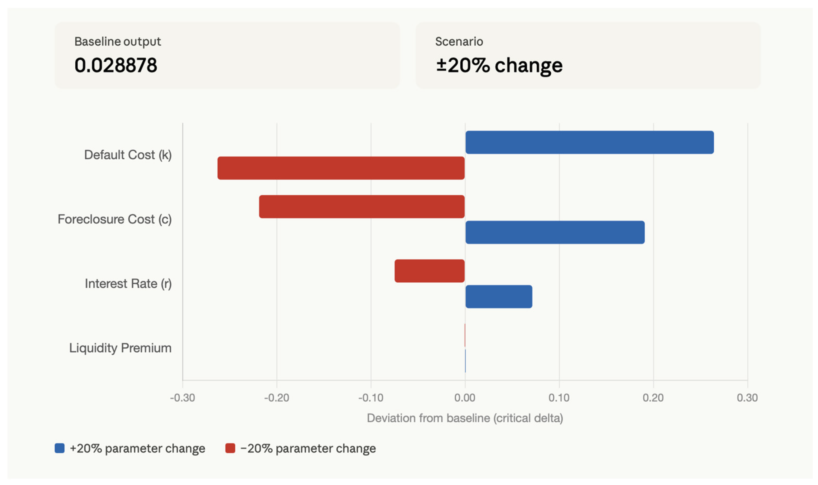
We assess the sensitivity of the model’s results by constructing a tornado chart that shows how the low-demand critical home appreciation rate, which causes bank profits to turn negative, responds to changes in the model’s baseline assumptions.

Figure 9 shows that $\pm 20\%$ changes in the default cost generate the largest variation in the critical home appreciation rate. A 20% increase in k raises the critical rate sharply to 0.29, while a 20% decrease pushes it negative to −0.23. Foreclosure cost c has the second-largest effect, causing the rate to swing between −0.19 and 0.22. These findings reinforce the importance of accurately estimating default and foreclosure costs in any practical application of the model and suggest that this highly abstract framework should be reformulated to better inform economic policy. The T-bill rate has a meaningful but considerably smaller effect than the two cost parameters. A 20% increase in r moves the critical rate to −0.046, and a 20% decrease raises it to 0.1. The liquidity premium has virtually no impact on the critical delta. The model is essentially insensitive to realistic variation in the liquidity premium.

In our modeling exercise, securitization increases the likelihood of financial crisis in the form of bank runs in response to negative bank profits whether demand is high or low, but the threat is greater when demand is low. Securitization poses a risk for banks, even in times of robust mortgage demand, as it grants securitizers the ability to wield first-mover market influence when establishing the guaranteed MBS rate and qualifying standard. These qualitative results are robust to changes in the values of parameters and exogenous variables in the model, even when the quantitative results are significantly affected.28 In the specific example simulated, the securitizer is exposed to potential losses if home price appreciation is more negative than −3.142 percent in the high-demand state and less than 1.65 percent in the low-demand state.29

5. Conclusions

In our model, a systemic financial threat emerges when the change in home prices results in banking assets generating returns that are insufficient to cover deposit liabilities. Our analysis demonstrates a potential impact of government-sponsored securitization in amplifying these threats. It is important to note that the subsequent progression of such threats into full-blown bank failures and other markers of a financial crisis is contingent upon factors outside this paper’s scope. Because our model is structured in only two periods, it cannot capture refinancing decisions or dynamic default behavior.

Our model is based on three key observations about the U.S. economy. First, the process of mortgage securitization serves to transfer credit risk from banks to government-sponsored enterprises. Second, in this process, a sequential game is played between banks and the securitizer, who enjoys a first-mover advantage in setting the terms of the MBS contract in anticipation of bank responses. Lastly, unstable fluctuations in housing prices have proven to be a major catalyst for financial crises.

We have identified both positive and negative effects stemming from mortgage securitization. On the one hand, securitization helps to diversify default risk and, in certain cases, leads to lower mortgage rates and increased loan accessibility for borrowers. On the other hand, these benefits come with important costs: risk is shifted to government-sponsored securitizers and, subsequently, to the public, and banks may be exposed to a greater likelihood of failing to meet their deposit liabilities. A comprehensive welfare analysis lies beyond the scope of this paper, but it remains a promising avenue for future research, particularly for assessing whether the lower mortgage rates associated with securitization adequately compensate for the increased financial risk borne by banks and the public.

Contrary to the belief that securitization safeguards banks, our analysis shows that the opposite is possible: in the context of our model, securitization can expose banks to greater downside risk. Specifically, in the low-demand state, when securitization lowers the mortgage rate, the likelihood of a bank run becomes greater than in the baseline model devoid of securitization. This effect arises because securitization lowers the equilibrium mortgage rate while leaving the average no-default probability of the mortgages held by the bank virtually unchanged,30 thereby cutting into bank profit margins. Interestingly, our model also demonstrates that the securitizer is exposed to more risk precisely when its policies prove effective in expanding mortgage accessibility.

We concede that, in practice, the potency of these threats to induce a financial crisis is diminished when mortgage borrowers provide substantial downpayments, when deposits are government insured, and when robust bank capital requirements and liquidity standards are in place. These measures can ensure that banks maintain sufficient buffers to mitigate losses. Also, the outcomes yielded by our model lend support to the idea that macroprudential policies, such as counter-cyclical capital and liquidity requirements, would be stabilizing. Moreover, our findings align with the notion that government policies of quantitative easing and purchases of distressed assets have the potential to suppress the spread of a financial crisis. Importantly, our model highlights alternative policies to reduce the potential adverse impacts on bank profits by reforming the process for determining the MBS contract. The GSE could charge a fee for securitization that varies with a borrower’s credit risk. Alternatively, securitization could be prohibited for medium-risk mortgages in order to limit banks’ ability to cherry-pick loans. A potential market transformation involves promoting competition in the securitization market by fostering many independent MBS suppliers while also curtailing banks’ discretion in selecting the mortgages for securitization.

References

1. Agarwal, S., Chang, Y., & Yavas, A. (2012). Adverse selection in mortgage securitization. Journal of Financial Economics, 105(3), 640–660. [Google Scholar] [CrossRef] [Scilit]
2. Ambrose, B. W., & Warga, A. D. (2004). Measuring potential gains from mortgage pooling in agency securitization programs. Journal of Money, Credit, and Banking, 36(1), 1–22. [Google Scholar]
3. Becker, J. (2026). Adverse selection in the wholesale mortgage market. Available online: https://ssrn.com/abstract=6115187 (accessed on 16 April 2026).
4. Board of Governors of the Federal Reserve. (2026). Depository institutions: Mortgage and consumer loan portfolios by probability of default. Available online: https://www.federalreserve.gov/releases/efa/efa-project-mortgage-and-consumer-loans-by-probability-of-default.htm (accessed on 16 January 2026).
5. Caballero, R. J., Farhi, E., & Gourinchas, P. O. (2017). The safe assets shortage conundrum. Journal of Economic Perspectives, 31(3), 29–46. [Google Scholar] [CrossRef] [Scilit]
6. Daley, B., Green, B., & Vanasco, V. (2020). Securitization, ratings, and credit supply. Journal of Finance, 25(2), 1037–1082. [Google Scholar]
7. Deku, S. Y., & Kara, A. (2017). Effects of securitization on banks and the financial system. In Securitization: Past, present and future. Palgrave macmillan studies in banking and financial institutions (pp. 93–111). Springer International Publishing. [Google Scholar] [CrossRef] [Scilit]
8. Golec, P., & Perotti, E. (2017, March). Safe assets: A review (European Central Bank Working Paper Series No. 2035). Available online: https://www.ecb.europa.eu/pub/pdf/scpwps/ecbwp2035.en.pdf (accessed on 2 April 2026).
9. Gorton, G. B. (2016, April). The history and economics of safe assets (National Bureau of Economic Research, Working Paper 22210). Available online: https://www.nber.org/system/files/working_papers/w22210/w22210.pdf (accessed on 2 April 2026).
10. Gourinchas, P.-O., & Jeanne, O. (2012, December). Global safe assets. Available online: https://papers.ssrn.com/sol3/papers.cfm?abstract_id=2247974 (accessed on 4 June 2026).
11. He, Z., Krishnamurthy, A., & Milbradt, K. (2016). What makes us government bonds safe assets? American Economic Review, 106(5), 519–523. [Google Scholar] [CrossRef] [Scilit]
12. Heuson, A., Passmore, W., & Sparks, R. (2001). Credit scoring and mortgage securitization: Implications for mortgage rates and credit availability. Journal of Real Estate Finance and Economics, 23(3), 337–363. [Google Scholar] [CrossRef] [Scilit]
13. Kacperczyk, M., Perignon, C., & Vuillemey, G. (2017). The private production of safe assets. IDEAS. [Google Scholar]
14. Kara, A., Ozkan, A., & Altunbas, Y. (2016). Securitization and banking risk: What do we know so far? Review of Behavioral Finance, 8(1), 2–16. [Google Scholar] [CrossRef] [Scilit]
15. Ospina, J., & Uhlig, H. (2018). Mortgage-backed securities and the financial crisis of 2008: A postmortem (NBER Working Paper 24509). IDEAS. [Google Scholar]
16. Purnanandam, A. (2011). Originate-to-distribute model and the subprime mortgage crisis. The Review of Financial Studies, 24(6), 1881–1915. [Google Scholar]
Figure 1. Mortgage Market Equilibrium in the Baseline Model.
Ijfs 14 00167 g001
Figure 2. Sequential game between the securitizer, bank, and low-wealth households.
Ijfs 14 00167 g002
Figure 3. Partitioning the distribution of potential borrowers.
Ijfs 14 00167 g003
Figure 4. The bank and securitizer’s cutoffs, where the difference between the two cutoffs is constant.
Ijfs 14 00167 g004
Figure 5. Beta distribution.
Ijfs 14 00167 g005
Figure 6. Bank and GSE’s willingness to exchange a mortgage for the MBS.
Ijfs 14 00167 g006
Figure 7. Market supply in the extended model.
Ijfs 14 00167 g007
Figure 8. Market equilibrium with high versus low mortgage demand.
Ijfs 14 00167 g008
Figure 9. Tornado chart for sensitivity analysis.
Ijfs 14 00167 g009