Factor Sufficiency in Asset Pricing: An Application for the Brazilian Market

Abstract

The multifactor asset pricing model derived from the Fama–French approach is extensively used in asset risk premium estimation procedures. Even including a considerable number of factors, it is still possible that omitted factors affect the estimation of this model. In this work, we compare estimators robust to the presence of omitted factors in estimating the risk premium in the Brazilian market. Initially, we analyze the panel of asset returns using the mean group and common correlated effect estimators to detect the presence of omitted factors. We then compare the results with those obtained by a estimator robust to omitted variables, which uses a principal components approach to correct the estimation in the case of the omission of latent factors. We conclude that there is evidence of omitted factors, and the best predictor for the expect returns is the common correlated effects estimator.

1. Introduction

Fama and French (1993) introduced the three-factor asset pricing model (Fama and French (1992)), which expanded the traditional capital asset pricing model (CAPM) by identifying three systematic risk factors in stock returns. They constructed these risk factors based on the constructions of portfolios by sorting on stock characteristics. However, subsequent studies, e.g., Titman et al. (2004) and Novy-Marx (2013), suggest that the three-factor model might not be sufficiently comprehensive. In response, Fama and French (1995) extended the model to incorporate profitability and investment factors, resulting in the five-factor model. They found that the five-factor model explains 71%–94% of the cross-sectional variance in expected returns concerning size, book-to-market, profitability, and investment.

Further examination of the Five-Factor Model by Fama and French (2015) across four regions—North America, Europe, Japan, and Asia Pacific—reveals that, while the global model may not provide entirely satisfactory results, regional models, constructed with local data from each area, do a better job in terms of explaining return variance.

The expanding array of potential risk factors in asset pricing has led to the colloquial term “Factor Zoo”. One of the earliest mentions of the Factor Zoo comes from Cochrane (2011), while Harvey et al. (2015), McLean and Pontiff (2016), and more recently, Hou et al. (2017), discuss how the proliferation of new risk factors can influence the risk pricing procedures.

But even with this growing number of new factors, the Fama–French model with 3, 4, and 5 factors continues to be an essential benchmark in risk pricing applications. This is due to the widespread availability of these factors and the interpretability of the associated risk premiums for each factor in the model. However, the existence of many other risk factors highlights the challenges faced when estimating models based on three, four, or five factors derived from the Fama–French framework. These estimations may face difficulties due to the omission of significant risk factors, rendering the risk premium estimates for the incorporated factors unreliable due to the bias generated by variable omission in the econometric estimation.

Recognizing the significance of omitted factors in risk premium estimation, Giglio and Xiu (2021) (referred to as GX) introduced a three-step method for estimating the risk premium of an observable factor. This method remains valid even in the presence of omitted risk factors in the model. It also accounts for possible measurement errors in the observable factors and identifies factors that may be spurious or “useless” in influencing the estimation.

In our study, we analyzed the performance of the Fama–French five-factor pricing model in pricing risk in the Brazilian financial market. The Brazilian financial market exhibits distinctive characteristics when compared to other developing economies. One notable aspect is its technological advancement, stemming from periods of hyperinflation witnessed in the 1980s and 1990s. This tumultuous economic backdrop spurred the development of a sophisticated banking and financial infrastructure. Innovative financial products, including indexed accounts and pioneering instruments like future contracts tied to one-day interbank interest rate fluctuations, emerged as a response to daily price variations. Another significant feature is the market’s size and banking concentration. As of 2021, the five largest banks command over 75% of the market share, exemplifying considerable dominance within the sector.

A unique aspect is the consolidation of operations within the Brazilian financial market. Since the early 2000s, various regional stock exchanges—such as São Paulo (BOVESPA), Rio de Janeiro (BVRJ), Minas-Espírito Santo-Brasília (BOVMESB), among others—were integrated. This led to the concentration of share trading in Brazil, culminating in the merger of BM&F (Bolsa de Commodities and Futures) and Bovespa in 2008, creating BM&FBovespa. This merger unified stock, derivatives, and futures operations under one exchange. Subsequently, the 2017 merger between BM&FBovespa and CETIP, responsible for electronic custody systems and financial settlement in public and private securities markets, further centralized operations. As a result, trading shares, derivatives, futures, and custody and financial settlement systems became centralized under a single market operator. B3 (Bolsa Brasil Balcão), the current name of BM&Fbovespa, stands as Latin America’s largest stock exchange, both in total market capitalization and the number of listed companies.

An integral aspect of the Brazilian financial market is its susceptibility to both political dynamics and the broader global financial landscape. For instance, notable outliers emerged in March 2016 following the exposure of recordings implicating President Luiz Inácio Lula da Silva in the Lava-Jato operation. Similarly, the market experienced significant upheaval in May 2017 when revelations from the JBS partners’ plea bargain involving President Michel Temer rattled investor confidence. Moreover, periods of systemic crises, such as the substantial fluctuations in returns witnessed between September and November 2008, were directly linked to the global financial crisis. Similarly, the onset of the COVID-19 pandemic in March 2023 marked another phase of market turbulence, underlining the interconnectedness between global events and the Brazilian financial landscape.

The Brazilian market also stands out for its sophisticated portfolio and risk management practices, boasting a substantial number of portfolio managers. For instance, as of November 2023, there are 36,255 active registered funds, encompassing 1418 fixed-income funds and 3418 actively managed multi-market funds. Many of these multimarket funds operate on quantitative strategies rooted in factor investing, using multifactor pricing models to create trading strategies, with a central role of models based on risk factors built from characteristics using the Fama–French framework.

There is extensive literature discussing the application of the Fama–French pricing structure to the Brazilian market. The performance of models based on the Fama–French risk pricing structure in the Brazilian market is analyzed in Araújo et al. (2021); Carvalhal (2017); Malaga and Securato (2004); Rayes et al. (2012); Securato and Rogers (2009); Varga and Brito (2016); and Alles Rodrigues and Casalin (2022); Caldeira et al. (2013); Faria Maciel et al. (2021); Rostagno et al. (2006); Silva Moreira and Torres Penedo (2018) directly discuss the use of these models in creating investment strategies.

We study two ways of using the five-factor model to price stocks with Brazilian data. The Fama–French factors are widely used in risk pricing in the Brazilian market, even in the presence of models with alternative risk factors, as discussed in Varga and Brito (2016), but as we discussed, the risk premium estimates derived from this specification may be biased by the omission of relevant factors in the model.

First, we focused our study on testing possible factor omission, and thus the existence of bias in the risk premium estimation. For this, we propose a test for factor omission exploring the panel data structure of asset returns. We apply two estimators for panel data to estimate the risk premium of the factors: the Mean Group (MG), proposed by Pesaran and Smith (1995), and the common correlated effects estimator (CCE), introduced by Pesaran (2006). The MG estimator is defined as an average of OLS estimators, while the CCE estimator is an extension of the MG estimator that assumes an unobserved common factor structure for the errors. Thus, we can interpret the MG estimator as an estimator that is not robust to the presence of omitted risk factors using a panel data structure, while the CCE estimator would be robust to this problem.

If there are factors omitted in the Fama–French five-factor model, the CCE estimator for the parameters of observed factor must be robust for the omission of relevant factors, and therefore, their coefficients would be different from the estimated coefficients for the MG estimator, and we can use the parameter difference between the two estimations to implement a test for factor omission exploring the panel data structure of asset returns.

The second way of studying the relevance of the five factors was to test whether they are sufficient to correctly price the assets, that is, whether these factors can estimate an approximately correct price for the set of assets in question. For this, we estimate the risk premium using the Giglio and Xiu (2021) method, denoted by GX, which theoretically also corrects the estimation for the possible omission of variables and the presence of measurement error using an alternative methodology incorporating the specific aspects of the risk pricing structure, and we use this estimate to predict returns. Finally, we compare which model best fits the observed returns, the MG, CCE, or the GX estimators.

We noticed significant differences in the estimated coefficients for the model when using the MG and CCE estimators, which indicated the potential omission of factors in the model. We also assessed the number of factors that the estimator introduced by Giglio and Xiu (2021) using four penalty functions. Although all penalty functions approached zero as the sample size and time period increased, we were unable to identify a suitable penalty function that ensured accurate factor estimation. Nevertheless, the Giglio and Xiu (2021) estimator performed well with three of the penalty functions, particularly in simulations involving one or three factors.

In comparing the residuals generated by the Fama–French model estimated by the MG, CCE, and GX estimators, the CCE estimator, it was expected that the estimator that the GX three-step estimator would yield superior results. However, it did not perform as well as we had expected in terms of fitting the expected returns. We believe that this might be due to the presence of weak latent factors in the cross-section of the returns, violating one of the main assumptions of the Giglio and Xiu (2021) method.

This study contributes to the field of asset pricing by introducing a novel approach for factor omission testing using panel data, comparing the mean group and common correlated effect estimators to identify the potential missing risk factors in the model. Additionally, the study assesses the sufficiency of the Five-Factor Model in accurately pricing assets, providing insights into its ability to estimate expected returns using the MG, CCE, and GX methods. These contributions are particularly relevant in the Brazilian market, where accurate risk premium estimation is vital for investment decisions, and the study’s methodologies offer valuable insights for researchers and practitioners in finance.

This work has the following structure: a brief literature review is presented in Section 2; the methodology is reviewed in Section 3. In Section 4, we will present the data used. Section 5 presents the main results obtained. Final conclusions are presented in Section 6.

2. Literature Review

The field of asset pricing has witnessed significant advancements in recent years, driven by the emergence of various factors and factor models aimed at understanding how specific characteristics influence asset prices. The foundational work in this domain can be traced back to the portfolio selection problem initially introduced by Markowitz (1952). This work laid the groundwork for optimal portfolio selection, emphasizing the mean variance principle and the creation of efficient mean-variance combinations. Building upon this, Sharpe (1964) proposed a market equilibrium theory of asset prices under risk, revealing a linear relationship between expected returns and the standard deviation of returns for efficient asset combinations. Additionally, Sharpe (1964) highlighted the consistent relationship between expected returns and systematic risk, measured by market beta, which quantifies a stock’s volatility relative to the market.

Similar to Sharpe’s work, Lintner (1965) and Black (1972) also studied the relationship between average returns and risk. Like the Sharpe model, the Lintner (1965) and Black (1972) models concluded that expected returns are positive linear functions of market betas. They also found that market betas absorb the effect of leverage on prices and are sufficient to describe the cross-section of expected returns.

Similarly, Lintner (1965) and Black (1972) explored the connection between average returns and risk, confirming that expected returns exhibit a positive linear relationship with market beta. They also noted that market beta encapsulates the effects of leverage on asset prices and effectively describes the cross-section of expected returns. Meanwhile, Fama and Macbeth (1973) investigated the relationship between dividend yields and expected stock returns, discovering that dividend yields explain a substantial portion of variance in long-term returns but less in monthly or quarterly returns. Fama and French (1988) delved into the relationships between expected returns, market beta, size, leverage, book-to-market equity (BE/ME), and earnings/price (E/P), concluding that leverage is well captured by book-to-market equity, and the combination of size and book-to-market equity accounts for the relationship between E/P and expected returns.

Fama and French (1992) expanded on their previous research using the time series regression approach to construct two risk factors related to size and BE/ME for stocks, and two risk factors related to the term structure for bonds. The factors related to size and BE/ME are known as SMB and HML, respectively. To build these factors, they sorted the stocks by size (big and small) and BE/ME (low, medium, and high). This classification by BE/ME is based on dividing the stock population into three groups, with the lower 30% classified as low, the middle 40% as medium, and the upper 30% as high. From this classification, six portfolios are created based on the intersections between the size and BE/ME classifications: Small/Low (S/L), small/medium (S/M), small/high (S/H), big/low (B/L), big/medium (B/M), and big/high (B/H). These six portfolios provide returns on the large- (B) and small- size (S) portfolios.

$$\begin{array}{cc}\hfill R_B& =\frac{1}{3}(R_{B/l}+R_{B/m}+R_{B/h})\hfill \\ \hfill R_S& =\frac{1}{3}(R_{S/l}+R_{S/m}+R_{S/h})\hfill \end{array}$$

From these two portfolio returns shown above, with $R_B$ and $R_S$ representing the returns of big stocks and the returns of small stocks, respectively, the returns $R_{SMB}$ of zero SMB net investment factors (small minus big, i.e., long position in low capitalization stocks and short position in high capitalization stocks), are constructed:

$$\begin{array}{c}\hfill R_{SMB}=R_S-R_B\end{array}$$

Similarly, the returns of the high (H) and low (L) portfolios are:

$$\begin{array}{c}\hfill R_H=\frac{1}{2}(R_{S/h}+R_{B/h})\\ \hfill R_L=\frac{1}{2}(R_{S/l}+R_{B/l})\end{array}$$

From these two portfolios, the zero HML net investment factor is created (high minus low, that is, a long position in high BE/ME and short position in low BE/ME):

$$\begin{array}{c}\hfill R_{HML}=R_H-R_L.\end{array}$$

They also created two portfolios to measure the common risk related to unexpected changes in interest rates for bonds, called TERM and DEF. These five factors were found to effectively explain the common variation in bond and stock returns.

In a subsequent study, Fama and French (1993) sought to identify the economic foundations for their empirical findings and rationalize asset pricing. They hypothesized that common risk factors associated with size and BE/ME influenced returns, which should be explicable by the earning behavior. However, they did not find evidence supporting the idea that returns respond to the BE/ME factor in earnings, leaving questions open regarding the economic variables influencing earnings and returns related to size and BE/ME.

Despite the popularity of the three-factor model, studies such as those by Titman et al. (2004) and Novy-Marx (2013) revealed its inadequacy in explaining the variations in average returns related to factors like profitability and investment. To address these limitations, Fama and French (1995) introduced the five-factor asset pricing model. This extended model incorporates profitability and investment factors, represented by the Robust Minus Weak (RMW) and conservative minus aggressive (CMA) portfolios, which capture the differences in returns between companies with strong and weak profitability and between conservative and aggressive firms, respectively. This model has demonstrated a superior performance in explaining the average returns compared to the previous three-factor model. However, the potential for omitted variable bias and measurement errors poses challenges, leading to inconsistent estimates and less accurate asset pricing predictions.

To confront these issues, researchers have explored new factors for asset pricing, resulting in a proliferation of potential factors, often referred to as the “Factor Zoo”. Cochrane (2011) was among the first to draw attention to this phenomenon, and subsequent studies, including those by Harvey et al. (2015), McLean and Pontiff (2016), and Hou et al. (2017), have further explored the impact of these factors on pricing models.

As examples of new risk factors, Roy and Shijin (2018) added a human capital factor to the Fama–French estimation. Dirkx and Peter (2020) analyzed a specification based on six risk factors for the German market, and Roy (2023) checked whether a six-factor model works to price global returns. A new risk factor based on equity duration was introduced by Mohrschladt and Nolte (2018), and risk factors linked to tail risk are discussed, for example, in Kelly and Jiang (2014) and Fan et al. (2022). Cho and Jang (2023) tested an alternative specification of risk factors based on durable consumption. A new area of research in finance is linked to the construction of climate risks, e.g., Campiglio et al. (2023), Venturini (2022) and Barasal Morales et al. (2023).

Other examples of six-factor models include those of Roy (2021) and Zhou et al. (2022), and the applications of arbitrage-based pricing models with seven or more risk factors are discussed in Bhatti and Mirza (2014); Maharani and Narsa (2023); Malhotra et al. (2023) and Fang and Almeida (2019), for example. All of these references indicate the need to use a greater number of factors than the usual five factors of the Fama–French structure, indicating that models with a reduced number of factors may be incorrectly specified, requiring the type of corrections for omitted factors discussed in our article.

These works underscore the challenge of omitting relevant factors in risk premium estimation. In response, Giglio and Xiu (2021) proposed a three-step methodology that incorporates rotation invariance and principal component analysis (PCA) to provide consistent risk premium estimates for observed factors, even in the presence of omitted factors and model mis-specification. This approach addresses critical issues in risk premium estimation and offers a path towards more robust asset pricing models.

A general discussion on risk pricing models, and particularly regarding econometric methods for estimating these models, can be found, e.g., in Campbell et al. (1997), Cochrane (2005) and Fan and Yao (2015). Our analysis focuses on frequentist estimation methods, but Bayesian methods can also be used in this context, such as Harvey and Zhou (1990); Hwang and Rubesam (2020); de Andrade Alves and Laurini (2023) and Bryzgalova et al. (2023).

3. Risk Premium Estimation Methodology

In this work, we will assume that the heterogeneity in the cross-section of assets can be summarized through a panel structure, with the general specification:

$$\begin{array}{cc}\hfill R_{it}={\beta }_i^{\prime }{d}_t+e_{it},& \hfill i=1,\dots ,N\end{array}$$

(1)

and, specifically, we use the structure:

$$\begin{array}{cc}\hfill {\beta }_i=\left[\begin{array}{c}{\alpha }_i\\ {\beta }_{iM}\\ {\beta }_{iSMB}\\ {\beta }_{iHML}\\ {\beta }_{iIML}\\ {\beta }_{iWML}\end{array}\right],& \hfill d_t=\left[\begin{array}{c}1\\ R_{Mt}-R_{ft}\\ SM{B}_t\\ HM{L}_t\\ IM{L}_t\\ WM{L}_t\end{array}\right]\end{array}$$

(2)

• $R_{Mt}$ is the market return in period t;
• $R_{ft}$ is the risk free in period t;
• $SM{B}_t$ is the factor related to size in period t;
• $HM{L}_t$ is the factor related to BE/ME in period t;
• $IM{L}_t$ is the factor related to liquidity in period t;
• $WM{L}_t$ is the factor related to past returns (momentum) in period t.

This model is based on the Fama–French five-factor model (Fama and French (1995)). What differs from the Fama–French model are the liquidity ($IML$) and past returns ($WML$) factors that replace the profitability ($RMW$) and investment ($CMA$) factors. This substitution of factors was necessary because our objective was to carry out the study with the factors available through the NEFIN—Brazilian Center for Research in Financial Economics of the University of São Paulo, and the main source of risk factors used in the Brazilian financial market.

3.1. Testing the Sufficiency of Factors

Our objective is identify the presence of omitted factors in the model (1), using a simple diagnosis comparing the estimation of a non-robust panel data model to the presence of omitted factors (mean group estimator—MG) with a robust estimator for panel data in the presence of latent factors, given by the common correlated effects ($CCE$) estimator. Note that the use of a panel in risk premium estimation is a common procedure in factor risk premium estimation, and can be thought of as an alternative estimation method in relation to the Fama–Macbeth procedure (Cochrane (2011)), and the use of panel models for estimating multifactor models is discussed in Petersen (2009).

The MG estimator is a simple average of the OLS estimators of each group, while the CCE estimator is an extension of the MG estimator assuming unobserved common correlated factors in the errors. So, the idea behind the CCE estimator is the same as the one we want to test. For this reason, we chose to compare the Mean Group with the CCE. In the next subsections, we will detail these estimators in more detail.

3.1.1. Mean Group Estimator

To obtain the Mean Group estimator for the heterogeneous panel data model (1), we consider the following matrices:

$$\begin{array}{c}\hfill D={\left[\begin{array}{cccc}{d}_1& d_2& \dots & d_T\end{array}\right]}^{\prime }\end{array}$$

(3)

$$\begin{array}{c}\hfill R_{i.}={\left[\begin{array}{cccc}{R}_{i1}& R_{i2}& \dots & R_{iT}\end{array}\right]}^{\prime }\end{array}$$

(4)

with $R_i$ representing the returns of assets i and $d_i$ and the risk factor i.

The first step was to calculate the OLS estimators of each ${\beta }_i$, according to the equation below:

$$\begin{array}{c}\hfill {\widehat{\beta }}_i={\left(D^{\prime }D\right)}^{-1}{D}^{\prime }{R}_{i.}\end{array}$$

(5)

Finally, we obtain the MG estimator according to the equation below:

$$\begin{array}{c}\hfill {\widehat{\beta }}^{MG}=\frac{1}{N}\sum _{i=1}^N{\widehat{\beta }}_i\end{array}$$

(6)

3.1.2. Common Correlated Effects Estimator

Introduced by Pesaran (2006), the common correlated effects assume that the error in the equation of interest in a panel data structure has a factor structure, and that explanatory variables are linear functions of the latent factors appearing in the estimated equation. The control for the latent factors by the CCE estimator is made by treating the cross-sectional averages of the dependent and explanatory variables as fixed effects, and in this way, asymptotically eliminating the unobserved heterogeneity caused by the omission of the factors in the estimated equation. If we consider a linear risk pricing structure, and the omitted risk factors can be written as portfolios of returns, as in the Fama–French framework, we are meeting the assumptions of this estimator, which allows us to consider the use of this estimator as a control for the omission of risk factors in the risk premium estimation.

To calculate the common correlated effects estimator, we consider the heterogeneous panel data model (1) and assume that the error $e_{it}$ has the following common factor structure

$$\begin{array}{c}\hfill e_{it}=\sum _{j=1}^m{\gamma }_{ij}{f}_{jt}+{\epsilon }_{it}={\gamma }_i^{\prime }{\mathbf{f}}_t+{\epsilon }_{it}\end{array}$$

(7)

where ${\mathbf{f}}_t$ $={\left(f_{1t},\dots ,f_{mt}\right)}^{\prime }$ is a vector of unobserved common factors and ${\gamma }_i={\left({\gamma }_{i1},\dots ,{\gamma }_{im}\right)}^{\prime }$ is the factor loading vector. We assume that the number of factors, m, is fixed, and $m<<N$, where N is the number of assets.

So, substituting (7) into (1), our model has the following form:

$$R_{it}={\beta }_i^{\prime }{d}_t+{\gamma }_i^{\prime }{\mathbf{f}}_t+{\epsilon }_{it}$$

(8)

The common correlated effects (CCE) estimator consists of approximating the linear combination of unobserved factors by means of the cross-section of the dependent and explanatory variables, and then calculating the regression for the augmented standard panel with the averages of the cross-section.

To calculate the averages, we consider a non-stochastic vector of weights ${\mathbf{w}}_t$ $={\left(w_{1t},w_{2t},\dots ,w_{Nt}\right)}^{\prime }$, for $t\in \mathcal{T}\subset \mathbb{Z}$, where $\mathcal{T}$ is our time horizon. The vector ${\mathbf{w}}_t$ was chosen to satisfy the two hypotheses below:

$$\begin{array}{cc}\hfill \left|{\mathbf{w}}_t\right|& ={\left({\mathbf{w}}_t^{\prime }{\mathbf{w}}_t\right)}^{\frac{1}{2}}=O\left(N^{-\frac{1}{2}}\right),\hfill \end{array}$$

(9)

$$\begin{array}{cc}\hfill \frac{w_{jt}}{\left|{\mathbf{w}}_t\right|}& =O\left(N^{-\frac{1}{2}}\right)\mathrm{uniformly}\mathrm{in}\mathrm{j}\in \mathbb{N}.\hfill \end{array}$$

(10)

Thus, the averages were calculated as follows

$$\begin{array}{c}\hfill {\overline{R}}_{wt}={\overline{\beta }}_w^{\prime }{d}_t+{\overline{\gamma }}_w{f}_t+{\overline{\epsilon }}_{wt}\end{array}$$

(11)

where

$$\begin{array}{c}\hfill {\overline{R}}_{wt}=\sum _{i=1}^N{w}_i{R}_{it},{\overline{\beta }}_w=\sum _{i=1}^N{w}_i{\beta }_i,\end{array}$$

(12)

$$\begin{array}{c}\hfill {\overline{\gamma }}_w=\sum _{i=1}^N{w}_i{\gamma }_i,{\overline{\epsilon }}_{wt}=\sum _{i=1}^N{w}_i{\epsilon }_{it}\end{array}$$

(13)

And, from the model’s regression (11), we calculated $f_t$ and ${\widehat{{\beta }_i}}^{CCE}$.

The robustness properties of CCE estimators and its extensions when $T\to \infty$ are further analyzed by Chen and Yan (2019); Chudik and Pesaran (2015); De Vos and Westerlund (2019); Kapetanios et al. (2021); Karabiyik et al. (2019); Westerlund (2018); Westerlund and Urbain (2013, 2015). In our work, we will compare the use of the CCE estimator relative to the estimator based on the principal components proposed by Giglio and Xiu (2021). In this aspect, a discussion of the properties of estimators based on cross-sectional averages versus estimators based on principal components can be found in Westerlund and Urbain (2015), which discusses the bias and efficiency properties of these two formulations in diverse settings.

3.1.3. Wald Tests

The idea of comparing the MG and CCE estimators is to identify the possible presence of omitted factors in the estimation, since the CCE estimator assumes a structure of unobserved common factors for the errors. By estimating the MG and the CCE, we obtained their coefficients and the asymptotic covariance matrices of the parameters for the model (1). We chose to perform the Wald test, since it consists of evaluating the restrictions on the statistical parameters based on the weighted distance between the unconstrained estimate and its hypothetical value under the null hypothesis. The general form of the Wald test is

$$Wald={({\beta }^{\mathrm{MG}}-{\beta }^{\mathrm{CCE}})}^{\prime }{\left[\mathrm{Var}\left({\beta }^M\right)\right]}^{-1}({\beta }^{\mathrm{MG}}-{\beta }^{\mathrm{CCE}})$$

The test distribution under the null hypothesis is a chi-square with the number of degrees of freedom given by the number of tested constraints. Note that we can perform this test in three ways, depending on the parameter covariance matrix $\mathrm{Var}\left({\beta }^M\right)$ used in the test. We can test whether the parameters of the estimations using the MG and CCE estimators are equal under the null using the variance matrix of the MG model estimation ($\mathrm{Var}\left({\beta }^M\right)=\mathrm{Var}\left({\beta }^{\mathrm{MG}}\right)$) or the covariance matrix of the CCE estimator in the Wald test ($\mathrm{Var}\left({\beta }^M\right)=\mathrm{Var}\left({\beta }^{\mathrm{CCE}}\right)$). A third way, which is equivalent to a Hausman test (Hausman 1978), is to test the equality of parameters using the difference between the variance matrices estimated for each model as the test variance matrix, considering the uncertainty associated with estimating the parameters in the two models:

$$Hausman={({\beta }^{\mathrm{MG}}-{\beta }^{\mathrm{CCE}})}^{\prime }{\left[\mathrm{Var}\left({\beta }^{\mathrm{MG}}\right)-\mathrm{Var}\left({\beta }^{\mathrm{CCE}}\right)\right]}^{-1}({\beta }^{\mathrm{MG}}-{\beta }^{\mathrm{CCE}})$$

Finally, a fourth way to test parameter equality is to perform a test of the equality of variances between the two estimations, in an analysis of a variance procedure.

3.2. Giglio and Xiu (2021) Method

We describe the fundamental elements of the three-step estimator proposed by Giglio and Xiu (2021) in this section. The general idea is to use a principal component estimation to recover the effects of the systematic factors omitted from the model, and thus carry out a consistent estimation of the risk premium associated with the factors included in the model. To perform the first step, a consistent estimator of the number of factors is needed, and the number of latent factors must be selected using some statistical criteria.

The estimator used by Giglio and Xiu (2021) share the same components of the factor estimators proposed by Bai and Ng (2002) and Bai (2003). Bai (2003) demonstrate that the penalty for overfitting should be a function of both N, the cross-section dimension, and T, the time dimension, to consistently estimate the number of factors. So, the usual AIC and BIC do not work well when both dimensions are large. Considering the model

$$\begin{array}{c}\hfill \underset{(T\times N)}{R}=\underset{(T\times p)}{v}\underset{(p\times N)}{{\beta }^{\prime }}+\underset{(T\times N)}{e}\end{array}$$

where $R=({\underline{R}}_1,\dots ,{\underline{R}}_N)$, ${\underline{R}}_i=(R_{i1},\dots ,R_{iT})$ for $i=1,\dots ,N$, $v=(v_1,\dots ,v_T)$, $e=({\underline{e}}_1,\dots ,{\underline{e}}_N)$, ${\underline{e}}_i=(e_{i1},\dots ,e_{iT})$ for $i=1,\dots ,N$, $\beta =({\beta }_1,\dots ,{\beta }_N)$ and four hypotheses are assumed. The first hypothesis is related to the fourth moment of the factors, which converge to a positive definite matrix. The second hypothesis is about the norm of the vectors that constitute hypotheses on the factor loading matrix. The third hypothesis refers to cross-sectional dependency, temporal dependency, and heteroscedasticity, and the fourth and last hypothesis refers to the weak dependence between the factors and idiosyncratic errors. See Bai and Ng (2002) for the details on these assumptions. Bai and Ng (2002) also assumes that the p factors are estimated by principal components, and show that the estimator

$$\begin{array}{c}\hfill \widehat{p}=arg\underset{0\le p\le pmax}{min}{\left(NT\right)}^{-1}\sum _{i=1}^N\sum _{t=1}^T\left(R_{it}-{\overline{{\beta }^p}}^{\prime }{\widehat{v}}^{p_t}+p\varphi \left(N,T\right)\right)\end{array}$$

$\overline{{\beta }^p}$ is constructed as $\sqrt{N}$ times the eigenvectors corresponding to the p largest eigenvalues of the matrix $N\times N$ $R^{\prime }R$, $\overline{v^p}=R\overline{{\beta }^{p/N}}$ and ${\widehat{v}}^p=\overline{v^p}{\left({\overline{v^p}}^{\prime }\overline{v^{p/T}}\right)}^{1/2}$ has the following property:

$$\begin{array}{c}\hfill \underset{N,T\to \infty }{lim}Prob[\widehat{p}=p]=1\end{array}$$

if $\left(i\right)$ $\varphi (N,T)\to 0$ and $\left(ii\right)$ ${\left(min\left\{\sqrt{N},\sqrt{T}\right\}\right)}^2·\varphi (N,T)\to \infty$ when $N,T\to \infty$.

Based on studies by Bai and Ng (2002), Giglio and Xiu (2021) assumed the following assumptions both for the construction of the three-step estimator and for obtaining a consistent estimator for p:

• $f_t$ is a vector of asset pricing factors, where $R_t$ denotes a $N\times 1$ vector of the excess returns of test assets. The pricing model satisfies:

  $$\begin{array}{cc}\hfill & R_t=\beta \gamma +\beta v_t+u_t,\hfill \end{array}$$

  (14)

  $$\begin{array}{cc}\hfill & f_t=f+v_t,\hfill \end{array}$$

  (15)

  $$\begin{array}{cc}\hfill & E\left(v_t\right)=E\left(u_t\right)=0,and\hfill \end{array}$$

  (16)

  $$\begin{array}{cc}\hfill & Cov(u_t,v_t)=0,\hfill \end{array}$$

  (17)

  where $v_t$ is a $p\times 1$ vector of innovations of $f_t$, $u_t$ is a $N\times 1$ vector of idiosyncratic components, $\beta$ is a $N\times 1$ matrix of factor loadings, and $p\times 1$ vector $\gamma$ denotes the risk premium.
• There is an observable $d\times 1$ vector $g_t$ of factors, which satisfies:

  $$\begin{array}{cc}\hfill & g_t=\delta +\eta v_t+z_t,\hfill \end{array}$$

  (18)

  $$\begin{array}{cc}\hfill & E\left(z_t\right)=0,e\hfill \end{array}$$

  (19)

  $$\begin{array}{cc}\hfill & Cov(z_t,v_t)=0,\hfill \end{array}$$

  (20)

  where the g load in v, $\eta$ is a matrix $d\times p$, $\delta$ is a $d\times 1$ constant, and $z_t$ is a $d\times 1$ measurement error vector.
• There is a positive constant K, such that for all N and T,

  $$\begin{array}{ccc}\hfill \left(i\right)& T^{-1}\sum _{t=1}^T\sum _{t^{\prime }=1}^T\left|E\left(N^{-1}\sum _{i=1}^N{u}_{it}{u}_{i{t}^{\prime }}\right)\right|\le K,\hfill & \hfill \underset{1\le t\le T}{max}E\left(N^{-1}\sum _{i=1}^N{u}_{it}^2\right)\le K.\\ \hfill \left(ii\right)& T^{-2}\sum _{s=1}^T\sum _{t=1}^{T}E{\left(\sum _{j=1}^N\left(u_{js}{u}_{jt}-E\left(u_{js}{u}_{jt}\right)\right)\right)}^2\le KN.\hfill \end{array}$$
• The factor innovations V obeys:

  $$\begin{array}{cc}\hfill & \parallel \overline{V}{\parallel }_{MAX}=O_p\left(T^{-1/2}\right),\hfill \\ \hfill & \parallel T^{-1}V{V}^{\prime }-{\mathsf{\Sigma }}^v{\parallel }_{MAX}=O_p\left(T^{-1/2}\right),\hfill \end{array}$$

  where ${\mathsf{\Sigma }}^v$ is a positive definite matrix $p\times p$ and $0<K_1<{\lambda }_{min}\left({\mathsf{\Sigma }}^v\right)\le {\lambda }_{max}\left({\mathsf{\Sigma }}^v\right)<K_2<\infty$.
• The factor loading matrix $\beta$ satisfies

  $$\begin{array}{c}\hfill ∥N^{-1}{\beta }^{\prime }\beta -{\mathsf{\Sigma }}^{\beta }∥=o_p\left(1\right),\mathrm{when}N\to \infty ,\end{array}$$
  ${\mathsf{\Sigma }}^{\beta }$ is a positive definite matrix $p\times p$ and $0<K_1<{\lambda }_{min}\left({\mathsf{\Sigma }}^{\beta }\right)\le {\lambda }_{max}\left({\mathsf{\Sigma }}^{\beta }\right)<K_2<\infty$.
• The factor loading matrix $\beta$ and the idiosyncratic errors $u_t$ satisfy the following moment conditions, for all $1\le j\le p$ and for all N and T:

  $$\begin{array}{cc}\hfill \left(i\right)& E\sum _{t=1}^T{\left(\sum _{i=1}^N{\beta }_{ij}{u}_{it}\right)}^2\le KNT.\hfill \\ \hfill \left(ii\right)& E{\left(\sum _{t=1}^T\sum _{i=1}^N{\beta }_{ij}{u}_{it}\right)}^2\le KNT.\hfill \end{array}$$

The estimator proposed by Giglio and Xiu (2021) is

$$\begin{array}{c}\hfill \widehat{p}=arg\underset{1\le j\le p_{max}}{min}\left(N^{-1}{T}^{-1}{\lambda }_j\left({\overline{R}}^{\prime }\overline{R}\right)+j\times \varphi (N,T)\right)-1\end{array}$$

(21)

where $p_{max}$ is some upper bound of p, $\varphi (N,T)$ is a penalty function, and ${\lambda }_j\left({\overline{R}}^{\prime }\overline{R}\right)$ is the jth largest eigenvalue of matrix ${\overline{R}}^{\prime }\overline{R}$. They show that, if $\varphi (N,T)\to 0$ when $N,T\to \infty$, then we have $Prob(\widehat{p}\ge p)\to 1$. And if, in addition, $\varphi (N,T)/(N^{-1/2}+T^{-1/2})\to \infty$, then $\widehat{p}\stackrel{P}{⟶}p$.

This estimator is used to construct the estimator of factors and factor loadings in the first stage by conducting the PCA of the matrix $N^{-1}{T}^{-1}{\overline{R}}^{\prime }\overline{R}$, defining the following estimators for the factors and for the factor loadings:

$$\begin{array}{cc}\hfill & \widehat{V}=T^{1/2}{({\xi }_1:{\xi }_2:\cdots :{\xi }_{\widehat{p}})}^{\prime },\mathrm{and}\hfill \end{array}$$

(22)

$$\begin{array}{cc}\hfill & \widehat{\beta }=T^{-1}\overline{R}{\widehat{V}}^{\prime }\hfill \end{array}$$

(23)

where ${\xi }_1,\dots ,{\xi }_{\widehat{p}}$ are the eigenvectors corresponding to the $\widehat{p}$ largest eigenvalues of the PCA of the matrix $N^{-1}{T}^{-1}{\overline{R}}^{\prime }\overline{R}$, and $({\xi }_1:{\xi }_2:\cdots :{\xi }_{\widehat{p}})$ is the horizontal concatenation of matrices, column by column, where the columns are equivalent to vectors ${\xi }_i$, for $i\in \left\{1,\dots ,\widehat{p}\right\}$.

The second step is to perform a cross-sectional ordinary least squares (OLS) regression of the mean returns against the estimated factor loadings $\widehat{\beta }$ to obtain the risk premium for the estimated latent factors

$$\begin{array}{c}\hfill \widehat{\gamma }={\left({\widehat{\beta }}^{\prime }\widehat{\beta }\right)}^{-1}{\widehat{\beta }}^{\prime }\overline{R}.\end{array}$$

(24)

The last step consists of performing a regression of $g_t$ on the factors extracted by the PCA, $\widehat{V}$, to obtain the $\widehat{\eta }$ estimator and the corrected value of the observed factor:

$$\begin{array}{cc}\hfill & \widehat{\eta }=\overline{G}{\widehat{V}}^{\prime }{\left(\widehat{V}{\widehat{V}}^{\prime }\right)}^{-1},\hfill \end{array}$$

(25)

$$\begin{array}{cc}\hfill & \widehat{G}=\widehat{\eta }\widehat{V}\hfill \end{array}$$

(26)

where $\overline{G}$ is the mean of the matrix $G=(g_1,g_2,\dots ,g_T)$.

Finally, the $g_t$ risk premium estimator is obtained by

$$\begin{array}{cc}\hfill {\widehat{\gamma }}_g& =\widehat{\eta }\widehat{\gamma }\hspace{1em}\hspace{1em}\hspace{1em}\hspace{1em}\hspace{1em}\hspace{1em}\hspace{1em}\hspace{1em}\hspace{1em}\hspace{1em}\hfill \end{array}$$

(27)

$$\begin{array}{cc}\hfill & =\overline{G}{\widehat{V}}^{\prime }{\left(\widehat{V}{\widehat{V}}^{\prime }\right)}^{-1}{\left({\widehat{\beta }}^{\prime }\widehat{\beta }\right)}^{-1}{\widehat{\beta }}^{\prime }\overline{R}\hfill \end{array}$$

(28)

Our model (1) only has observed factors. We applied the GX method to calculate the risk premium for these five factors, controlling for the presence of possible omitted factors and measurement errors.

To apply this method, we define $R_t={(R_{1t},\dots ,R_{Nt})}^{\prime }$, and we assume Equations (14)–(16). We define the vector $g_t={(R_{Mt}-R_{ft},SM{B}_t,HM{L}_t,IM{L}_t,WM{L}_t)}^{\prime }$$(5\times 1)$. Note that $d_t={(1,g_t^{\prime })}^{\prime }$. Our objective is to estimate the risk premium of $g_t$ corrected for the latent omitted factors and use this risk premium to obtain the model parameters (1). For that, we also assume Equation (17). R, V, G, U, and Z denote the following matrices

$$\begin{array}{cc}\hfill \underset{(N\times T)}{R}& =\left[\begin{array}{cccc}{R}_1& R_2& \dots & R_T\end{array}\right],\hfill \end{array}$$

(29)

$$\begin{array}{cc}\hfill \underset{(p\times T)}{V}& =\left[\begin{array}{cccc}{v}_1& v_2& \dots & v_T\end{array}\right],\hfill \end{array}$$

(30)

$$\begin{array}{cc}\hfill \underset{(5\times T)}{G}& =\left[\begin{array}{cccc}{R}_{M1}-R_{f1}& R_{M2}-R_{f2}& \dots & R_{MT}-R_{fT}\\ SM{B}_1& SM{B}_2& \dots & SMM{B}_T\\ HM{L}_1& HM{L}_2& \dots & HM{L}_T\\ IM{L}_1& IM{L}_2& \dots & IM{L}_T\\ WM{L}_1& WM{L}_2& \dots & WM{L}_T\end{array}\right],\hfill \end{array}$$

(31)

$$\begin{array}{cc}\hfill \underset{(N\times T)}{U}& =\left[\begin{array}{cccc}{e}_1& e_2& \dots & e_T\end{array}\right],\hfill \end{array}$$

(32)

$$\begin{array}{cc}\hfill \underset{(5\times T)}{Z}& =\left[\begin{array}{cccc}{z}_1& z_2& \dots & z_T\end{array}\right].\hfill \end{array}$$

(33)

And, with these matrices, we rewrite the model used by GX as follows

$$\begin{array}{cc}\hfill R& =\beta \gamma +\beta V+U\hfill \end{array}$$

(34)

$$\begin{array}{cc}\hfill G& =\xi +\eta V+Z\hfill \end{array}$$

(35)

We the matrices of the means of the respective variables denote by $(\overline{R},\overline{V},\overline{G},\overline{U},\overline{Z})$. And, therefore, we have that the above equations become

$$\begin{array}{c}\hfill \overline{R}=\beta \overline{V}+\overline{U},\end{array}$$

(36)

$$\begin{array}{c}\hfill \overline{G}=\eta \overline{V}+\overline{Z}.\end{array}$$

(37)

According to Bai and Ng (2002), the number of factors estimated by the asymptotic principal component method is $min\left\{N,T\right\}$. As we use principal components in future steps, we adopt $p_{max}=min\left\{N,T\right\}$. We analyze two estimators ${\widehat{p}}_j$, $j=1,2$:

$$\begin{array}{c}\hfill {\widehat{p}}_1=arg\underset{1\le j\le p_{max}}{min}\left(N^{-1}{T}^{-1}{\lambda }_j\left({\overline{R}}^{\prime }\overline{R}\right)+j\times \varphi (N,T)\right)-1\end{array}$$

(38)

$$\begin{array}{c}\hfill {\widehat{p}}_2=arg\underset{1\le j\le p_{max}}{min}\left(N^{-1}{T}^{-1}{\lambda }_j\left({\overline{R}}^{\prime }\overline{R}\right)+j\times \varphi (N,T)\right)\end{array}$$

(39)

The ${\widehat{p}}_1$ estimator is the same estimator proposed by GX, and they show that the penalty function can be sufficiently small when it is dominated by the large eigenvalues, so they add $-1$ to cover this case. The ${\widehat{p}}_2$ is based on the estimator proposed by Bai (2003). For each ${\widehat{p}}_i$, $i=1,2$, we test four different functions ${\varphi }_k(N,T)$, $k=1,2,3,4$:

$$\begin{array}{c}\hfill {\varphi }_1=\left(log\left({\left(N^{-1/4}+T^{-1/4}\right)}^{-1}\right)\right)\times \left(N^{-1/4}+T^{-1/4}\right)\end{array}$$

(40)

$$\begin{array}{c}\hfill {\varphi }_2=\left(log\left(\frac{N\times T}{N+T}\right)\right)\times \left(\frac{N+T}{N\times T}\right)\end{array}$$

(41)

$$\begin{array}{c}\hfill {\varphi }_3=\left(log\left(min{\left\{N,T\right\}}^2\right)\right)\times \left(\frac{N+T}{N\times T}\right)\end{array}$$

(42)

$$\begin{array}{c}\hfill {\varphi }_4=\frac{log\left(min{\left\{N,T\right\}}^2\right)}{min{\left\{N,T\right\}}^2}\end{array}$$

(43)

and we choose the estimator that obtained the best result. In all, we tested eight estimators defined by the following equation:

$$\begin{array}{c}\hfill {\widehat{p}}_j^k=\left\{\begin{array}{cc}arg\underset{1\le l\le p_{max}}{min}\left({\left(NT\right)}^{-1}{\lambda }_l\left({\overline{R}}^{\prime }\overline{R}\right)+l\times {\varphi }_k(N,T)\right)-1\hfill & \hfill ,\mathrm{if}j=1\\ arg\underset{1\le l\le p_{max}}{min}\left({\left(NT\right)}^{-1}{\lambda }_j\left({\overline{R}}^{\prime }\overline{R}\right)+l\times {\varphi }_k(N,T)\right)\hfill & \hfill ,\mathrm{if}j=2\end{array}\right.\end{array}$$

(44)

We have ${\varphi }_k(N,T)\to 0$ when $N,T\to \infty$, for $k\in \left\{1,2,3,4\right\}$. However, only the function ${\varphi }_1$ has the following property: ${\varphi }_1(N,T)/(N^{-1/2}+T^{-1/2})\to \infty$, when $N,T\to \infty$.

Upon obtaining the estimate $\widehat{p}$ of the number of factors, we perform the first step of the GX method, calculating the factor estimator $\widehat{V}$ and the factor loading estimator $\widehat{\beta }$ was calculated as Equations (22) and (23). In the second stage of the method, we calculate, through an OLS on the average of the returns $\overline{R}$, the estimator of the risk premium of the latent factors $\widehat{\gamma }$ according to (24).

Finally, with the last step, we obtained the $\widehat{\eta }$ and $\widehat{G}$ estimators of the factor loadings of g in v and the corrected value of the factors observed after removing the errors of measurement, respectively. The $\widehat{\eta }$ estimator and the $\widehat{G}$ estimator were obtained as (25) and (26). Then, using the previous estimators to estimate the risk premium of $g_t$, which are the five observed factors, as (28).

3.3. Predictions

The last part of our work was the comparison of the prediction for the expected returns obtained using the GX method with the predictions obtained by the MG and CCE estimators.

We use the risk premium vector ${\widehat{\gamma }}_g$ to recover the factor loadings of $g_t$, thus obtaining an estimator ${\widehat{\beta }}^G$. Then, we apply this estimator to the model (1) to make predictions of the returns of N assets compared to the predictions constructed using the panel structure of returns using the MG and CCE estimators.

4. Database

We use risk factors and portfolio return data constructed by NEFIN Núcleo de Estudos em Finanças, Finance Studies Center (acessed on 20 December 2020) from University of São Paulo (USP) for the period from January 2001 to December 2020 using a daily frequency. The sample contains 4950 observations. It would be possible to work with monthly or quarterly returns, and in some aspects, the use of monthly or quarterly data facilitates the estimation of factor models. For example, the impact of measurement errors on factors would be reduced by greater aggregation. If we consider the variance of the measurement error constant, the signal-to-noise ratio would increase with temporal aggregation, reducing the impact of the measurement errors. However, this could impact the estimators used in the article, since both the panel-based MG and CCE estimators and the estimator proposed in Giglio and Xiu (2021) depend on asymptotic properties in relation to the sample size, and thus the greater temporal aggregation should affect these estimators, indicating the use of the daily frequency returns.

Below, we present a description of the construction carried out by NEFIN of the factors and the 12 asset portfolios (acessed on 20 December 2020) that we selected.

The one-year risk-free factor ($r_f$) was calculated from the 360-day DI-Swap instrument, deflated by expected inflation measured by the IPCA index (data available on the website of the Central Bank of Brazil). The DI-Swap are futures contracts in the interbank deposit rates, being the main reference for risk-free interest rates in Brazil. The market factor ($R_M-r_f$) is the difference between the daily value-weighted return of the market portfolio and the daily risk-free rate, which is calculated from the 30-day DI-Swap. Figure 1 shows the market factor returns.

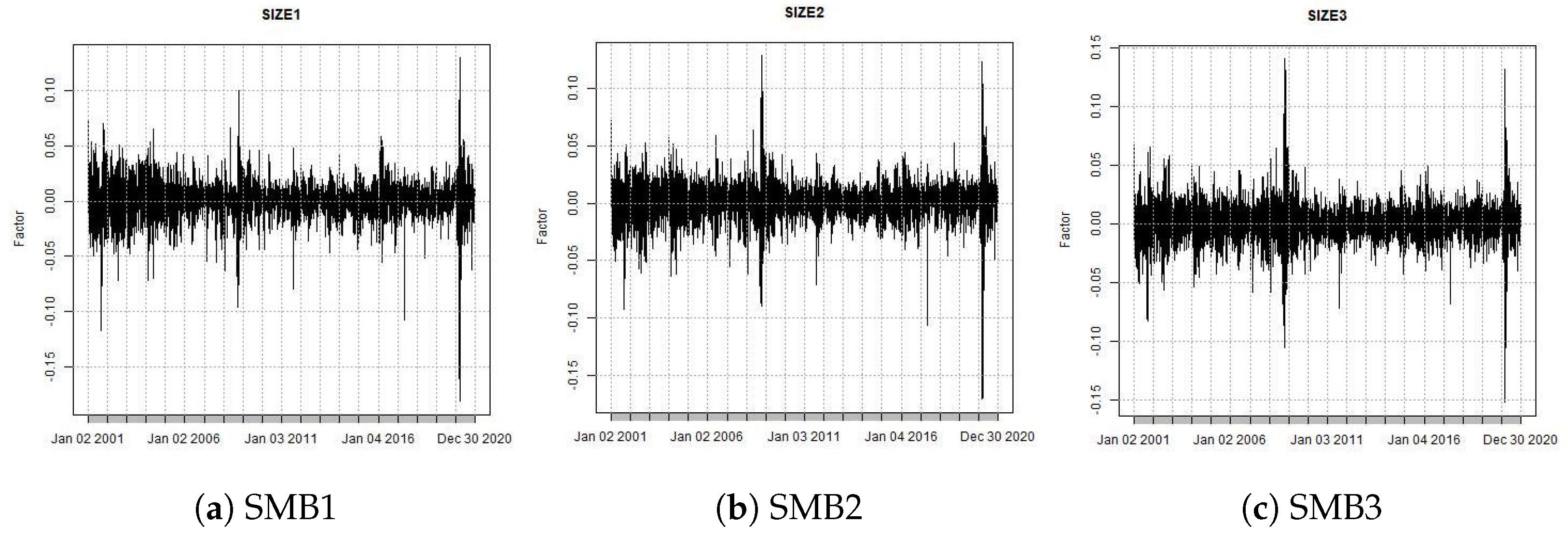
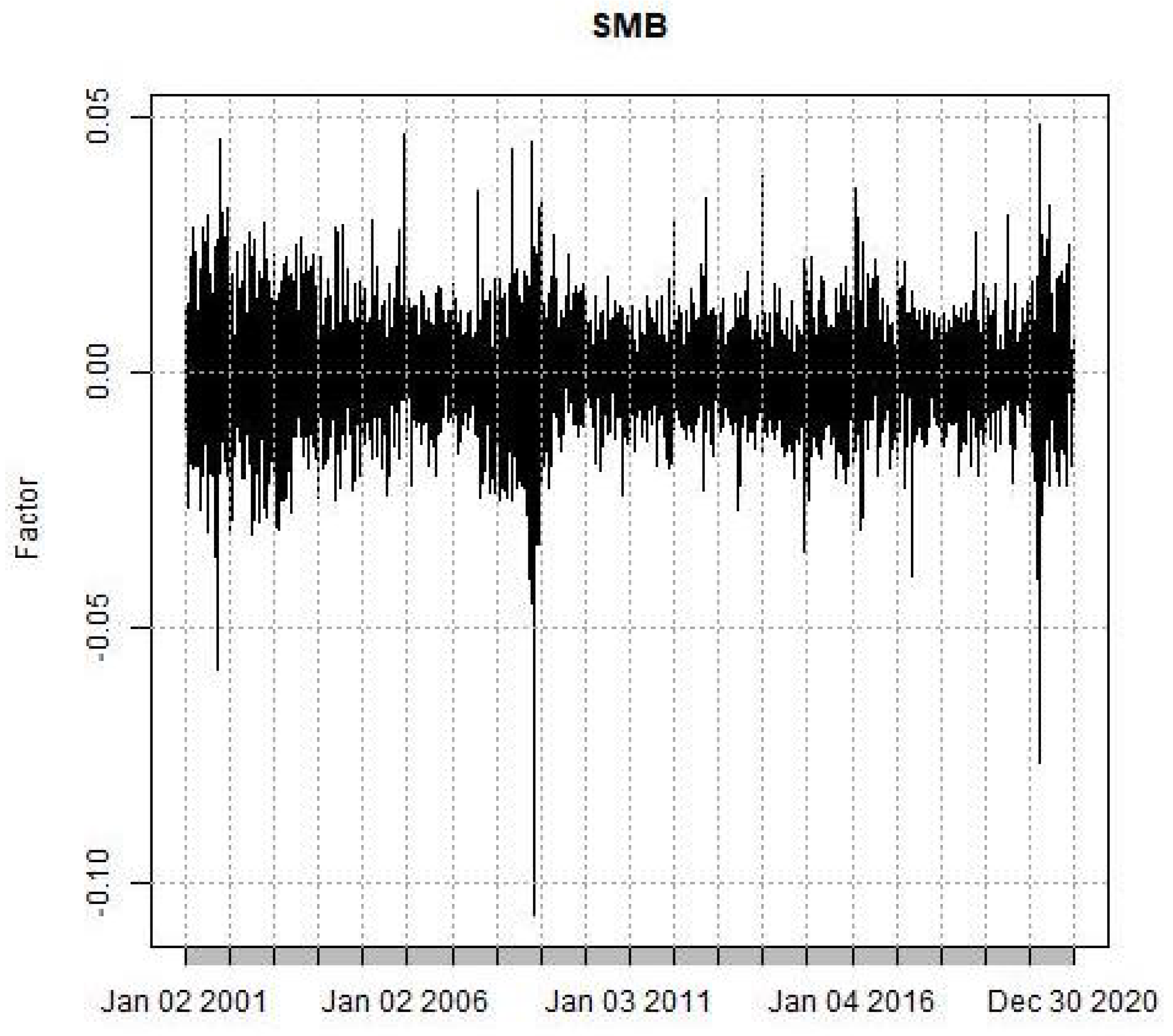
The size factor $SMB$ (small (− big) is the return of a portfolio long on stocks with low market capitalization (smal) and short stocks with high market capitalization (big’). Every January of the year t, the shares are classified as eligible according to the market capitalization of December of the year $t-1$, and are sorted and separated into three quantiles (portfolios). Then, the returns of the first portfolio (small’) and the third portfolio (big’) are calculated with equal weight. The $SMB$ factor is the return of the small portfolio minus the return of the big’ portfolio. Figure 2 shows the size factor returns.

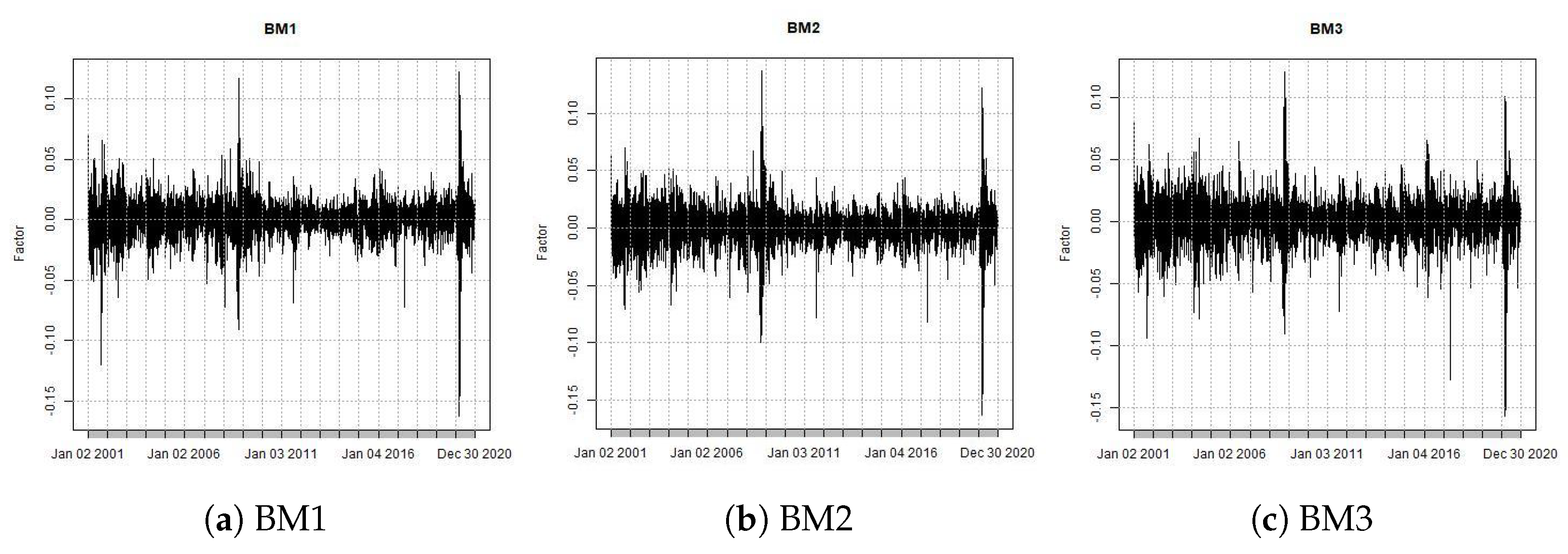
The factor related to BE/ME is the $HML$ factor (high minus low). This return is the return of a portfolio long on stocks with a high book-to-market ratio (high) and short on a low book-to-market ratio (low’). Every January of the year t, the shares are classified as eligible and sorted into three quantiles (portfolios) according to the firm’s book-to-market ratio in June of the year $t-1$. Again, equal weighted returns of the high portfolio minus the returns of the low portfolio are constructed. Figure 3 presents the book-to-market factor returns.

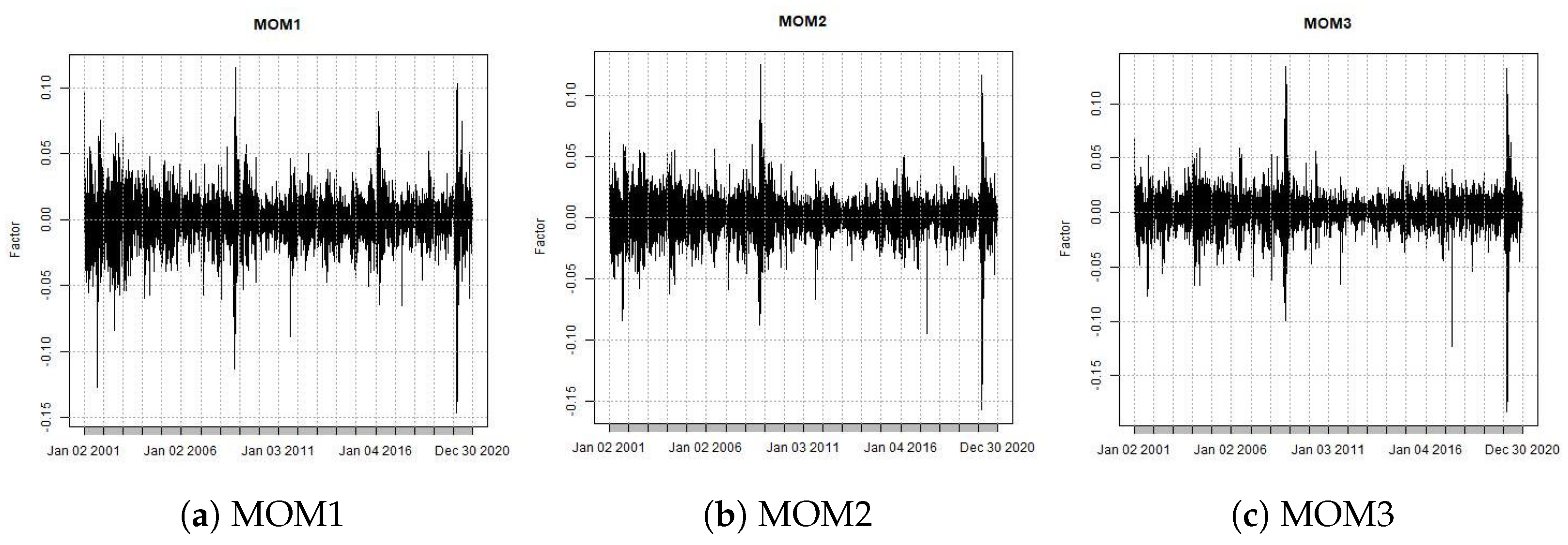
The $WML$ factor (winners minus losers) is the return of a portfolio long on stocks with high past returns (winners) and short on low past returns (losers). Every month, t shares are classified as eligible and divided into three quantiles (portfolios) according to their cumulative returns between the months $t-12$ and $t-2$, with equal weighted returns of the first portfolio (losers) and the third portfolio (winners’). The $WML$ factor is the return of the winners’ portfolio minus the return of the losers’ portfolio. The returns of $WML$ factor are shown in Figure 4.

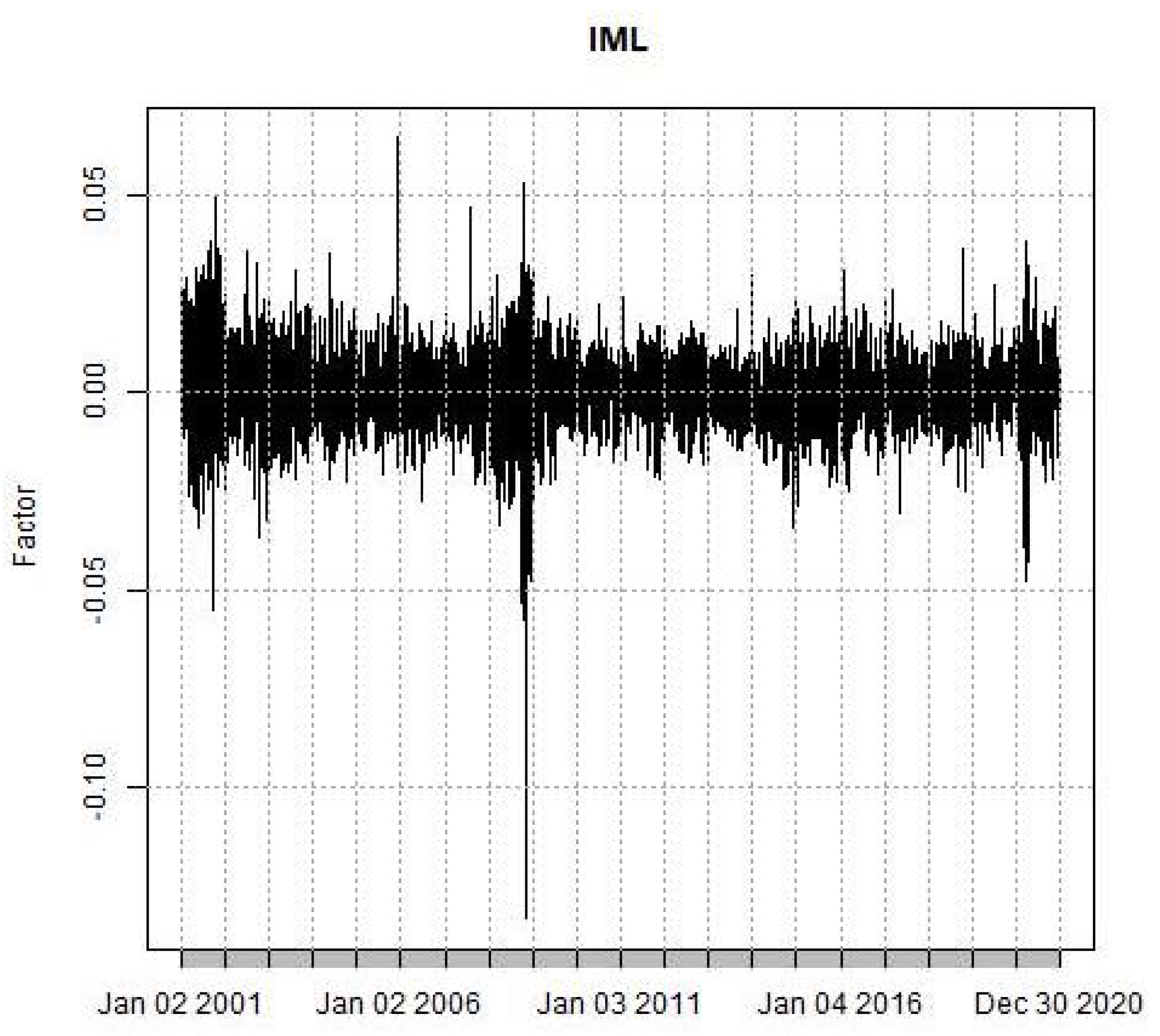
The $IML$ factor (illiquid minus liquid) is the return of a portfolio long on highly illiquid stocks (Illiquid’) and short on low illiquid (Liquid’). Every t month, we sort eligible stocks (in ascending order) into three quantiles (portfolios) according to the moving average of illiquidity over the previous twelve months (stock illiquidity is calculated according to Acharya and Pedersen (2002) method). As with the previous factors, we calculated with equal weight the returns of the first portfolio (liquid) and the third portfolio (illiquid). The factor $IML$ is the return on the illiquid’ portfolio minus the return on the liquid’ portfolio. Figure 5 presents the book-to-market factor returns.

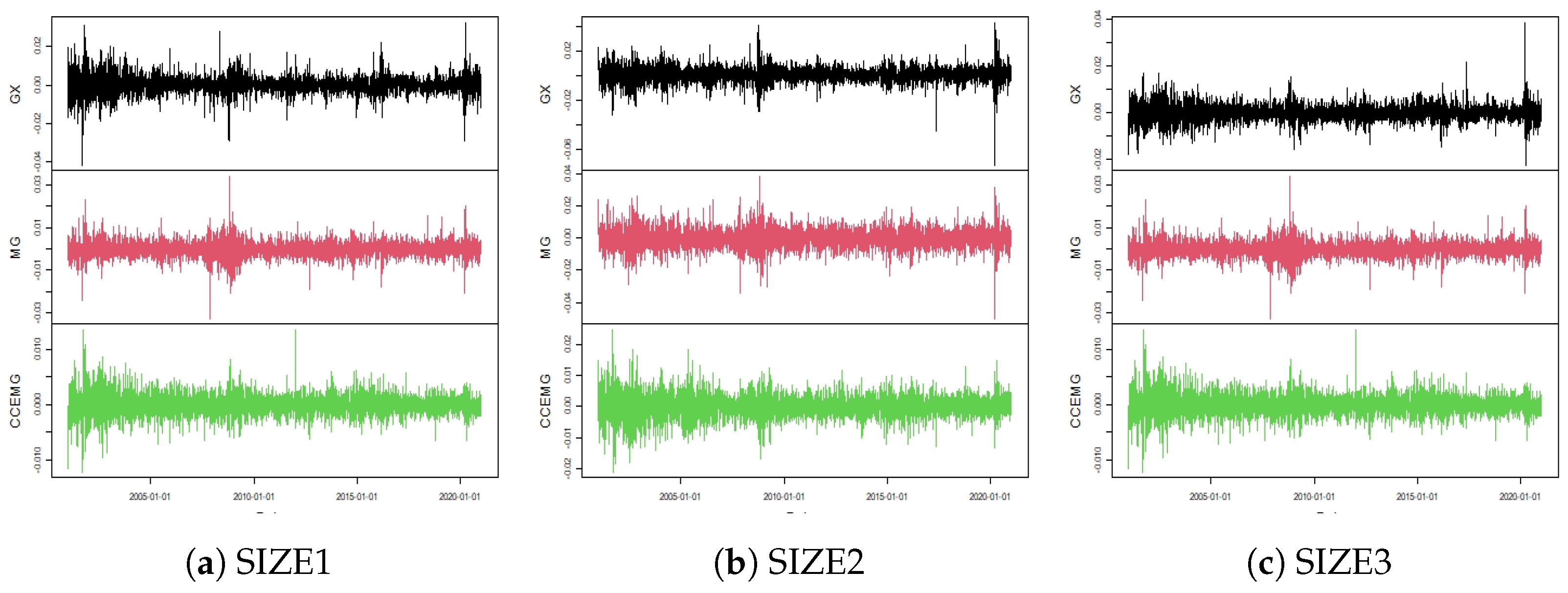
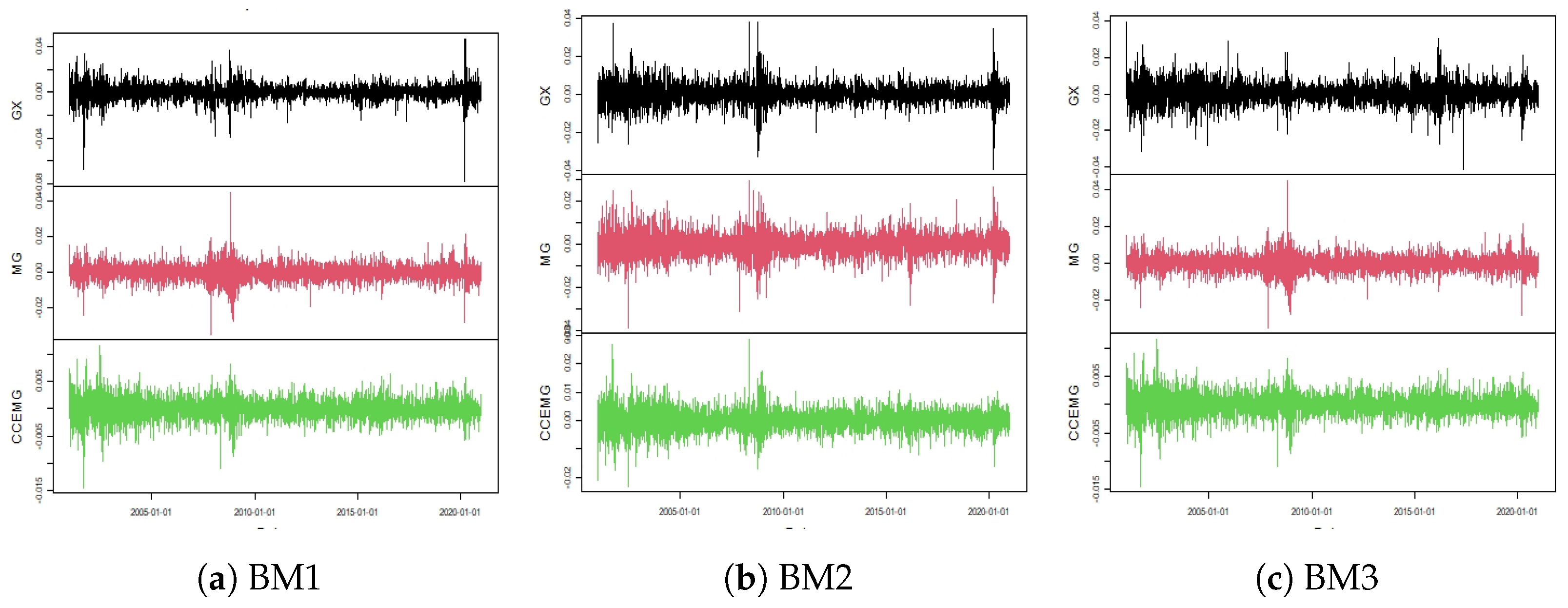
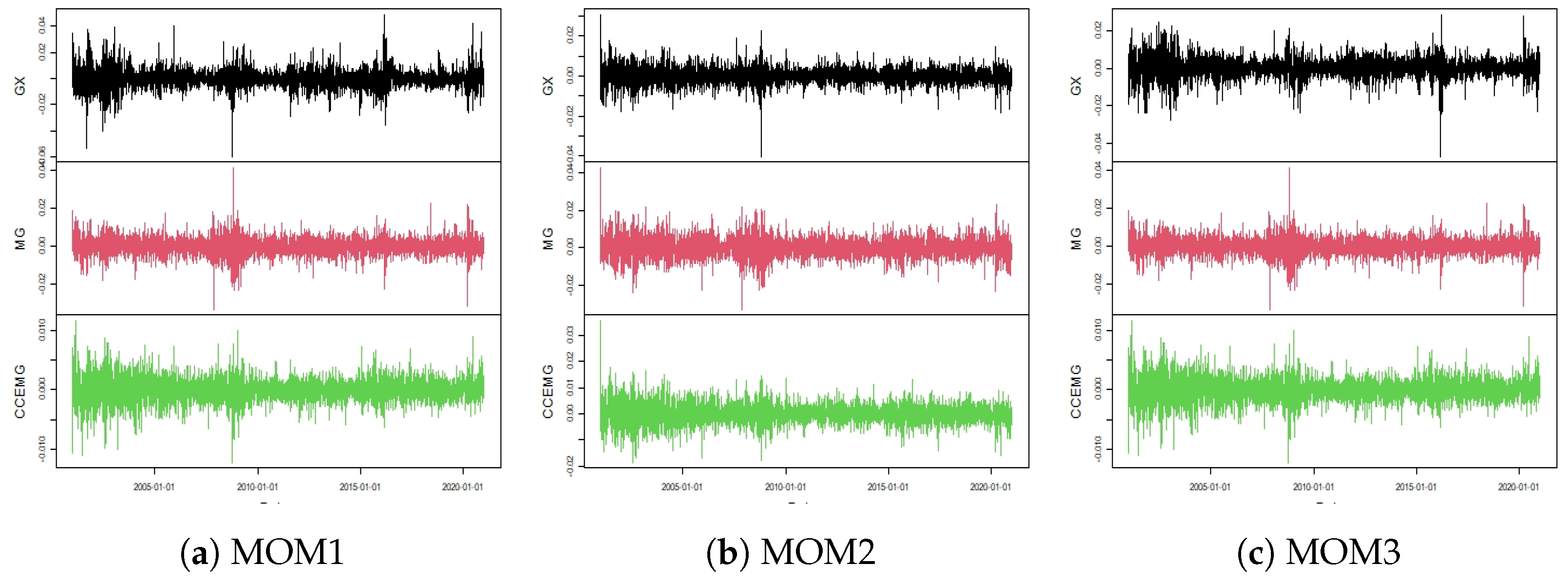
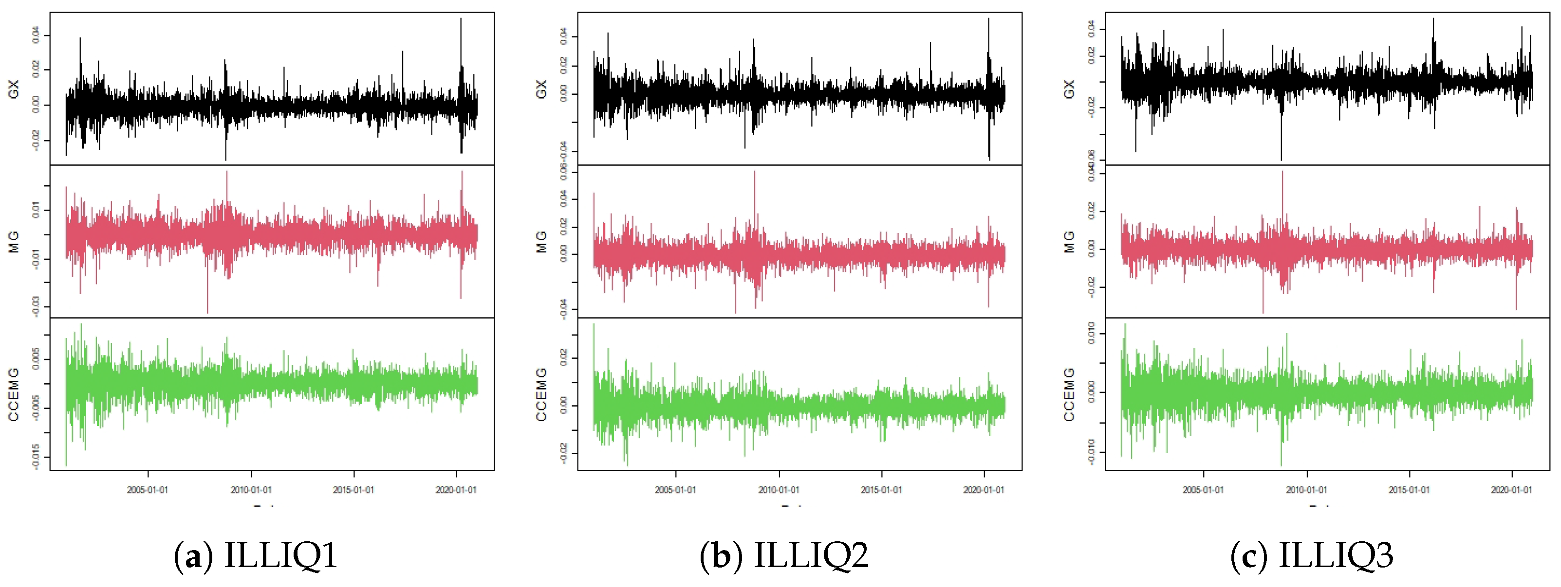
The dependent variables in our analysis are asset portfolios constructed using sorting by asset characteristics. The use of portfolios as dependent variables is a way of summarizing the heterogeneity observed in market assets, eliminating the idiosyncratic effects observed in individual assets by the diversification mechanism. The 12 portfolios returns analyzed are divided into four groups:

• Three portfolios sorted by size;
• Three portfolios classified by book-to-market;
• Three portfolios sorted by momentum;
• Three portfolios classified by illiquidity.

Portfolios sorted by size are obtained as follows: every January of year t, eligible stocks are sorted in ascending order into terciles according to their market capitalization in December of year $t-1$. Then, the portfolios are held for the year t. Portfolios sorted by book-to-market are similar: every January of the year t, eligible stocks are sorted in ascending order in terciles, according to the ratio between the book value and market value in June of the year $t-1$. Then, the portfolios are held for the year t.

Momentum sorted portfolios are constructed in a similar way: every month t, eligible stocks are sorted in ascending terciles according to their cumulative returns for month $t-12$ and month $t-2$, and are held for the month t. Finally, the portfolios sorted by illiquidity are sorted in ascending terciles according to the moving average of the illiquidity of the twelve previous months, according to Acharya and Pedersen (2002), and again are held for the year t.

In order to be considered eligible, the stock shares traded on BOVESPA had to meet three criteria: The share is the company’s most traded share (that is, the one with the highest volume traded during the last year); the shares were traded in more than $80\%$ of the days of the year $t-1$, with a volume greater than BRL 500,000.00 per day, and if the share was listed in the year $t-1$, the period considered runs from the day of listing to the last day of the year; the shares were initially listed before December of the year $t-1$.

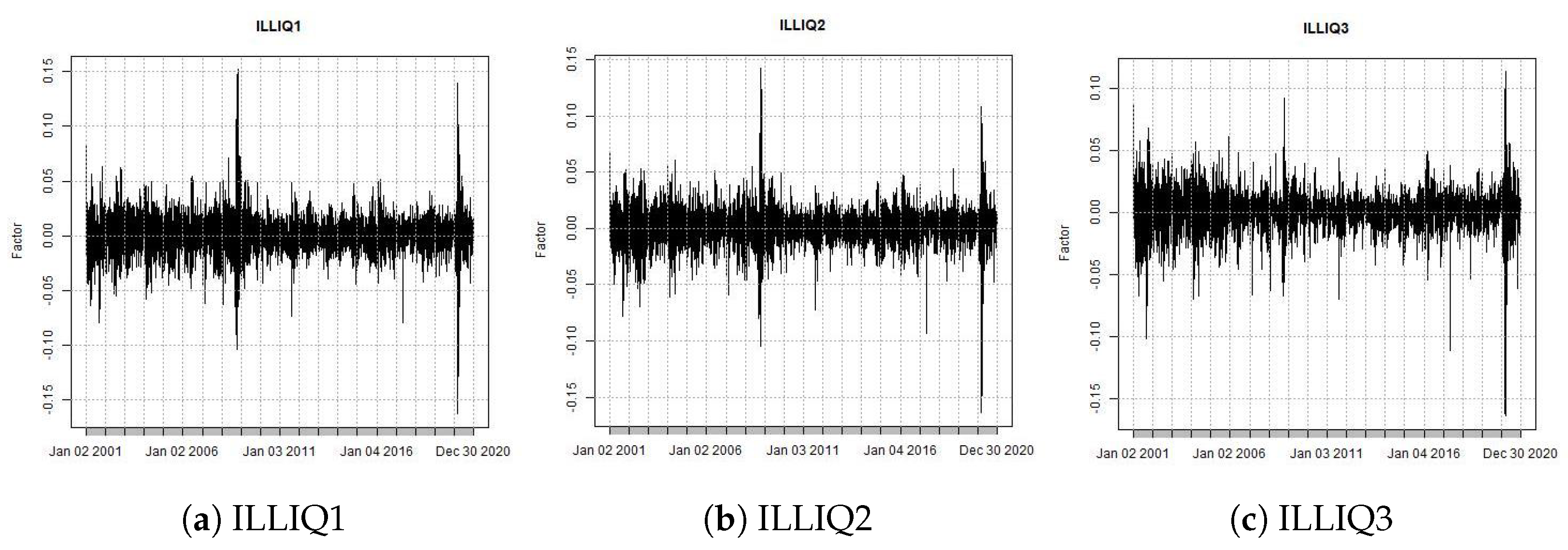
Figure 6, Figure 7, Figure 8 and Figure 9 show the returns of analyzed portfolios, and

Table 1. Descriptive statistics.

	Mean	SD	Skewness	Kurtosis	Min	Max
Rm-rf	0.0002	0.0160	−0.2439	11.6293	−0.1473	0.1411
SMB	−0.0000	0.0097	−0.4258	8.5887	−0.1061	0.0484
HML	0.0002	0.0090	0.0165	6.2645	−0.0609	0.0655
WML	0.0006	0.0107	−0.2708	6.7720	−0.0851	0.0660
IML	0.0001	0.0099	−0.5250	11.8186	−0.1333	0.0643
Port_Size1	0.0007	0.0166	−0.8413	13.2969	−0.1813	0.1297
Port_Size2	0.0007	0.0162	−0.7469	14.7212	−0.1518	0.1284
Port_Size3	0.0007	0.0158	−0.1905	12.4805	−0.1518	0.1403
Port_BM1	0.0006	0.0151	−0.7756	15.9295	−0.1630	0.1220
Port_BM2	0.0007	0.0159	−0.6090	13.6556	−0.1631	0.1365
Port_BM3	0.0008	0.0171	−0.5011	9.8070	−0.1575	0.1208
Port_MOM1	0.0004	0.0175	−0.4444	9.0643	−0.1467	0.1151
Port_MOM2	0.0008	0.0157	−0.4945	12.0702	−0.1576	0.1254
Port_MOM3	0.0009	0.0158	−0.8577	19.4689	−0.1832	0.1337
Port_ILLIQ1	0.0006	0.0173	−0.1605	12.1724	−0.1628	0.1518
Port_ILLIQ2	0.0009	0.0163	−0.4942	12.2508	−0.1639	0.1420
Port_ILLIQ3	0.0006	0.0158	−0.7831	13.0073	−0.1635	0.1130

presents the descriptive statistics for the risk factors and portfolios analyzed.

5. Results

5.1. Wald Tests for MG and CCE Estimators

The first step to perform the Wald tests was to calculate the coefficients of each of the estimators for the model (1). In

Table 2. MG estimator results.

	${\mathit{R}}_{\mathit{m}}-{\mathit{r}}_{\mathit{f}}$	$\mathit{SMB}$	$\mathit{HML}$	$\mathit{IML}$	$\mathit{WML}$
Parameter	$0.9548$	$0.2987$	$0.0121$	$0.0653$	$-0.0511$
Std. Dev.	$0.0041$	$0.0644$	$0.0623$	$0.0641$	$0.0617$
t-stat	$236.5998$	$4.6361$	$0.1934$	$1.0192$	$-0.8270$
$R^2$	$0.91133$

Note: Results were obtained by calculating the MG estimator for a panel with $nxT$, where $n=12$ and $T=4950$, which results in a total of 59,400 observations.

, we present the results obtained for the mean group estimator. We observe that, for this estimator, the t-statistics indicate the statistical significance of the market and size factors for the panel structure of returns. In addition, the estimated $R^2$ for the model was approximately 0.91133, pointing to a relevant fit to the systematic variation on the observed returns.

In

Table 3. CCE estimator results.

	${\mathit{R}}_{\mathit{m}}-{\mathit{r}}_{\mathit{f}}$	$\mathit{SMB}$	$\mathit{HML}$	$\mathit{IML}$	$\mathit{WML}$
Parameter	$0.0918969$	$1.2449408$	$0.1621465$	$0.0074829$	$-0.1936320$
Std. Dev.	$0.1189371$	$0.8526953$	$0.1179169$	$0.3221000$	$0.1493925$
t-stat	$0.7727$	$1.4600$	$1.3751$	$0.0232$	$-1.2961$
$R^2$	$0.97151$

Note: The above results were obtained by calculating the CCE-MG estimator for a panel with $nxT$, where $n=12$ and $T=4950$, which results in a total of 59,400 observations.

, we present the results of the CCE estimator for the model (1), and in

Table 4. Wald tests for factor sufficiency.

	Chisq	Pr (>Chisq)
Test	434.53	0.00
Test 2	49,066.00	0.00
Test 3	601.36	0.00
Test 4	566.76	0.00

Note: This test consists of Wald tests for the equality of parameters for the MG and CCE panel estimators. Test 1 constructs the Wald test statistic using the estimated parameters and covariance parameter matrix from the MG estimation, and assuming the null hypothesis in which the MG parameter is equal to the point parameter values estimated by the CCE method. Test 2 inverts the construction of the Wald statistic, using the estimated parameters and covariance parameter matrix from the CCE estimation, and assuming the null hypothesis that the CCE parameter is equal to the point parameter values estimated by the MG method. Test 3 uses a Hausman form, using the difference between the covariance matrices as a covariance matrix to form the MG and CCE estimators. Test 4 tests the equality of variances between the MG and CCE estimations.

, we present the results of the Wald test with the null hypothesis that the coefficients are equal to the coefficients obtained by the mean group estimator. We can observe a significant variation of the parameters of the CCE estimation compared to the MG estimation, indicating the presence of omitted relevant factors in the estimation.

As explained in Section 3.1.3, we performed four Wald tests. In Test 1, we performed a Wald test using the estimated parameters from the MG estimator and assuming a null hypothesis, in which the parameters are equal to the estimated parameters obtained with the CCE estimator and used in the Wald test, the estimated covariance parameter matrix is estimated using the MG method. We can see that Test 1 rejects the null hypothesis. In Test 2, we invert the models—we assume that, in the null hypothesis, the parameters estimated using the CCE method are equal to the parameter estimated from the MG estimator, using the estimated covariance matrix structure of the CCE estimator. We note in Table 4 that Test 2 also rejects the null hypothesis. Test 3 uses the difference between the covariance matrices from the MG and CCE estimators as the covariance matrix in the test, considering the uncertainty associated with parameter estimation in both models and being equivalent to a Hausman (1978) test, and again rejects the null hypothesis. Test 4 presents the test comparing the equality of variances of the two estimations. It also again rejects the null hypothesis. With this, we conclude that there are strong indications that the model has omitted factors.

5.2. Applying the GX Method for Brazilian Market Portfolios

The estimator proposed by Giglio and Xiu (2021) fundamentally depends on determining the number of principal components used in implementing the correction for the risk factors omitted in the model, and therefore, we need an estimator for ${\widehat{p}}_1^2$. To determine this number of components, some metric of the optimal choice of the number of factors must be used. To verify the impact of this choice, in the appendix of the work, we present a simulation analysis comparing several choice functions for the number of latent factors, for various combinations of factors, assets, and sample sizes.

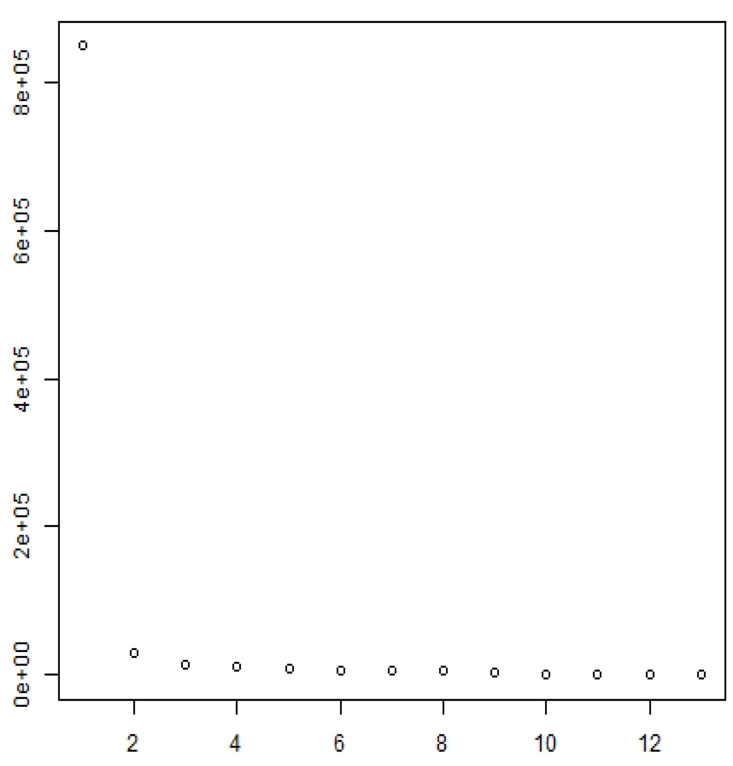
The results of the simulation analysis presented in the Appendix helped us choose the ${\widehat{p}}_1^2$ estimator. After this choice, the first step was to calculate the PCA of the matrix ${\left(NT\right)}^{-1}{\overline{R}}^{\prime }\overline{R}$. With the eigenvalues obtained by PCA, we calculate the ${\widehat{p}}_1^2$ estimator. For our portfolios ${\widehat{p}}_1^2=2$, defined using the criteria discussed in the Appendix, that is, assuming that two omitted latent factors influence our estimation. Figure 10 shows the 12 first eigenvalues obtained by PCA.

With this choice of ${\widehat{p}}_1^2$, we estimate $\widehat{\beta }$ and $\widehat{V}$. Both are used to obtain the $\widehat{\gamma }$ risk premium.

Table 5. Fama–MacBeth and Giglio–Xiu estimated risk premium.

	FM $\widehat{\mathit{\gamma }}$	FM $\widehat{\mathit{\gamma }}$ SD	GX $\widehat{\mathit{\gamma }}$	GX $\widehat{\mathit{\gamma }}$ SD	${\mathit{R}}^2\mathbf{GX}$
Intercept	0.00442	0.00121	0.00135	0.00092
Rm-rf	−0.00387	0.00128	−0.00060	0.00092	0.930
SMB	−0.00005	0.00014	−0.00014	0.00018	0.810
HML	0.00026	0.00013	−0.00013	0.00014	0.183
WML	0.00056	0.00015	0.00014	0.00015	0.283
IML	0.00006	0.00014	−0.00002	0.00021	0.769

reports the risk premium estimates uncorrected for the presence of omitted factors using the Fama–MacBeth (Fama and Macbeth (1973)) approach and the risk premium estimated using the GX correction for each systematic risk factor, and also the $R^2$ between the original and corrected factors. We can observe the relevant changes in the estimation of the risk premium after the GX correction, including the changes in the sign of the risk premium for HML and IML, and a lesser explained variance for the HML and WML factors using the GX approach.

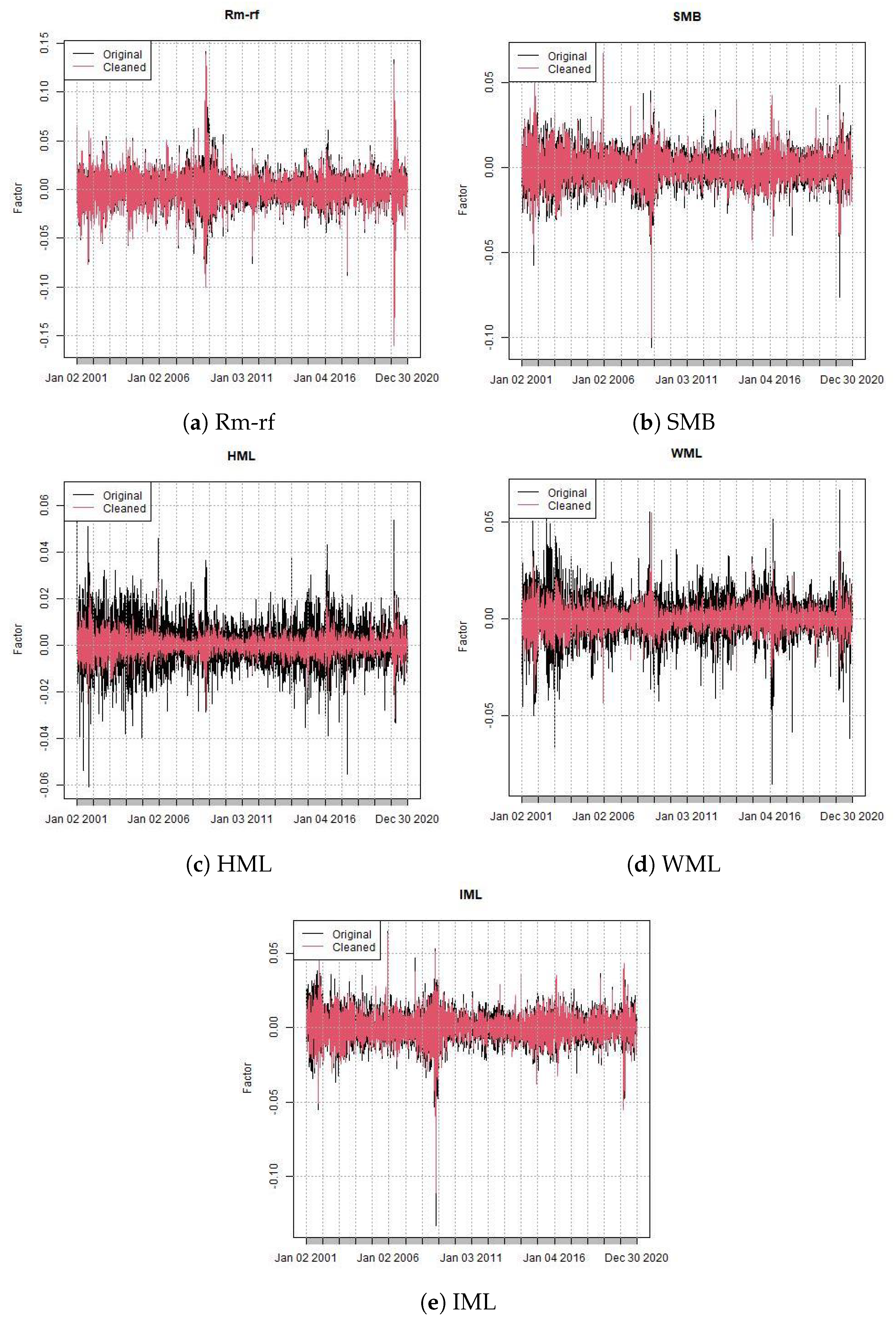
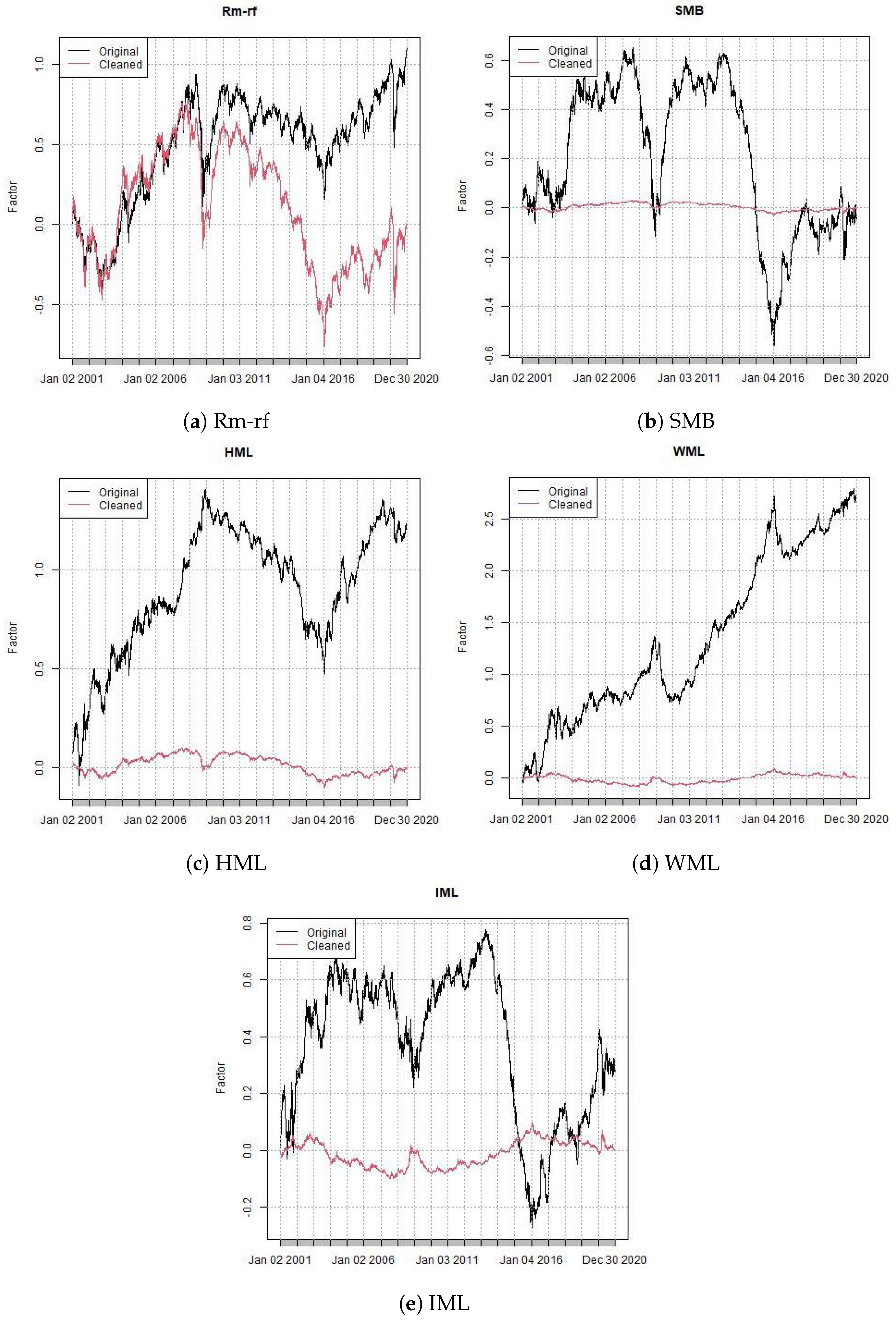
Figure 11 shows the original and cleaned risk factors using the GX approach, and Figure 12 shows the accumulated values of these factors. We can observe that the cleaned factors present a much lower variation than the original factors, which explains the estimated differences for the estimated risk premiums.

5.3. Comparison of the MG, CCE, and GX Estimators

To compare the performance of the three methods (MG, CCE, and GX) in explaining the systematic variation observed in returns, we will compare the fit of these models to the observed returns, using the residuals estimated for each portfolio, defined by:

$$\begin{array}{c}\hfill {\widehat{e}}_{it}=R_{it}-{\widehat{R}}_{it}\end{array}$$

(45)

where $R_{it}$ is the return on portfolio i for period t and ${\widehat{R}}_{it}$ is the estimated return on portfolio i for period t by each method (MG, CCE, and GX).

The residual series were used to calculate the following metrics:

• Mean:

  $$\begin{array}{c}\hfill {\overline{e}}_i=\frac{1}{N}\sum _{t=1}^T{\widehat{e}}_{it}\end{array}$$

  (46)
• Standard deviation:

  $$\begin{array}{c}\hfill {\sigma }_i={\left(\sum _{t=1}^T\frac{{(\widehat{e}-{\overline{e}}_{it})}^2}{N}\right)}^{1/2}\end{array}$$

  (47)
• Mean squared error (MSE):

  $$\begin{array}{c}\hfill MS{E}_i=\frac{1}{N}\sum _{t=1}^T{\widehat{e}}_{it}^2\end{array}$$

  (48)

  where, N = 12, that is, the number of portfolios and T = 4950, which is the number of periods.

In

Table 6. Residuals for NEFIN portfolios.

Portfolio	Model	Min	Max	Mean	Std. Dev.	MSE
SIZE1	GX	−0.0416	0.0325	0.0000	0.0047	0.000023
SIZE1	MG	−0.0327	0.0342	0.0000	0.0038	0.000015
SIZE1	CCE	−0.0122	0.0135	0.0000	0.0019	0.000004
SIZE2	GX	−0.0726	0.0429	0.0002	0.0065	0.000042
SIZE2	MG	−0.0501	0.0388	0.0000	0.0062	0.000039
SIZE2	CCE	−0.0212	0.0247	0.0000	0.0037	0.000014
SIZE3	GX	−0.0225	0.0387	−0.0001	0.0036	0.000013
SIZE3	MG	−0.0327	0.0342	0.0000	0.0038	0.000015
SIZE3	CCE	−0.0122	0.0135	0.0000	0.0019	0.000004
BM1	GX	−0.0778	0.0472	0.0002	0.0068	0.000047
BM1	MG	−0.0346	0.0448	0.0000	0.0044	0.000019
BM1	CCE	−0.0145	0.0116	0.0000	0.0019	0.000004
BM2	GX	−0.0392	0.0381	0.0001	0.0051	0.000026
BM2	MG	−0.0385	0.0294	0.0000	0.0053	0.000028
BM2	CCE	−0.0232	0.0286	0.0000	0.0037	0.000014
BM3	GX	−0.0410	0.0396	0.0002	0.0055	0.000030
BM3	MG	−0.0346	0.0448	0.0000	0.0044	0.000019
BM3	CCE	−0.0145	0.0116	0.0000	0.0019	0.000004
MOM1	GX	−0.0597	0.0491	−0.0002	0.0073	0.000053
MOM1	MG	−0.0332	0.0412	0.0000	0.0045	0.000021
MOM1	CCE	−0.0123	0.0117	0.0000	0.0020	0.000004
MOM2	GX	−0.0330	0.0427	0.0000	0.0053	0.000028
MOM2	MG	−0.0400	0.0308	0.0001	0.0040	0.000016
MOM2	CCE	−0.0186	0.0355	0.0000	0.0037	0.000014
MOM3	GX	−0.0471	0.0287	0.0001	0.0053	0.000028
MOM3	MG	−0.0332	0.0412	0.0000	0.0045	0.000021
MOM3	CCE	−0.0123	0.0117	0.0000	0.0020	0.000004
ILLIQ1	GX	−0.0305	0.0496	−0.0003	0.0051	0.000026
ILLIQ1	MG	−0.0322	0.0261	0.0000	0.0042	0.000018
ILLIQ1	CCE	−0.0168	0.0122	0.0000	0.0022	0.000005
ILLIQ2	GX	−0.0457	0.0533	−0.0001	0.0064	0.000041
ILLIQ2	MG	−0.0420	0.0609	0.0000	0.0064	0.000042
ILLIQ2	CCE	−0.0248	0.0346	0.0000	0.0041	0.000017
ILLIQ3	GX	−0.1681	0.1139	0.0007	0.0156	0.000244
ILLIQ3	MG	−0.0322	0.0261	0.0000	0.0042	0.000018
ILLIQ3	CCE	−0.0168	0.0122	0.0000	0.0022	0.000005

, we present the results obtained for the portfolios. We note that, in general, the MG and CCE residual estimators have a mean closer to zero compared to the GX estimator. The best results in the mean squared error criterion are obtained by the CCE method for all portfolios, and the residuals constructed by MG estimators also dominate the GX approach in the MSE criterion, except for SIZE3, BM2, and ILLIQ2 portfolios.

These results indicate that, among the three methods used to explain the systematic variation observed in the market returns, the CCE method presents the overall best performance in the MSE metric, whilst simultaneously, there are weights bias and variance in estimates, and the GX estimator appears to introduces additional noise in the estimation of expected returns when correcting for the presence of factors omitted in the estimation. The CCE estimator also performs better in relation to extreme values/outliers observed in the data, since the residuals estimated by this method present the least extreme residuals in terms of the maximum and minimum values.

Figure 13, Figure 14, Figure 15 and Figure 16 show the time series of residuals constructed by each method for size, book-to-market, moment and illiquidity portfolios.

6. Conclusions

In this study, we investigate the applicability of the Fama–French five-factor model in explaining expected returns within the Brazilian asset market. Our analysis takes into account the potential consequences of omitting relevant factors in the model specification. To address this concern, we employ two distinct analytical approaches. Firstly, we construct a Wald test to assess the presence of omitted factors, examining both the temporal and cross-sectional dimensions of the data. To achieve this, we utilize two panel data estimators. Specifically, we compare the parameter estimates from the mean group (MG) estimator (Pesaran and Smith 1995), which does not correct for omitted factors, with those from the common correlated effects (CCE) estimator (Pesaran 2006), which accounts for omitted factors/variables in panel data estimations. Our findings reject the null hypothesis of parameter equality between the two estimations, strongly suggesting the existence of omitted factors in our estimation of the Fama–French five-factor model within the Brazilian stock market data.

With the identification of these omitted factors, we adopt the estimator introduced by Giglio and Xiu (2021). This approach enables us to estimate the risk premium associated with the observed factors while considering the potential presence of omitted factors and measurement errors. Subsequently, we compare the risk premiums for the included factors estimated using this correction with those derived from the uncorrected Fama–MacBeth estimation. This comparison reveals substantial differences between the parameters estimated under these two specifications, further emphasizing the significance of omitted factors in risk premium estimation.

Furthermore, we conduct a comparative analysis of three models: MG, CCE, and GX. We assess their predictions for the expected returns of the portfolios under scrutiny by calculating predicted returns and evaluating the residuals generated by each model. Our results indicate that the CCE estimator offers the most accurate predictions for expected returns, as it exhibits the lowest mean squared error. Additionally, this suggests that the correction proposed by Giglio and Xiu (2021) is less precise in estimating the expected returns compared to the panel estimation based on common correlated effects.

The core premise of the Giglio and Xiu (2021) approach hinges on the belief that the underlying data-generating process (DGP) for returns is influenced by latent but strong factors, and the PCA can uncover all the pivotal pricing factors. They posit that these latent factors can be discovered through principal component analysis (PCA). This issue carries significant weight, especially in light of the extensive assortment of factors and test assets found in financial literature, as it is quite plausible that within any cross-section of the test assets, some factors may prove to be weak rather than strong. The prevalence of this weak factor problem is evident in empirical data. Lettau and Pelger (2020) shows that employing weak factors in addition to those identified by PCA yields significantly better out-of-sample performance compared to models that solely rely on PCA-identified factors, and show that PCA-based factors often overlook low volatility components with high Sharpe ratios, a crucial aspect in asset pricing.

Onatski (2012) explores the utilization of principal component estimation in the context of large-factor models featuring weak factors. He emphasizes a crucial point: when a factor does not explain a substantial portion of the variance in the data, PCA cannot detect it. Additionally, Pesaran and Smith (2019) delve into the ramifications of factor strength and pricing errors when estimating risk premiums. They observe that the conventional two-pass risk premium estimation method exhibits a slower convergence as factors lose their strength. Even if all factors are robust, the presence of highly correlated factors can introduce the challenge of the weak factor problem.

The superior performance of the CCE estimator compared to the GX estimator can be attributed to the findings of Chudik et al. (2011), who demonstrated that, when weak or semi-strong factors are present, the principal component estimates of factors may lack consistency. In contrast, the CCE estimator exhibits good performance and minimal size distortions. Notably, this issue does not impact the CCE estimator, as its objective does not revolve around achieving consistent factor estimation. Instead, it addresses error cross-section dependence more broadly by employing cross-section averages to mitigate such effects. A similar interpretation of the relative performance of estimators based on cross-sectional averages compared to principal component-based estimators can be found in Westerlund and Urbain (2015) and Kapetanios et al. (2021), which is in violation of the assumptions necessary for estimating principal components, whilst CCE estimators tend to have better performance and the robustness properties of CCE analyzed by Chudik and Pesaran (2015) are valid.

We also evaluated in the Appendix of the work in which the estimator of the number of factors proposed by Giglio and Xiu (2021) uses four penalty functions. Although all penalty functions approach zero as N and T increase, we were unable to identify a penalty function that satisfies the second condition and accurately estimates the factors in our simulations. Despite this limitation, we found that the Giglio and Xiu (2021) estimator performed well with three of the penalty functions, particularly in simulations with one or three factors.

It is important to emphasize that our analysis and the estimation methods used depend on some important assumptions that may be violated. An essential assumption for the application of the panel estimators (MG and CCE) used as well as the GX estimator is a linear structure of dependence between the assets. We are assuming a linear pricing model based on the arbitrage price structure theory and a stochastic discount factor with a linear structure. Although it is a common assumption in this literature and especially in practical applications, it is important to note that there may be evidence contrary to this assumption.

For example, a non-linear dependence structure may occur in periods of market stress, where the occurrence of an extreme event in a series is non-linearly related to extremes in other processes, which would be a violation of the linear dependence between assets. Although the use of portfolios both in defining dependent variables and in constructing portfolio risk factors minimizes this problem through diversification, it is important to note that we may still be subject to problems such as nonlinear tail dependencies and other similar dependency structures. As we can observe the occurrence of extreme events and outliers both in the original series and in the estimation residuals, we cannot guarantee the existence of a multivariate normality structure, which would guarantee a linear dependence structure between assets. In this aspect, the estimators used implicitly depend on the assumption of linearity and/or joint multivariate normality. Similarly, other violations, for example, the non-sphericity in the covariance matrix (see, e.g., Baltagi et al. 2015), can also affect the finite sample properties of our estimators, since the existence of conditional volatility in financial time series generates heavy-tailed distributions, and harms the efficiency properties of estimators in finite samples.

Although there is a literature on estimating nonlinear panel models using the general structure of common correlated effects and mean group estimators (e.g., Hacıoğlu Hoke and Kapetanios 2021; Chen and Zhang 2023) and similar corrections to principal component-based estimators (Chen et al. 2014), these estimators require the nonlinear functional form linear is known, which is not the case in our problem. An alternative approach would be, for example, to use a copula structure, where we could define the nonlinear dependence function through some copula function with nonlinear tail dependence, which would be a very interesting extension of our analysis. We recognize that our analysis depends on a linear pricing structure, and that specification issues such as the rejection of normality, nonlinear dependence, and problems with extreme values can affect our results and conclusions. An analysis of the robustness properties of the Wald tests for factor sufficiency and MG, CCE, and GX estimators analyzed in the present paper in relation to these mis-specification problems in the estimation of risk premia is an interesting extension of the analyses carried out in our work.

As a general conclusion, our analyses show that the use of econometric corrections for omitted factors is important for estimating the risk premium in the Brazilian financial market, and that the correction method used is also relevant.

All factor sufficiency tests performed conclusively indicate the presence of omitted factors when using the five factors constructed by NEFIN to estimate risk premiums for portfolios constructed using sortings. As these portfolios serve as proxies for general stock portfolios in Brazil, we have relevant evidence about the need for additional risk factors and the use of robust econometric methods in estimating risk premiums in the Brazilian stock market.

Investment strategies and portfolio selection using factors depend directly on the accurate estimation of the risk premium associated with each factor, as discussed in Alles Rodrigues and Casalin (2022); Brière and Szafarz (2020); Caldeira et al. (2013), and thus the econometric properties of risk premium estimators are relevant in practical market applications. Our results indicate that the CCE estimator, which corrects the presence of omitted factors by exploring the averages through a panel structure, appears to estimate the risk premium structure for the analyzed portfolios in a less biased and accurate way, obtaining residuals with less variability and bias, and thus better performance in predicting the expected returns, an essential property in portfolio selection and risk measurement procedures.

References

1. Acharya, Viral V., and Lasse Heje Pedersen. 2002. Asset pricing with liquidity risk. Journal of Financial Markets 77: 31–56. [Google Scholar]
2. Alles Rodrigues, Alexandre, and Fabrizio Casalin. 2022. Factor investing in Brazil: Diversifying across factor tilts and allocation strategies. Emerging Markets Review 52: 100906. [Google Scholar] [CrossRef]
3. Araújo, Eurilton, Ricardo D. Brito, and Antonio Z. Sanvicente. 2021. Long-term stock returns in Brazil: Volatile equity returns for U.S.-like investors. International Journal of Finance & Economics 26: 6249–63. [Google Scholar] [CrossRef]
4. Bai, Jushan. 2003. Inferential theory for factors models of large dimensions. Econometrica 71: 135–71. [Google Scholar] [CrossRef]
5. Bai, Jushan, and Serena Ng. 2002. Determining the number of factors in approximate factors models. Econometrica 70: 191–221. [Google Scholar] [CrossRef]
6. Baltagi, Badi H., Chihwa Kao, and Bin Peng. 2015. On testing for sphericity with non-normality in a fixed effects panel data model. Statistics & Probability Letters 98: 123–30. [Google Scholar] [CrossRef]
7. Barasal Morales, Adriano, Márcio Laurini, and Anton Vrieling. 2023. Climate Risk Premium: Assessing the Influence of Global Warming Effects on Stock Market Dynamics. Technical Report. Rochester: SSRN. [Google Scholar] [CrossRef]
8. Bhatti, Madiha, and Abu Mirza. 2014. A comparative study of capm and seven factors risk adjusted return model. Paradigms 8: 13–25. [Google Scholar] [CrossRef]
9. Black, Fischer. 1972. Capital market equilibrium with restricted borrowing. Journal of Business 45: 444–55. [Google Scholar] [CrossRef]
10. Brière, Marie, and Ariane Szafarz. 2020. Good diversification is never wasted: How to tilt factor portfolios with sectors. Finance Research Letters 33: 101197. [Google Scholar] [CrossRef]
11. Bryzgalova, Svetlana, Jiantao Huang, and Christian Julliard. 2023. Bayesian solutions for the factor zoo: We just ran two quadrillion models. The Journal of Finance 78: 487–557. [Google Scholar] [CrossRef]
12. Caldeira, João F, Guilherme Valle Moura, and André Alves Portela Santos. 2013. Seleção de carteiras utilizando o modelo Fama-French-Carhart. Revista Brasileira de Economia 67: 45–65. [Google Scholar] [CrossRef]
13. Campbell, John Y., Andrew W. Lo, and A. Craig MacKinlay. 1997. The Econometrics of Financial Markets. Princeton: Princeton University Press. [Google Scholar]
14. Campiglio, Emanuele, Louis Daumas, Pierre Monnin, and Adrian von Jagow. 2023. Climate-related risks in financial assets. Journal of Economic Surveys 37: 950–92. [Google Scholar] [CrossRef]
15. Carvalhal, Marcelo Gonçalves Andre. 2017. Predicting Fama-French factors based on industry returns in Brazil. Corporate Ownership and Control 15: 44–51. [Google Scholar]
16. Chen, Liang, and Minyuan Zhang. 2023. Common correlated effects estimation of nonlinear panel data models. arXiv arXiv:2304.13199. [Google Scholar]
17. Chen, Mingli, Iván Fernández-Val, and Martin Weidner. 2014. Nonlinear panel models with interactive effects. arXiv arXiv:1412.5647. [Google Scholar]
18. Chen, Mingjing, and Jingzhou Yan. 2019. Unbiased cce estimator for interactive fixed effects panels. Economics Letters 75: 1–4. [Google Scholar] [CrossRef]
19. Cho, Cheol-Keun, and Bosung Jang. 2023. Durable consumption-based asset pricing model with foreign factors for the Korean stock market. International Journal of Financial Studies 11: 62. [Google Scholar] [CrossRef]
20. Chudik, Alexander, and M. Hashem Pesaran. 2015. Common correlated effects estimation of heterogeneous dynamic panel data models with weakly exogenous regressors. Journal of Econometrics 188: 393–420. [Google Scholar] [CrossRef]
21. Chudik, Alexander, M. Hashem Pesaran, and Elisa Tosetti. 2011. Weak and strong cross-section dependence and estimation of large panels. The Econometrics Journal 14: C45–C90. [Google Scholar] [CrossRef]
22. Cochrane, John H. 2005. Asset Pricing. Princeton: Princeton University Press. [Google Scholar]
23. Cochrane, John H. 2011. Presidential address: Discount rates. Journal of Finance 66: 1047–110. [Google Scholar] [CrossRef]
24. de Andrade Alves, Cássio Roberto, and Márcio Laurini. 2023. Estimating the Capital Asset Pricing Model with many instruments: A Bayesian shrinkage approach. Mathematics 11: 3776. [Google Scholar] [CrossRef]
25. De Vos, Ignace, and Joakim Westerlund. 2019. On cce estimation of factor-augmented models when regressors are not linear in the factors. Economics Letters 178: 5–7. [Google Scholar] [CrossRef]
26. Dirkx, Philipp, and Franziska J. Peter. 2020. The Fama-French five-factor model plus momentum: Evidence for the German market. Schmalenbach Business Review 72: 661–84. [Google Scholar] [CrossRef]
27. Fama, Eugene F., and Kenneth R. French. 1988. Dividend yields and expected stocks returns. Journal of Financial Economics 22: 3–25. [Google Scholar] [CrossRef]
28. Fama, Eugene F., and Kenneth R. French. 1992. The cross-section of expected stock returns. The Journal of Finance 47: 427–65. [Google Scholar]
29. Fama, Eugene F., and Kenneth R. French. 1993. Common risk factors in the returns on stocks and bonds. Journal of Financial Economics 33: 3–56. [Google Scholar] [CrossRef]
30. Fama, Eugene F., and Kenneth R. French. 1995. Size and book-to-market factors in earnings and returns. The Journal of Finance 50: 131–55. [Google Scholar]
31. Fama, Eugene F., and Kenneth R. French. 2015. A five-factors asset pricing model. The Journal of Financial Economics 116: 1–22. [Google Scholar] [CrossRef]
32. Fama, Eugene F., and James D. MacBeth. 1973. Risk, return, and equilibrium: Empirical tests. Journal of Political Economy 81: 607–36. [Google Scholar] [CrossRef]
33. Fang, Elaine, and Caio Almeida. 2019. Are higher-order factors useful in pricing the cross-section of hedge fund returns? Revista Brasileira de Finanças 17: 1–37. [Google Scholar] [CrossRef]
34. Fan, Jianqing, and Qiwei Yao. 2015. The Elements of Financial Econometrics, 1st ed. Cambridge, MA: Cambridge University Press. [Google Scholar]
35. Fan, Zhenzhen, Juan M. Londono, and Xiao Xiao. 2022. Equity tail risk and currency risk premiums. Journal of Financial Economics 143: 484–503. [Google Scholar] [CrossRef]
36. Faria Maciel, Claudia, Hudson Fernandes Amaral, Laíse Ferraz Correia, and Joyce Mariella Medeiros Cavalcanti. 2021. Performance of the Fama-French five-factor model in the pricing of anomalies in the Brazilian market. Revista Contemporânea de Contabilidade 18: 145–60. [Google Scholar]
37. Giglio, Stefano, and Dacheng Xiu. 2021. Asset pricing with omitted factors. Journal of Political Economy 129: 1947–90. [Google Scholar] [CrossRef]
38. Hacıoğlu Hoke, Sinem, and George Kapetanios. 2021. Common correlated effect cross-sectional dependence corrections for nonlinear conditional mean panel models. Journal of Applied Econometrics 36: 125–50. [Google Scholar] [CrossRef]
39. Harvey, Campbell R., and Guofu Zhou. 1990. Bayesian inference in asset pricing tests. Journal of Financial Economics 6: 221–54. [Google Scholar] [CrossRef]
40. Harvey, Campbell R., Yan Liu, and Heqing Zhu. 2015. … and the cross-section of expected returns. Review of Financial Studies 29: 5–68. [Google Scholar] [CrossRef]
41. Hausman, Jerry A. 1978. Specification tests in econometrics. Econometrica 46: 1251–71. [Google Scholar] [CrossRef]
42. Hou, Kewey, Chen Xue, and Lu Zhang. 2017. Replicating anomalies: An investment approach. Review of Financial Studies 28: 650–705. [Google Scholar] [CrossRef]
43. Hwang, Soosung, and Alexandre Rubesam. 2020. Bayesian Selection of Asset Pricing Factors Using Individual Stocks*. Journal of Financial Econometrics 20: 716–61. [Google Scholar] [CrossRef]
44. Kapetanios, George, Laura Serlenga, and Yongcheol Shin. 2021. Estimation and inference for multi-dimensional heterogeneous panel datasets with hierarchical multi-factor error structure. Journal of Econometrics 220: 504–31. [Google Scholar] [CrossRef]
45. Karabiyik, Hande, Jean-Pierre Urbain, and Joakim Westerlund. 2019. Cce estimation of factor-augmented regression models with more factors than observables. Journal of Applied Econometrics 34: 268–84. [Google Scholar] [CrossRef]
46. Kelly, Bryan, and Hao Jiang. 2014. Tail risk and asset prices. The Review of Financial Studies 27: 2841–71. [Google Scholar] [CrossRef]
47. Lettau, Martin, and Markus Pelger. 2020. Estimating latent asset-pricing factors. Journal of Econometrics 218: 1–31. [Google Scholar] [CrossRef]
48. Lintner, John. 1965. The valuation of risk assets and the selection of risky investments in stock portfolios and capital budgets. Review of Economics and Statistics 47: 13–37. [Google Scholar] [CrossRef]
49. Maharani, Astrid, and I. Made Narsa. 2023. Six-factor plus intellectual capital in the capital asset pricing model and excess stock return: Empirical evidence in emerging stock markets. Cogent Economics & Finance 11: 2252652. [Google Scholar] [CrossRef]
50. Málaga, Flávio Kezam, and José Roberto Securato. 2004. Aplicação do modelo de três fatores de Fama e French no mercado acionário brasileiro—Um estudo empírico do período 1995–2003. In Anais do Encontro Anual da ENANPAD. São Paulo: Universidade de São Paulo. [Google Scholar]
51. Malhotra, Davinder K., Tim Mooney, Raymond Poteau, and Philip Russel. 2023. Assessing the performance and risk-adjusted returns of financial mutual funds. International Journal of Financial Studies 11: 136. [Google Scholar] [CrossRef]
52. Markowitz, Harry. 1952. Portfolio selection. The Journal of Finance 7: 77–91. [Google Scholar]
53. McLean, R. David, and Jeffrey Pontiff. 2016. Does academic research destroy stock return predictability? Journal of Finance 71: 5–32. [Google Scholar] [CrossRef]
54. Mohrschladt, Hannes, and Sven Nolte. 2018. A new risk factor based on equity duration. Journal of Banking & Finance 96: 126–35. [Google Scholar] [CrossRef]
55. Novy-Marx, Robert. 2013. The other side of value: The gross profitability premium. Journal of Financial Economics 108: 1–28. [Google Scholar] [CrossRef]
56. Onatski, Alexei. 2012. Asymptotics of the principal components estimator of large factor models with weakly influential factors. Journal of Econometrics 168: 244–58. [Google Scholar] [CrossRef]
57. Pesaran, M. Hashem. 2006. Estimation and inference in large heterogeneous panels with a multifactor error structure. Econometrica 74: 967–1012. [Google Scholar] [CrossRef]
58. Pesaran, M. Hashem, and Ron Smith. 1995. Estimating long-run relationships from dynamic heterogeneous panels. Journal of Econometrics 68: 79–113. [Google Scholar] [CrossRef]
59. Pesaran, M. Hashem, and Ron Smith. 2019. The Role of Factor Strength and Pricing Errors for Estimation and Inference in Asset Pricing Models. Technical Report, CESifoWorking Paper No. 7919. Munich, Germany: CESifo. [Google Scholar]
60. Petersen, Mitchell A. 2009. Estimating standard errors in finance panel data sets: Comparing approaches. The Review of Financial Studies 22: 435–80. [Google Scholar] [CrossRef]
61. Rayes, Ana Cristina Rocha Wardini, Gustavo Silva Araújo, and Claudio Henrique Da Silveira Barbedo. 2012. O modelo de 3 fatores de Fama e French ainda explica os retornos no mercado acionário brasileiro? Revista Alcance 19: 52–61. [Google Scholar]
62. Rostagno, Luciano, Rodrigo Oliveira Soares, and Karina Talamini Costa Soares. 2006. Estratégias de valor e de crescimento em ações na Bovespa: Uma análise de sete indicadores relacionados ao risco. Revista Contabilidade & Finanças 17: 7–21. [Google Scholar]
63. Roy, Rahul. 2021. A six-factor asset pricing model: The japanese evidence. Financial Planning Review 4: e1109. [Google Scholar] [CrossRef]
64. Roy, Rahul. 2023. Is the six-factor asset pricing model discounting the global returns? Macroeconomics and Finance in Emerging Market Economies 16: 95–136. [Google Scholar] [CrossRef]
65. Roy, Rahul, and Santhakumar Shijin. 2018. A six-factor asset pricing model. Borsa Istanbul Review 18: 205–17. [Google Scholar] [CrossRef]
66. Securato, José Roberto, and Rogers Pablo. 2009. Estudo comparativo no mercado brasileiro do capital asset pricing model (CAPM), modelo 3-fatores de Fama e French e reward beta approach. Revista de Administração Contemporânea 3: 159–79. [Google Scholar]
67. Sharpe, William F. 1964. Capital asset prices: A theory of market equilibrium under conditions of risk. Journal of Finance 19: 425–42. [Google Scholar]
68. Silva Moreira, Kleverson Dáliton, and Antonio Sérgio Torres Penedo. 2018. Seleção de portfolios: Uma análise comparativa dos cinco fatores de Fama e French e redes neurais artificiais. Enfoque: Reflexão Contábil 37: 141–57. [Google Scholar] [CrossRef]
69. Titman, Sheridan, KC John Wei, and Feixue Xie. 2004. Capital investments and stocks returns. Journal of Financial and Quantitative Analysis 39: 677–700. [Google Scholar] [CrossRef]
70. Varga, Gyorgy, and Ricardo D. Brito. 2016. The cross-section of expected stock returns in brazil. Brazilian Review of Finance 14: 151–87. [Google Scholar] [CrossRef]
71. Venturini, Alessio. 2022. Climate change, risk factors and stock returns: A review of the literature. International Review of Financial Analysis 79: 101934. [Google Scholar] [CrossRef]
72. Westerlund, Joakim. 2018. Cce in panels with general unknown factors. The Econometrics Journal 21: 264–76. [Google Scholar] [CrossRef]
73. Westerlund, Joakim, and Jean-Pierre Urbain. 2013. On the estimation and inference in factor-augmented panel regressions with correlated loadings. Economics Letters 119: 247–50. [Google Scholar] [CrossRef]
74. Westerlund, Joakim, and Jean-Pierre Urbain. 2015. Cross-sectional averages versus principal components. Journal of Econometrics 185: 372–77. [Google Scholar] [CrossRef]
75. Zhou, Xiaoguang, Yuxuan Lin, and Jie Zhong. 2022. A six-factor asset pricing model of china’s stock market from the perspective of institutional investors’ dominance. International Journal of Emerging Markets. ahead-of-print. [Google Scholar] [CrossRef]
Figure 1. Market factor returns.
Ijfs 11 00144 g001
Figure 2. Size factor returns.
Ijfs 11 00144 g002
Figure 3. Book−to−Market factor returns.
Ijfs 11 00144 g003
Figure 4. Momentum factor returns.
Ijfs 11 00144 g004
Figure 5. Illiquidity factor returns.
Ijfs 11 00144 g005
Figure 6. Daily returns of portfolios classified by size.
Ijfs 11 00144 g006
Figure 7. Daily returns of portfolios classified by book-to-market.
Ijfs 11 00144 g007
Figure 8. Daily returns of portfolio classified by momentum.
Ijfs 11 00144 g008
Figure 9. Daily returns of portfolio classified by illiquidity.
Ijfs 11 00144 g009
Figure 10. 12 first eigenvalues obtained by PCA.
Ijfs 11 00144 g010
Figure 11. Original and cleaned risk factors.
Ijfs 11 00144 g011
Figure 12. Cummulated original and cleaned risk factors.
Ijfs 11 00144 g012
Figure 13. Portfolio residuals for size portfolios.
Ijfs 11 00144 g013
Figure 14. Portfolio residuals for book-to-market portfolios.
Ijfs 11 00144 g014
Figure 15. Portfolio residuals for momentum portfolios.
Ijfs 11 00144 g015
Figure 16. Portfolio residuals for illiquidity portfolios.
Ijfs 11 00144 g016