
Chinese “Dialects” and European “Languages”: A Comparison of Lexico-Phonetic and Syntactic Distances


Abstract
1. Introduction
Speakers of Cantonese and Mandarin will tell you that they speak the same language. However, if one speaker knows only Cantonese and the other only Mandarin, they will not be able to converse with each other: they actually speak different languages, certainly as different as German and Dutch and even Portuguese and Italian. If the speakers are literate, however, they will be able to communicate with each other through a shared writing system. They will almost certainly insist that they speak different dialects of Chinese, not different languages.
It is traditional to speak of the different varieties of Chinese as “dialects”, even though they may be different from one another to the point of being mutually unintelligible. It is often pointed out, for example, that Cantonese and Mandarin differ from each other roughly as the Romance “languages” Portuguese and Rumanian do. On the one hand, because Portuguese and Rumanian are spoken in different countries, they are referred to as different “languages”. On the other hand, because Cantonese and Mandarin are spoken in the same country, they are called different “dialects”.
2. Method
2.1. Data Set
2.1.1. Language Varieties
2.1.2. Materials
2.2. Measuring Linguistic Distances
2.2.1. Lexico-Phonetic Distances
- If a segment is transcribed as extra short (e.g., [ă]), it remains unchanged;
- If a segment does not have any length mark, it is doubled, e.g., [a] becomes [aa];
- If a segment is marked as half-long, it is tripled, e.g., [aˑ] becomes [aaa];
- If a segment is marked as long, it is quadrupled, e.g., [aː] becomes [aaaa].
2.2.2. Syntactic Distances
2.3. Visualization
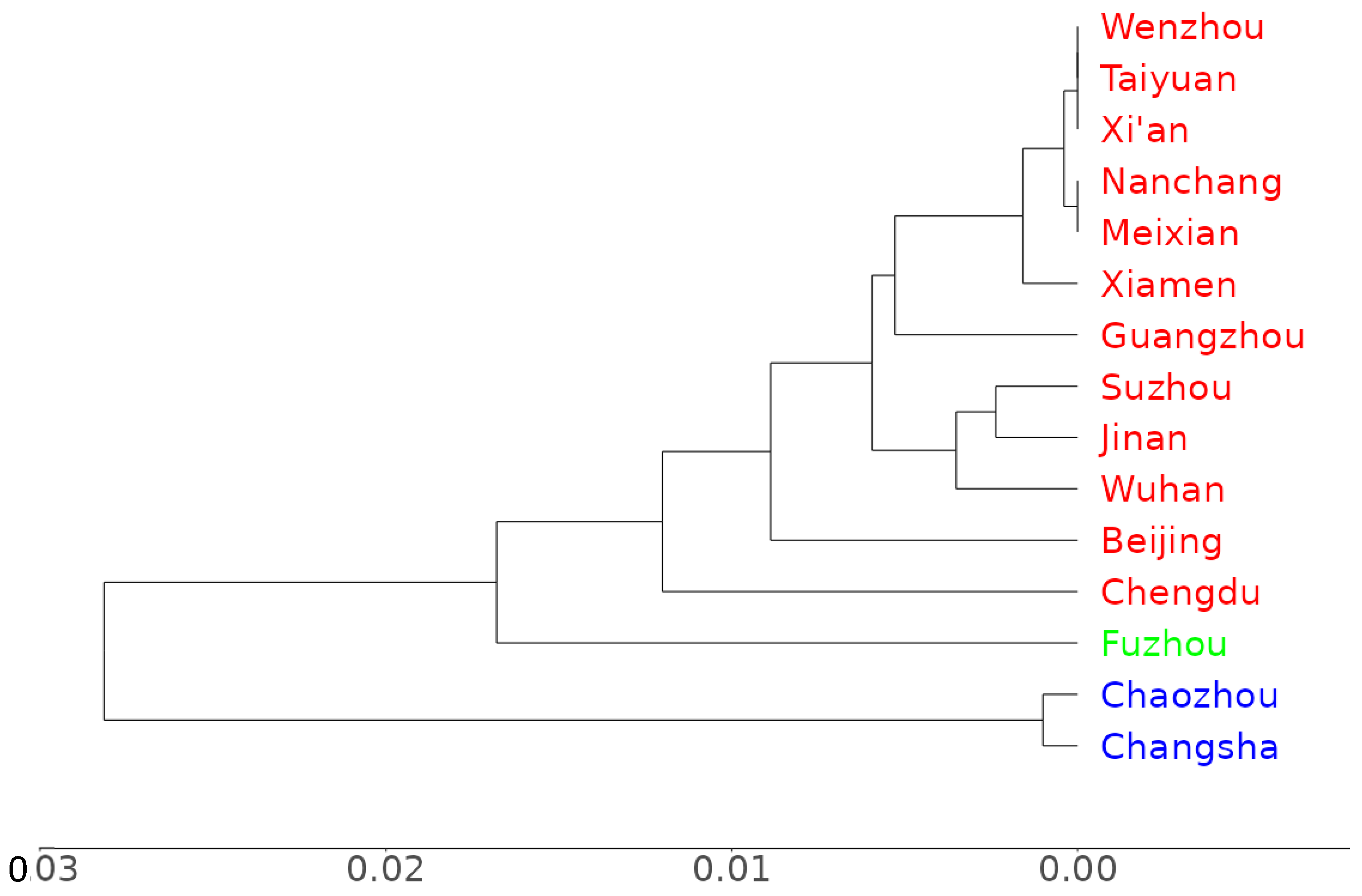
2.3.1. Cluster Analysis
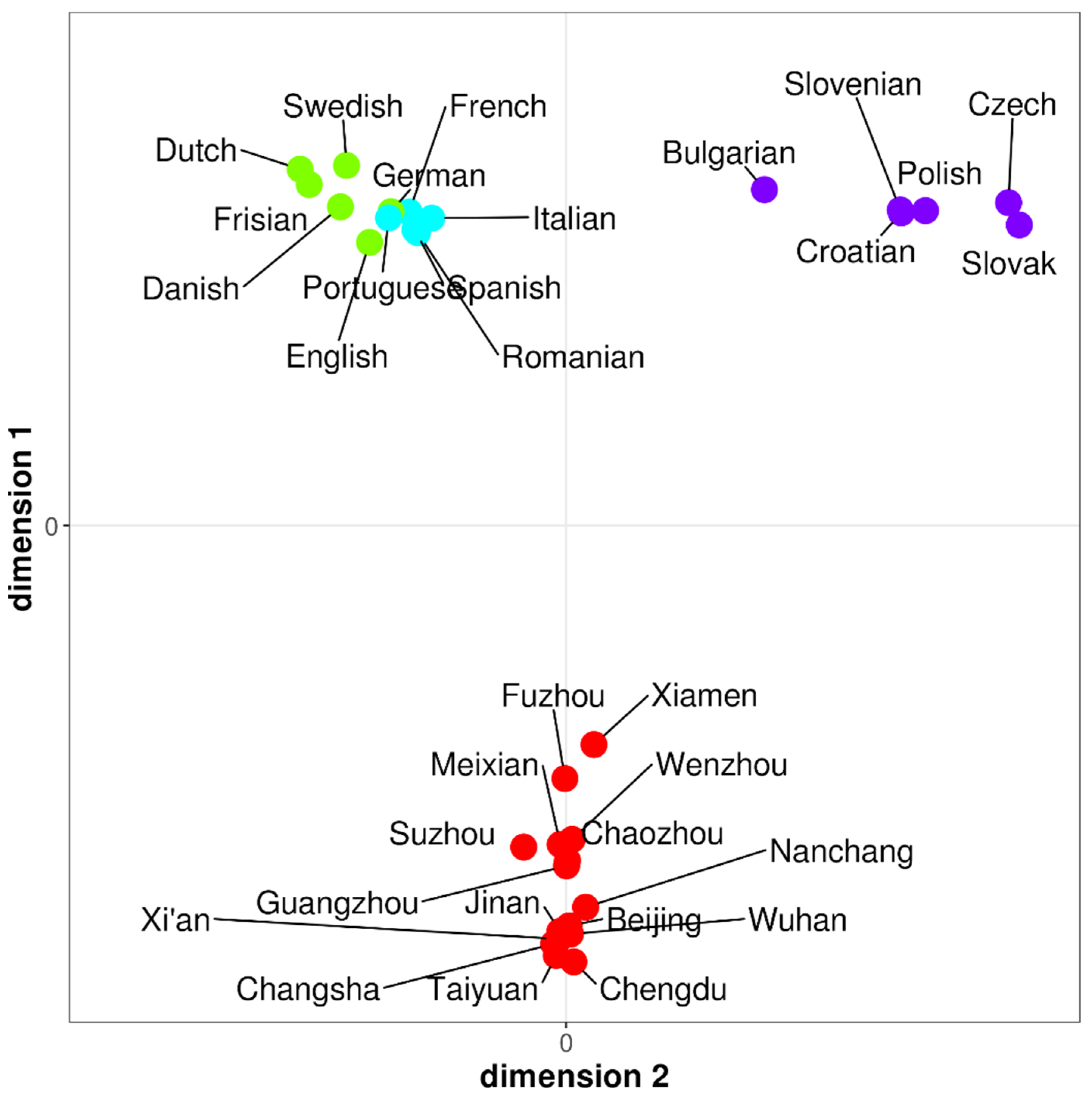
2.3.2. Multi-Dimensional Scaling
3. Results
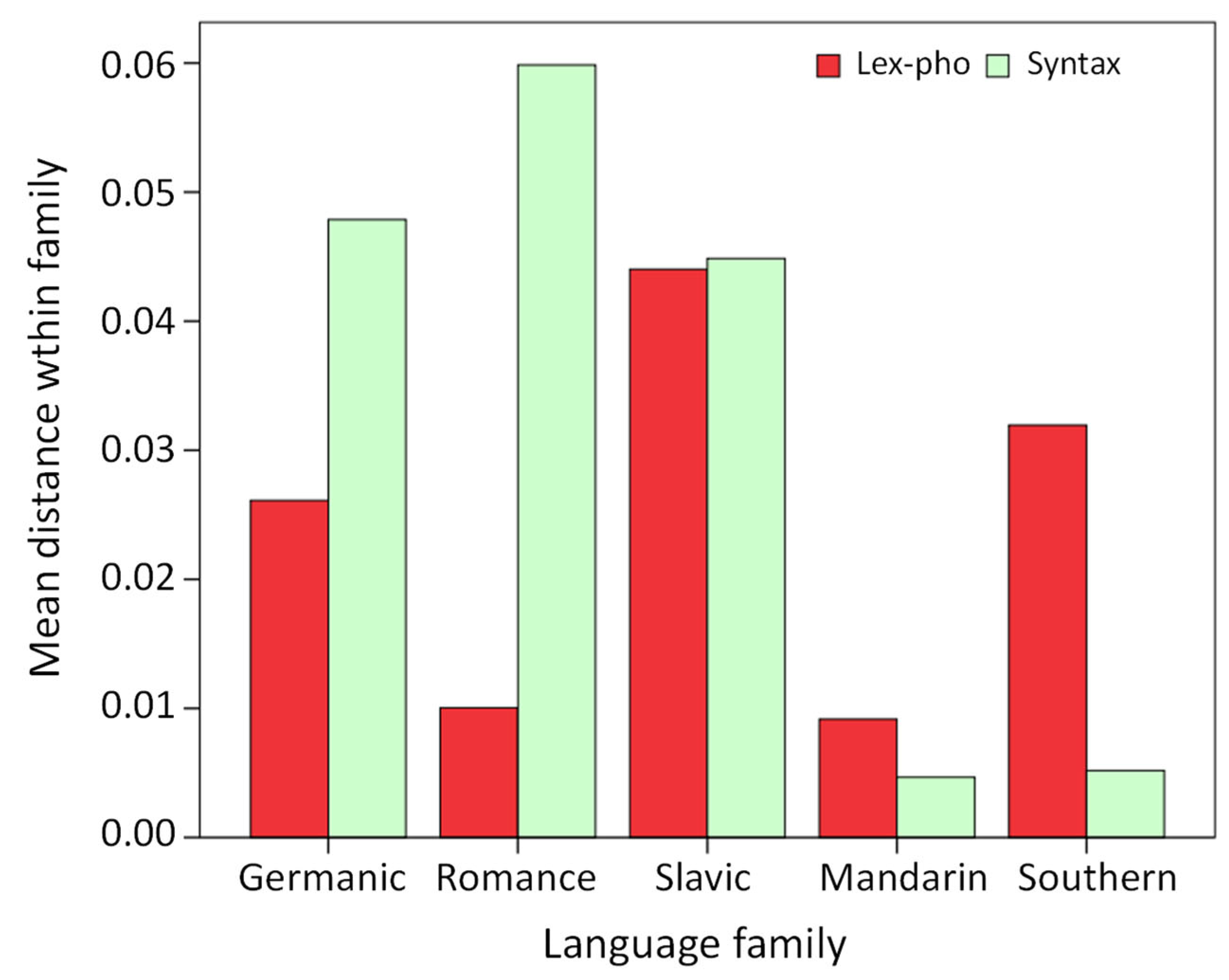
3.1. Lexico-Phonetic Measurements
3.2. Syntactic Measurements
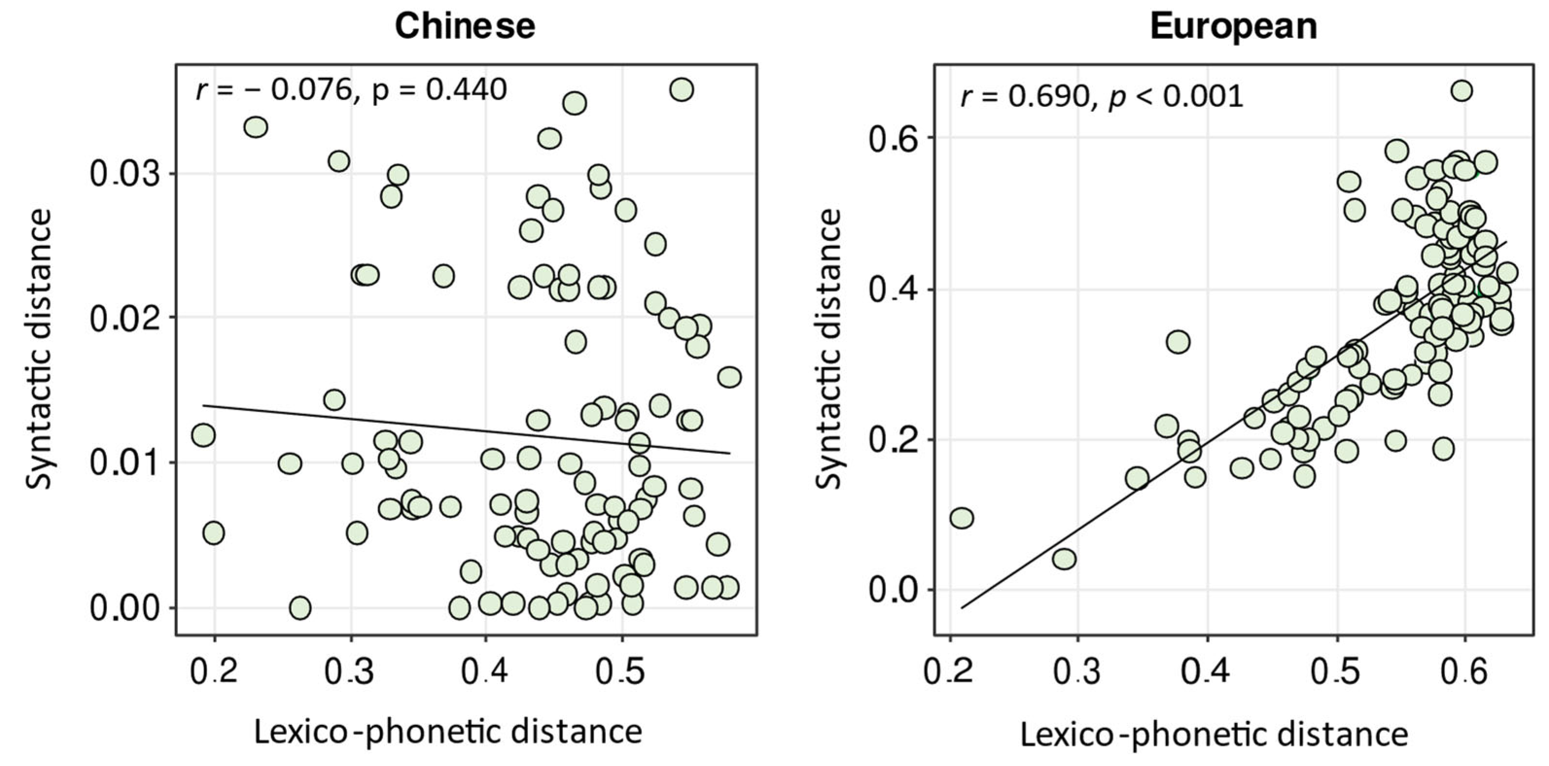
3.3. Correlating the Domains
4. Comparison and Discussion
4.1. Comparison with Published Affinity Trees
4.2. PoS Trigram Frequencies and Word Order Typology
4.3. Separating Lexical and Phonetic Distance by Automatic Cognate Recognition
5. Conclusions
Author Contributions
Funding
Informed Consent Statement
Data Availability Statement
Conflicts of Interest
Appendix A. The 100 Most Frequent Nouns in the BNC Corpus and Their Equivalents in Mandarin Chinese10
| English | Chinese | English | Chinese | English | Chinese | English | Chinese |
| time | 时间 | place | 地方 | development | 发展 | hour | 小时 |
| year | 年 | point | 点 | room | 房间 | rate | 比率 |
| people | 人 (们) | house | 房子 | water | 水 | law | 法律 |
| man | 男 (人) | country | 国家 | form | 表格 | door | 门 |
| day | (一) 天 | week | 周 | car | 汽车 | court | 法庭 |
| thing | 事情 | member | 会员 | level | 水平 | office | 办公室 |
| child | 孩子 | end | 尽头 | policy | 政策 | war | 战争 |
| government | 政府 | word | 单词 | council | 理事会 | reason | 原因 |
| part | 部分 (零件) | example | 例子 | line | 线 (条) | minister | 部长 |
| life | 生活 | family | 家 | need | 需要 | subject | 主题 |
| case | 情况 | fact | 事实 | effect | 效果 | person | 人 |
| woman | 女人 | percent | 百分比 | use | 使用 | period | 期间 |
| work | 工作 | month | 月 (份) | idea | 主意 | society | 社会 |
| system | 系统 | side | (旁) 边 | study | 研究 | process | 过程 |
| group | 组 | night | 夜晚 | girl | 女孩 | mother | 母亲 |
| number | 数字 | eye | 眼睛 | name | 名字 | voice | 声音 |
| world | 世界 | head | 头 | result | 结果 | police | 警察 |
| area | 区域 | information | 信息 | body | 身体 | kind | 种类 |
| course | 课程 | question | 问题 | friend | 朋友 | price | 价格 |
| company | 公司 | power | 权力 | right | 权利 | position | 位置 |
| problem | 问题 | money | (金) 钱 | authority | 权威 | age | 年龄 |
| service | 服务 | change | 变化 | view | 视野 | figure | 体型 |
| hand | 手 | interest | 兴趣 | report | 报告 | education | 教育 |
| party | 派对 | order | 订单 | face | 脸 | programme | 日程 |
| school | 学校 | book | 书 | market | 市场 | minute | 分钟 |
Appendix B. The Four Short Texts in English and in Mandarin That Were Used to Compute PoS Trigram Frequencies for 32 Language Varieties11
Parents whose children show a special interest in a particular sport have a difficult decision to make. Should they allow their children to train to become top sportsmen and women? For many children it means starting very young. School work, going out with friends and other interests have to take second place. It’s very difficult to explain to young children why they have to train for five hours a day. That includes even the weekend, when most of their friends are playing. Another problem is of course money. In many countries money for training is available from the government for the very best young athletes. If this help cannot be given the parents have to find the time and money to support their children. Sports clothes, transport to competitions, special equipment etc. can all be very expensive. Many parents are understandably worried that it’s dangerous to start serious training in a sport at an early age. Some doctors agree that young muscles may be damaged by training before they are properly developed. Trainers, however, believe that you can only reach the top as a sports person when you start young. What is clear is that very few people do reach the top. So both parents and children should be prepared for failure. It happens even after many years of training.
对于 那些 孩子 对 某项 特定 运动 表现 出 特别 兴趣 的 父母 来说,他们 需要 做出 一个 艰难 的 决定 。他们 是否 应该 允许 孩子 接受 训练, 成为 顶级 运动员? 对于 许多 孩子 来说, 这 意味 着 从 很 小 的 时候 就 开始 学业、 与 朋友 出去 玩 和 其他 兴趣 都 必须 放 在 第二位。很 难 向 年幼 的 孩子 解释 为什么 他们 每天 要 训练 五个 小时, 甚至 包括 周末, 这 时候 他们 的 大部分 朋友 都 在 玩耍。另一 个 问题 当然 是 金钱。在 许多 国家, 政府 为 最 优秀 的 年轻 运动员 提供 训练 资金。如果 得不到 这种 资助, 父母 就 必须 找到 时间 和 金钱 来 支持 孩子。运动 服装、 比赛 的 交通费、 特殊 装备 等 都 可能 非常 昂贵。许多 父母 担心 在 孩子 年幼 时 进行 严格 的 运动 训练 可能 会 对 肌肉 造成 损伤。一些 医生 同意, 在 肌肉 适当 发育 之前 进行 训练 可能 会 对 年幼 的 肌肉 造成 损害。然而, 教练们 相信, 只有 在 年幼 时 训练 才能 成为 顶级 运动员。显而易见 的 是, 很少 有人 能 达到 顶峰。 因此, 父母 和 孩子 都 应该 为 失败 做 好 准备。即使 经过 多年 的 训练, 失败 也 是 有 可能 发生 的。
Hello, my name is Bill and I give advice to people with questions about their health. I get a lot of letters at this time of year. People complain that they have a cold which won’t go away. There are so many different stories about how to prevent or cure a cold. So it’s often difficult to know what to do. Colds are rarely dangerous, except for people who are already weak, such as the elderly or young babies. Still, colds are always uncomfortable and usually most unpleasant. Of course you can buy lots of medicines which will help to make your cold less unpleasant. But remember that nothing can actually cure a cold or make it go away faster. Another thing is that any medicine which is strong enough to make you feel better could be dangerous. If you are already taking medicine for other illnesses always check with your doctor if that’s all right. And remember that it could happen that they might make you sleepy. Please don’t try to drive if they do! Lastly, there are no magic foods or drinks. The best answer is to keep strong and healthy. You’ll have less chance of catching a cold, and if you do, it shouldn’t be so bad!
你好, 我的 名字 叫 克里斯蒂娜, 我 为 有 健康 疑问 的 人 提供 建议。每年 此 时, 我 都 会 收到 许多 来信。人们 抱怨 他们 的 感冒 不 消退。关于 预防 或 治疗 感冒, 有 很多 不同 的 说法, 所以 往往 很 难 知道 该 怎么 做。感冒 很少 有 危险, 除非 对 本就 虚弱 的 人,如 老人 或 婴儿。 然而, 感冒 总是 让 人 不 舒服, 而且 通常 也 很 不 愉快。当然, 你 可以 买 很多 药, 这 将 有助于 减轻 感冒 的 不适感。但是 请 记住, 没有 药物 能 真正 治愈 感冒, 或者 让 它 好 得 更 快。另外, 任何 能 让 你 感觉 好些 的 药物 都 可能 是 危险的。如果 你 已经 在 服用 治疗 其他 疾病 的 药物, 请 务必 咨询 你 的 医生, 与 感冒药 一同 服用 是否 可以。而且 请 记住, 药物 可能 会 让 你 昏昏欲睡。如果 出现 这种 情况, 请 不要 尝试 开车! 最后, 没有 什么 神奇 的 食物 或 饮料。最好 的 办法 就是 保持 强壮 和 健康。 这样 你 感冒 的 机会 会 更 小, 即使 感冒 了, 也 不会 那么 糟糕!
Winter is dangerous because it’s so difficult to know what is going to happen. Accidents take place so easily. Fog can be waiting to meet you over the top of a hill. Ice might be hiding beneath the melting snow, waiting to send you off the road. The car coming towards you may suddenly slide across the road. Rule Number One for driving on icy roads is to drive smoothly. Uneven movements can make a car suddenly very difficult to control. Every time you turn the wheel, brake or increase speed, you must be gentle and slow as possible. Imagine you are driving with a full cup of hot coffee on the seat next to you. Drive so that you wouldn’t spill it. Rule Number Two is to pay attention to what might happen. The more ice there is, the further down the road you have to look. Test how long it takes to stop by gently braking. Remember that you may be driving more quickly than you think. In general, allow double your normal stopping distance when the road is wet. Use three times this distance on snow, and even more on ice. Try to stay in control of your car at all times and you will avoid trouble.
冬季 (驾驶) 很 危险, 因为 很 难 知道 会 发生 什么 事情。 事故 很 容易 发生。 雾 可能 在 山顶 等 着 见 你。冰 可能 隐藏 在 融化 的 雪 下, 等 着 把 你 甩 出 路面。向 你 驶 来 的 车 可能 会 突然 滑 过 道路。在 冰雪 路面 驾驶 的 第一 规则 是 平稳 驾驶。不 平稳 的 动作 会 使 车辆 突然 难以 控制。每次 你 转动 方向盘、 刹车 或 加速 时, 都 要 尽量 轻柔 和 缓慢。想象 一下, 你 正在 开车,满满 一杯 热 咖啡 放 在 旁边 的 座位 上。平稳 地 驾驶, 确保 你 别 撒 了 咖啡。第二 规则 是 要 注意 可能 发生 的 情况。冰面 越 多, 你 就 越 需要 更 远 地 向前 看。 通过 轻轻 刹车 来 测试 停车 需要 多长 时间。记住, 你 驾驶 的 速度 可能 比 你 想象 的 要 快。一般来说, 当 路面 湿滑 时, 允许 你 的 停车 距离 是 平时 的 两倍。在 雪地 上 则要 增加 三倍 的 停车 距离, 在 冰面 上 要 更 多 (距离)。尽量 一直 控制 好 你 的 车, 这样 你 就 能 避免 麻烦。
Getting enough exercise is part of a healthy lifestyle. Along with jogging and swimming, riding a bike is one of the best all-round forms of exercise. It can help to increase your strength and energy. Also it gives you more efficient muscles and a stronger heart. But increasing your strength is not the only advantage of riding a bike. You’re not carrying the weight of your body on your feet. That’s why riding a bike is a good form of exercise for people with painful feet or backs. However, with all forms of exercise it’s important to start slowly and build up gently. Doing too much too quickly can damage muscles that aren’t used to working. If you have any doubts about taking up riding a bike for health reasons, talk to your doctor. Ideally you should be riding a bike at least two or three times a week. For the exercise to be doing you good, you should get a little out of breath. Don’t worry that if you begin to lose your breath, it could be dangerous. This is simply not true. Shortness of breath shows that the exercise is having the right effect. However, if you find you are in pain then you should stop and take a rest. After a while it will get easier.
保持 充足 的 运动 是 健康 生活 方式 的 一 部分。 除了 慢跑 和 游泳, 骑 自行车 也 是 最好 的 全方位 锻炼 方式 之一。它 可以 帮助 增加 你 的 力量 和 能量, 使 你 的 肌肉 更加 高效, 心脏 更 强壮。但 增加 力量 并 不是 骑 自行车 的 唯一 好处。 你 的 脚 没有 承受 你 身体 的 重量。这 就是 为什么 骑 自行车 对于 脚痛 或 背痛 的 人 来说 是 一种 很好 的 锻炼 方式。然而, 对于 所有 形式 的 锻炼 来说, 缓慢 开始、 逐渐 增加 是 很 重要的。过快 过多 的 运动 可能 会 损伤 不习惯 工作 的 肌肉。 如果 你 因 健康 原因 对 骑 自行车 有 任何 疑虑, 请 咨询 医生。理想 情况 下, 你 应该 每周 至少 骑 自行车 两 到 三次。为了 使 锻炼 对 你 有益, 你 应该 稍微 有些 气喘。 不要 担心 如果 你 开始 喘 不过 气, 这 可能 是 危险的。这 完全 不是 真的。呼吸 急促 表明 锻炼 产生 了 正确 的 效果。然而, 如果 你 发现 自己 感到 疼痛, 那 就 应该 停 下来 休息 一下。过 一段 时间 后, 情况 会 变 得 更 容易。
Appendix C
| Bu | Cr | Cz | Da | Du | En | Fh | Fn | Ge | It | Po | Pt | Ro | Sk | Sn | Sp | Sw | |
| Bu | 0.377 | 0.515 | 0.592 | 0.563 | 0.588 | 0.597 | 0.577 | 0.594 | 0.548 | 0.512 | 0.510 | 0.514 | 0.509 | 0.475 | 0.547 | 0.591 | |
| Cr | 0.330 | 0.464 | 0.616 | 0.584 | 0.632 | 0.613 | 0.587 | 0.580 | 0.561 | 0.490 | 0.586 | 0.554 | 0.470 | 0.368 | 0.551 | 0.605 | |
| Cz | 0.317 | 0.217 | 0.627 | 0.605 | 0.614 | 0.603 | 0.598 | 0.591 | 0.576 | 0.385 | 0.614 | 0.591 | 0.209 | 0.451 | 0.603 | 0.595 | |
| Da | 0.417 | 0.396 | 0.378 | 0.512 | 0.583 | 0.605 | 0.526 | 0.518 | 0.602 | 0.628 | 0.594 | 0.577 | 0.628 | 0.614 | 0.588 | 0.475 | |
| Du | 0.547 | 0.482 | 0.458 | 0.257 | 0.543 | 0.570 | 0.289 | 0.427 | 0.554 | 0.602 | 0.572 | 0.538 | 0.609 | 0.583 | 0.580 | 0.471 | |
| En | 0.440 | 0.422 | 0.389 | 0.188 | 0.269 | 0.580 | 0.546 | 0.570 | 0.569 | 0.613 | 0.558 | 0.545 | 0.626 | 0.618 | 0.580 | 0.546 | |
| Fh | 0.664 | 0.567 | 0.558 | 0.338 | 0.354 | 0.261 | 0.571 | 0.610 | 0.490 | 0.591 | 0.471 | 0.508 | 0.600 | 0.616 | 0.508 | 0.581 | |
| Fn | 0.558 | 0.491 | 0.465 | 0.275 | 0.042 | 0.274 | 0.363 | 0.474 | 0.560 | 0.601 | 0.579 | 0.541 | 0.616 | 0.588 | 0.582 | 0.478 | |
| Ge | 0.569 | 0.489 | 0.456 | 0.295 | 0.162 | 0.302 | 0.376 | 0.185 | 0.580 | 0.588 | 0.601 | 0.555 | 0.589 | 0.594 | 0.599 | 0.484 | |
| It | 0.587 | 0.496 | 0.487 | 0.377 | 0.381 | 0.314 | 0.213 | 0.372 | 0.405 | 0.570 | 0.449 | 0.436 | 0.588 | 0.581 | 0.345 | 0.566 | |
| Po | 0.314 | 0.215 | 0.198 | 0.354 | 0.449 | 0.393 | 0.563 | 0.468 | 0.446 | 0.483 | 0.604 | 0.581 | 0.386 | 0.502 | 0.605 | 0.593 | |
| Pt | 0.543 | 0.454 | 0.431 | 0.331 | 0.366 | 0.286 | 0.229 | 0.368 | 0.396 | 0.174 | 0.445 | 0.479 | 0.616 | 0.602 | 0.390 | 0.577 | |
| Ro | 0.504 | 0.396 | 0.391 | 0.314 | 0.380 | 0.279 | 0.252 | 0.384 | 0.404 | 0.228 | 0.370 | 0.199 | 0.602 | 0.575 | 0.458 | 0.569 | |
| Sk | 0.309 | 0.202 | 0.095 | 0.359 | 0.455 | 0.395 | 0.557 | 0.464 | 0.469 | 0.487 | 0.185 | 0.443 | 0.383 | 0.463 | 0.608 | 0.603 | |
| Sn | 0.286 | 0.217 | 0.252 | 0.376 | 0.480 | 0.403 | 0.569 | 0.502 | 0.469 | 0.530 | 0.232 | 0.483 | 0.444 | 0.261 | 0.578 | 0.598 | |
| Sp | 0.584 | 0.505 | 0.501 | 0.347 | 0.377 | 0.291 | 0.185 | 0.372 | 0.404 | 0.148 | 0.497 | 0.151 | 0.209 | 0.494 | 0.520 | 0.582 | |
| Sw | 0.406 | 0.367 | 0.359 | 0.152 | 0.277 | 0.198 | 0.339 | 0.296 | 0.310 | 0.349 | 0.333 | 0.337 | 0.315 | 0.356 | 0.366 | 0.348 | |
| Bu: Bulgarian, Cr: Croatian, Cz: Czech, Da: Danish, Du: Dutch, En: English, Fh: French, Fn: Frisian, Ge: German, It: Italian: Po: Polish, Pt: Portuguese: Ro: Romanian, Sk: Slovak, Sn: Slovenian, Sp: Spanish, Sw: Swedish. | |||||||||||||||||
Appendix D
| Be | Cs | Cz | Cd | Fu | Gu | Ji | Me | Na | Su | Ta | We | Wu | X’n | Xm | |
| Beijing | 0.335 | 0.485 | 0.288 | 0.558 | 0.473 | 0.333 | 0.482 | 0.411 | 0.513 | 0.346 | 0.514 | 0.344 | 0.329 | 0.551 | |
| Changsha | 0.032 | 0.459 | 0.230 | 0.544 | 0.438 | 0.330 | 0.443 | 0.369 | 0.433 | 0.309 | 0.461 | 0.291 | 0.312 | 0.548 | |
| Chaozhou | 0.031 | 0.001 | 0.447 | 0.465 | 0.449 | 0.503 | 0.454 | 0.461 | 0.525 | 0.425 | 0.487 | 0.483 | 0.483 | 0.466 | |
| Chengdu | 0.015 | 0.036 | 0.035 | 0.525 | 0.432 | 0.326 | 0.405 | 0.328 | 0.438 | 0.255 | 0.462 | 0.191 | 0.301 | 0.513 | |
| Fuzhou | 0.021 | 0.038 | 0.037 | 0.023 | 0.487 | 0.556 | 0.478 | 0.505 | 0.580 | 0.503 | 0.549 | 0.535 | 0.552 | 0.528 | |
| Guangzhou | 0.009 | 0.030 | 0.029 | 0.011 | 0.015 | 0.499 | 0.424 | 0.414 | 0.518 | 0.457 | 0.478 | 0.430 | 0.487 | 0.505 | |
| Jinan | 0.010 | 0.031 | 0.030 | 0.012 | 0.019 | 0.007 | 0.496 | 0.431 | 0.502 | 0.305 | 0.480 | 0.389 | 0.199 | 0.554 | |
| Meixian | 0.008 | 0.025 | 0.024 | 0.011 | 0.014 | 0.005 | 0.005 | 0.380 | 0.514 | 0.453 | 0.508 | 0.430 | 0.485 | 0.482 | |
| Nanchang | 0.008 | 0.025 | 0.024 | 0.011 | 0.014 | 0.005 | 0.005 | 0.000 | 0.468 | 0.403 | 0.477 | 0.345 | 0.420 | 0.507 | |
| Suzhou | 0.011 | 0.028 | 0.027 | 0.014 | 0.017 | 0.008 | 0.002 | 0.004 | 0.004 | 0.448 | 0.459 | 0.438 | 0.517 | 0.571 | |
| Taiyuan | 0.007 | 0.025 | 0.024 | 0.011 | 0.014 | 0.005 | 0.006 | 0.000 | 0.000 | 0.003 | 0.439 | 0.351 | 0.263 | 0.548 | |
| Wenzhou | 0.007 | 0.025 | 0.024 | 0.011 | 0.014 | 0.005 | 0.006 | 0.000 | 0.000 | 0.003 | 0.000 | 0.495 | 0.474 | 0.578 | |
| Wuhan | 0.012 | 0.033 | 0.032 | 0.013 | 0.021 | 0.007 | 0.003 | 0.008 | 0.008 | 0.004 | 0.008 | 0.008 | 0.374 | 0.524 | |
| Xi’an | 0.007 | 0.025 | 0.024 | 0.011 | 0.014 | 0.005 | 0.006 | 0.000 | 0.000 | 0.003 | 0.000 | 0.000 | 0.008 | 0.567 | |
| Xiamen | 0.009 | 0.021 | 0.020 | 0.012 | 0.015 | 0.006 | 0.007 | 0.002 | 0.002 | 0.005 | 0.002 | 0.002 | 0.009 | 0.002 |
Appendix E
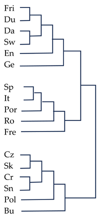 |  |
| Polyakov et al. (2009) | Present study |
Appendix F
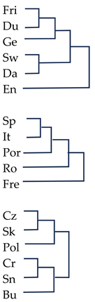
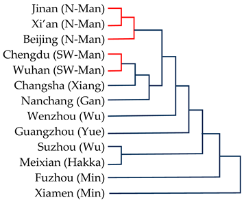 | 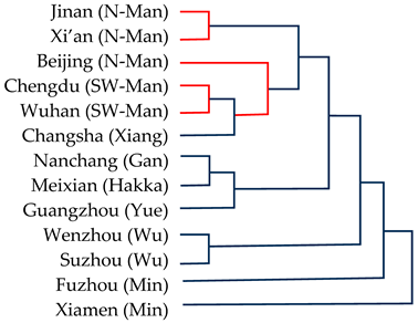 | ||
| Müller et al. (2021) | Present study | ||
| 1 | Appendix E and Appendix F contain a comparison of the affinity trees produced on the basis of the ASJP database and ours. The lexico-phonetic distances computed by both methods for the 32 language varieties at issue correlate at r = 0.925. See also Section 4. |
| 2 | This claim may not be true in the case of onomatopoeic words and word forms based on sound symbolism. As a precaution, Wichmann et al. (2010) therefore propose that the mean length-normalized Levenstein distance (LDN) computed on all cognate pairs be divided by the mean LDN for all non-cognate pairs. This ratio (LDND) was found to be a slightly (but not significantly) better predictor of cladistic language trees than LDN. |
| 3 | West Frisian is a West Germanic language spoken as the native language by an estimated 415,000 citizens in the north of the Netherlands (Robinson-Jones & Scarse, 2022, p. 3). It has an official status along with and equal to Dutch in the province of Friesland/Fryslân. The language was included in the present study by special request of the Frisian Academy. |
| 4 | We used LED-A for calculating the PMI Levenshtein distances. The implementation of PMI–Levenshtein in LED-A differs in its details from Wieling (2012). See https://www.led-a.org/docs/PMI.pdf (accessed on 21 May 2025). |
| 5 | See also: https://www.led-a.org/docs/Diacr.pdf (accessed on 21 May 2025). |
| 6 | See also: https://www.led-a.org/docs/Ngram.pdf (accessed on 21 May 2025). |
| 7 | This result mirrors earlier findings by Gooskens and Heeringa (2004), computed on phonetically transcribed readings of the Aesop North wind and sun fable, which clearly showed that, contrary to popular belief, Frisian is (much) closer to Dutch than to English—or any other Germanic language. It is true, nevertheless, that the distance between English and Frisian is (slightly) smaller than between English and Dutch—both in our and earlier results. The urban legend is perpetuated by selective sampling of the striking similarities between English and Frisian, such as those mentioned by Pei (1966, p. 34). |
| 8 | We also checked this using the Mantel test and obtained the same findings. |
| 9 | See https://lingpy.org/ (accessed on 21 May 2025). |
| 10 | The parallel lists of the orthographic form, IPA transcription and (for Chinese) Romanized Pinyin (including lexical tone) of the 100 items for each of the 32 language varieties can be downloaded from the OSF site (see section “Data Availability Statement”). |
| 11 | The complete texts with PoS tags added after each word can be downloaded from the OSF site (see section “Data Availability Statement”). |
References
- BNC Consortium. (2007). BNC: The British National Corpus, version 3, BNC XML edition. Oxford University Computing Services on Behalf of the BNC Consortium. Available online: http://www.natcorp.ox.ac.uk/ (accessed on 21 May 2025).
- Bruce, G. (1977). Swedish word accents in sentence perspective. Liber. Available online: https://portal.research.lu.se/en/publications/311242e6-5f2b-489a-b35d-5ffef5ec5301 (accessed on 21 May 2025).
- Ceolin, A., Guardiano, C., Irimia, M. A., & Longobardi, G. (2020). Formal syntax and deep history. Frontiers in Psychology, 11, 488871. [Google Scholar] [CrossRef] [PubMed]
- Ceolin, A., Guardiano, C., Longobardi, G., Irimia, M. A., Bortolussi, L., & Sgarro, A. (2021). At the boundaries of syntactic prehistory. Philosophical Transactions of the Royal Society, 376, 20200197. [Google Scholar] [CrossRef] [PubMed]
- Cheng, C.-C. (1997). Measuring relationship among dialects: DOC and related resources. Computational Linguistics & Chinese Language Processing, 2(1), 41–72. Available online: https://aclanthology.org/O97-3002/ (accessed on 21 May 2025).
- Council of Europe. (2001). Common European framework of reference for languages. Learning, teaching, assessment. Cambridge University Press. Available online: https://rm.coe.int/1680459f97 (accessed on 21 May 2025).
- Di Buccio, E., Di Nunzio, G. M., & Silvello, G. (2014). A vector space model for syntactic distances between dialects. In Language resources and evaluation conference (pp. 2486–2489). ELRA. Available online: https://aclanthology.org/L14-1148/ (accessed on 21 May 2025).
- Dryer, M. S., & Haspelmath, M. (Eds.). (2013). WALS online (v2020.4) [data set]. Zenodo. Available online: https://wals.info (accessed on 21 May 2025). [CrossRef]
- Dunn, M., Greenhill, S. J., Levinson, S. C., & Gray, R. D. (2011). Evolved structure of language shows lineage-specific trends in word-order universals. Nature, 473, 79–82. [Google Scholar] [CrossRef]
- Dunn, M., Terrill, A., Reesink, G., Foley, R. A., & Levinson, S. C. (2005). Structural phylogenetics and the reconstruction of ancient language history. Science, 309, 2072–2075. [Google Scholar] [CrossRef]
- Dyen, I., Kruskal, J. B., & Black, P. (1992). An Indoeuropean classification: A lexicostatistical experiment (Transactions of the American Philosophical Society 82.5). University of Pennsylvania Press. Available online: http://www.ldc.upenn.edu/ (accessed on 21 May 2025). [CrossRef]
- Gårding, E. (1974). Kontrastiv prosodi. Gleerup. [Google Scholar]
- Golubović, J. (2016). Mutual intelligibility in the Slavic language area. Center for Language and Cognition. Available online: https://research.rug.nl/files/31880596/Complete_thesis.pdf (accessed on 21 May 2025).
- Gooskens, C. (2024). Mutual intelligibility between closely related languages. De Gruyter Mouton. [Google Scholar] [CrossRef]
- Gooskens, C., & Heeringa, W. (2004). The position of Frisian in the Germanic language area. In D. G. Gilbers, M. J. Schreuder, & N. Knevel (Eds.), On the boundaries of phonology and phonetics (pp. 61–87). Department of Linguistics, Groningen University. Available online: https://www.researchgate.net/publication/237534065 (accessed on 21 May 2025).
- Gooskens, C., & van Heuven, V. J. (2017). Measuring cross-linguistic intelligibility in the Germanic, Romance and Slavic language groups. Speech Communication, 89, 25–36. [Google Scholar] [CrossRef]
- Gooskens, C., & van Heuven, V. J. (2020). How well can intelligibility of closely related languages in Europe be predicted by linguistic and non-linguistic variables? Linguistic Approaches to Bilingualism, 10(3), 351–379. [Google Scholar] [CrossRef]
- Gooskens, C., & van Heuven, V. J. (2021). Mutual intelligibility. In M. Zampieri, & P. Nakov (Eds.), Similar languages, varieties, and dialects: A computational perspective (pp. 51–95). Cambridge University Press. [Google Scholar] [CrossRef]
- Gooskens, C., van Heuven, V. J., Golubović, J., Schüppert, A., Swarte, F., & Voigt, S. (2018). Mutual intelligibility between closely related languages in Europe. International Journal of Multilingualism, 15(2), 169–193. [Google Scholar] [CrossRef]
- Gray, R. D., & Atkinson, Q. D. (2003). Language-tree divergence times support the Anatolian theory of Indo-European origin. Nature, 426, 435–439. [Google Scholar] [CrossRef]
- Gray, R. D., Bryant, D., & Greenhill, S. (2010). On the shape and fabric of human history. Philosophical Transactions of the Royal Society, 365, 3923–3933. [Google Scholar] [CrossRef]
- Heeringa, W. (2004). Measuring dialect pronunciation differences using Levenshtein distance (Groningen Dissertations in Linguistics 46). Groningen Centre for Language and Cognition. Available online: https://research.rug.nl/files/9800656/thesis.pdf (accessed on 21 May 2025).
- Heeringa, W., Gooskens, C., & van Heuven, V. J. (2023). Comparing Germanic, Romance and Slavic: Relationships among linguistic distances. Lingua, 287, 1–23. [Google Scholar] [CrossRef]
- Heeringa, W., Swarte, F., Schüppert, A., & Gooskens, C. (2018). Measuring syntactical variation in Germanic texts. Digital Scholarship in the Humanities, 33(1), 279–296. [Google Scholar] [CrossRef]
- Inkelas, S., & Zec, D. (1988). Serbo-croatian pitch accent: The interaction of tone, stress and intonation. Language, 64(2), 227–248. [Google Scholar] [CrossRef]
- Jain, A. K., & Dubes, R. C. (1988). Algorithms for clustering data. Prentice Hall. [Google Scholar]
- Jäger, G. (2013). Phylogenetic inference from word lists using weighted alignment with empirically determined weights. Language Dynamics and Change, 3(2), 245–291. [Google Scholar] [CrossRef]
- Kessler, B. (1995, March 27–31). Computational dialectology in Irish Gaelic. 7th Conference of the European Chapter of the Association for Computational Linguistics (pp. 60–67), Dublin, Ireland. Available online: https://aclanthology.org/E95-1009/ (accessed on 21 May 2025).
- Li, C., & Thompson, S. (1981). Mandarin Chinese: A functional reference grammar. University of California Press. [Google Scholar]
- Li, R. (Ed.). (1993–1999). The comprehensive dictionaries of modern Chinese dialects. Jiang Su Education Publishing House. [Google Scholar]
- List, J.-M. (2012, April 23–24). LexStat: Automatic detection of cognates in multilingual wordlists. EACL 2012 Joint Workshop of LINGVIS & UNCLH (pp. 117–125), Avignon, France. Available online: https://aclanthology.org/W12-0216.pdf (accessed on 21 May 2025).
- List, J.-M. (2014). Sequence comparison in historical linguistics. Düsseldorf University Press. [Google Scholar] [CrossRef]
- Longobardi, G. (2005). A minimalist program for parametric linguistics. In H. Broekhuis, N. Corver, R. Huijbregts, U. Kleinhenz, & J. Koster (Eds.), Organizing grammar (pp. 407–414). DeGruyter Mouton. Available online: https://people.sissa.it/~ale/EU_infoday/Lon05.pdf (accessed on 21 May 2025).
- Mian Yan, M. (2006). Introduction to Chinese dialectology (LINCOM Studies in Asian Linguistics). LINCOM. Available online: https://starlingdb.org/Texts/Students/Mian%20Yan%2C%20Margaret/Introduction%20to%20Chinese%20Dialectology%20%282006%29.pdf (accessed on 21 May 2025).
- Mongeau, M., & Sankoff, D. (1990). Comparison of musical sequences. Computers and the Humanities, 24(3), 161–175. [Google Scholar] [CrossRef]
- Müller, A., Velupillai, V., Wichmann, S., Brown, C. H., Holman, E. W., Sauppe, S., Brown, P., Hammarström, H., Belyaev, O., List, J.-M., Bakker, D., Egorov, D., Urban, M., Mailhammer, R., Dryer, M. S., Korovina, E., Beck, D., Geyer, H., Epps, P., … Valenzuela, P. (2021). ASJP world language trees of lexical similarity: Version 5 (October 2021). Available online: https://asjp.clld.org/static/WorldLanguageTree-005.zip (accessed on 21 May 2025).
- Nerbonne, J., & Wiersma, W. (2006). A measure of aggregate syntactic distance. In J. Nerbonne, & E. Hinrichs (Eds.), Proceedings of the workshop on linguistic distances (pp. 82–90). Association for Computational Linguistics. Available online: https://aclanthology.org/W06-1111.pdf (accessed on 21 May 2025).
- Pei, M. (1966). The story of language. Allen & Unwin. [Google Scholar]
- Polyakov, V. N., Solovyev, V. D., Wichmann, S., & Belyaev, O. (2009). Using WALS and Jazyki Mira. Linguistic Typology, 13, 135–165. [Google Scholar] [CrossRef]
- Pompei, S., Loreto, V., & Tria, F. (2011). On the accuracy of language trees. PLoS ONE, 6(6), e20109. [Google Scholar] [CrossRef]
- Riad, T. (2014). The phonology of Swedish. Oxford University Press. [Google Scholar]
- Robinson-Jones, C., & Scarse, Y. R. (2022). Report on the West Frisian language (Language technology support of Europe’s languages in 2020/2021—European language equality project). Available online: https://www.researchgate.net/publication/361644854 (accessed on 21 May 2025).
- Séguy, J. (1973). La dialectometrie dans l’Atlas linguistique de la Gascogne. Revue de Linguistique Romane, 37, 1–24. [Google Scholar]
- Sokal, R. R., & Rohlf, F. J. (1962). The comparison of dendrograms by objective methods. Taxon, 11, 33–40. [Google Scholar] [CrossRef]
- Swadesh, M. (1952). Lexico-statistic dating of prehistoric ethnic contacts: With special reference to North American Indians and Eskimos. Proceedings of the American Philosophical Society, 96, 452–463. Available online: https://www.jstor.org/stable/i357803 (accessed on 21 May 2025).
- Swarte, F. H. E. (2016). Predicting the (mutual) intelligibility of Germanic languages from linguistic and extralinguistic factors. Center for Language and Cognition. Available online: https://research.rug.nl/files/29253828/Complete_thesis.pdf (accessed on 21 May 2025).
- Tang, C. (2009). Mutual intelligibility of Chinese dialects. An experimental approach (LOT dissertation Series 228). LOT. Available online: https://www.lotpublications.nl/Documents/228_fulltext.pdf (accessed on 21 May 2025).
- Tang, C., & van Heuven, V. J. (2009). Mutual intelligibility of Chinese dialects experimentally tested. Lingua, 119, 709–732. [Google Scholar] [CrossRef]
- Tang, C., & van Heuven, V. J. (2015). Predicting mutual intelligibility of Chinese dialects from multiple objective linguistic distance measures. Linguistics, 52(3), 285–311. [Google Scholar] [CrossRef]
- Torgerson, W. S. (1958). Theory and methods of scaling. Wiley. [Google Scholar]
- van Heuven, V. J., Gooskens, C. S., & van Bezooijen, R. (2015). Introducing MICRELA: Predicting mutual intelligibility between closely related languages in Europe. In J. Navracsics, & S. Bátyi (Eds.), First and second language: Interdisciplinary approaches (pp. 127–145). Tinta Könyvkiadó. Available online: https://www.let.rug.nl/gooskens/pdf/publ_almadi_2015.pdf (accessed on 21 May 2025).
- Wardhaugh, R. (2008). An introduction to sociolinguistics (6th ed.). Blackwell. [Google Scholar]
- Wichmann, S., Holman, E. W., Bakker, D., & Brown, C. H. (2010). Evaluating linguistic distance measures. Physica A, 389(17), 3632–3639. [Google Scholar] [CrossRef]
- Wichmann, S., Holman, E. W., & Brown, C. H. (Eds.). (2022). The ASJP database (version 20). Available online: http://asjp.clld.org/ (accessed on 21 May 2025).
- Wichmann, S., & Saunders, A. (2007). How to use typological databases in historical linguistic research. Diachronica, 24(2), 373–404. [Google Scholar] [CrossRef]
- Wieling, M. (2012). A quantitative approach to social and geographical dialect variation. Centre for Language and Cognition. Available online: https://research.rug.nl/en/publications/cd637817-572f-4826-98c1-08272775fb64 (accessed on 21 May 2025).
- Wieling, M., Margaretha, E., & Nerbonne, J. (2012). Inducing a measure of phonetic similarity from pronunciation variation. Journal of Phonetics, 40(2), 307–314. [Google Scholar] [CrossRef]
- Wieling, M., Prokić, J., & Nerbonne, J. (2009). Evaluating the pairwise alignment of pronunciations. In L. Borin, & P. Lendvai (Eds.), Proceedings of the EACL 2009 workshop on language technology and resources for cultural heritage, social sciences, humanities, and education (LaTeCH—SHELT&R 2009) (pp. 26–34). Association for Computational Linguistics. Available online: https://aclanthology.org/W09-0304/ (accessed on 21 May 2025).
- Yang, C., & Castro, A. (2008). Representing tone in Levenshtein distance. International Journal of Humanities and Arts Computing, 2(1–2), 205–219. [Google Scholar] [CrossRef]
- Yip, M. (2002). Tone. Cambridge University Press. [Google Scholar]
- Zhang, X. (Ed.). (2009). New dictionary of Chaoshan dialect (bilingual dictionary of Mandarin-Chaozhou dialect). Guangdong People’s Publishing House. [Google Scholar]
- Zhang, Z. (2003). 现代汉语方言语序问题的考察 [An investigation of word order across Chinese dialects]. Fāngyán, 25(2), 108–126. [Google Scholar]


| PoS Tag | Description |
|---|---|
| $ | sentence boundary |
| noun | noun |
| verb | verb |
| adj | adjective |
| det | articles, demonstrative and possessive pronouns, quantifiers |
| pron | pronoun, all other pronouns |
| num | cardinal number |
| adv | adverb |
| adp | adposition (preposition, postposition) |
| con | conjunction (coordinating or subordinating) |
| intj | interjection |
| part | particle |
| Steps | Alignment Slots | Total | |||||||
|---|---|---|---|---|---|---|---|---|---|
| English | ʧ | ɪ | l | d | ɹ | ə | n | ||
| German | k | ɪ | n | d | ɜ | ||||
| Actual cost | 1 | 1 | 0.5 | 0.5 | 0.5 | 0.5 | 4.0 | ||
| Maximum cost | 1 | 1 | 1 | 1 | 0.5 | 0.5 | 0.5 | 0.5 | 6.0 |
| Normalized cost | 4.0/6.0 = 0.67 | ||||||||
| Diacritic | Example | Averaged with |
|---|---|---|
| aspirated | tʰ | [h] |
| labialized | tʷ | [w] |
| palatalized | tʲ | [j] |
| velarized | tˠ | [ɣ] |
| pharyngealized | tˤ | [ʕ] |
| nasalized | ã | [n] |
| English | is | the | most | spoken | language | in | the | world | ||
| noun | verb | det | adv | adj | noun | adp | det | noun | ||
| $ | noun | verb | ||||||||
| noun | verb | det | ||||||||
| verb | det | adv | ||||||||
| det | adv | adj | ||||||||
| adv | adj | noun | ||||||||
| adj | noun | adp | ||||||||
| noun | adp | det | ||||||||
| adp | det | noun | ||||||||
| det | noun | $ |
| Language Pair | Raw Distance | MDS Distance | ||
|---|---|---|---|---|
| Lexico-Phonetic | Syntactic | Lexico-Phonetic | Syntactic | |
| Mandarin–Cantonese | 0.473 | 0.009 | 0.041 | 0.005 |
| Portuguese–Romanian | 0.479 | 0.199 | 0.022 | 0.091 |
| Portuguese–Italian | 0.427 | 0.162 | 0.029 | 0.049 |
| German–Dutch | 0.449 | 0.174 | 0.068 | 0.019 |
| Lexical | Lexical–Phonetic | Phonetic | Syntactic | |
|---|---|---|---|---|
| lexical | 1 | 0.960 | 0.819 | 0.864 |
| lexical–phonetic | 0.960 | 1 | 0.850 | 0.826 |
| phonetic | 0.819 | 0.850 | 1 | 0.589 |
| syntactic | 0.860 | 0.830 | 0.590 | 1 |
Disclaimer/Publisher’s Note: The statements, opinions and data contained in all publications are solely those of the individual author(s) and contributor(s) and not of MDPI and/or the editor(s). MDPI and/or the editor(s) disclaim responsibility for any injury to people or property resulting from any ideas, methods, instructions or products referred to in the content. |
© 2025 by the authors. Licensee MDPI, Basel, Switzerland. This article is an open access article distributed under the terms and conditions of the Creative Commons Attribution (CC BY) license (https://creativecommons.org/licenses/by/4.0/).
Share and Cite
Tang, C.; van Heuven, V.J.; Heeringa, W.; Gooskens, C. Chinese “Dialects” and European “Languages”: A Comparison of Lexico-Phonetic and Syntactic Distances. Languages 2025, 10, 127. https://doi.org/10.3390/languages10060127
Tang C, van Heuven VJ, Heeringa W, Gooskens C. Chinese “Dialects” and European “Languages”: A Comparison of Lexico-Phonetic and Syntactic Distances. Languages. 2025; 10(6):127. https://doi.org/10.3390/languages10060127
Chicago/Turabian StyleTang, Chaoju, Vincent J. van Heuven, Wilbert Heeringa, and Charlotte Gooskens. 2025. "Chinese “Dialects” and European “Languages”: A Comparison of Lexico-Phonetic and Syntactic Distances" Languages 10, no. 6: 127. https://doi.org/10.3390/languages10060127
APA StyleTang, C., van Heuven, V. J., Heeringa, W., & Gooskens, C. (2025). Chinese “Dialects” and European “Languages”: A Comparison of Lexico-Phonetic and Syntactic Distances. Languages, 10(6), 127. https://doi.org/10.3390/languages10060127