

Unraveling the Overall Picture of Japanese Dialect Variation: What Factors Shape the Big Picture?


Abstract
1. Introduction
- Which latent linguistic variables underlie the dialectometrically determined overall picture of Japanese dialect variation?
- Which measured variables underlie the latent linguistic variables?
- Which latent linguistic variables underlie the part of the overall picture that represents the relationships of the local Japanese dialects to the Tokyo variety?
- Which measured variables underlie the latent linguistic variables when Tokyo is the reference point?
- Is Tokyo the most influential dialect?
- Which local dialects are particularly influenced by the Tokyo dialect?
2. Methods
2.1. Data Source of Linguistic Atlas of Japan (LAJ)
2.2. Levenshtein Distance
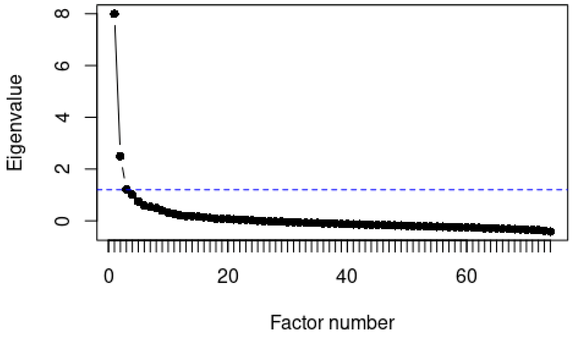
2.3. Factor Analysis

| monomorai | oyayubi | shimoyake | shiasatte | kooru | toomorokoshi | ||
|---|---|---|---|---|---|---|---|
| Kesennuma | Akitakata | 0.86 | 0.29 | 0.25 | 0.40 | 0.67 | 0.63 |
| Kitahiroshima | Akitakata | 0.00 | 0.00 | 0.00 | 0.13 | 0.67 | 0.80 |
| Kitahiroshima | Kesennuma | 0.86 | 0.29 | 0.25 | 0.36 | 0.00 | 0.00 |
| Motoyoshi | Akitakata | 0.86 | 0.29 | 0.25 | 0.40 | 0.63 | 0.63 |
| Motoyoshi | Kesennuma | 0.00 | 0.00 | 0.00 | 0.00 | 0.63 | 0.43 |
| Motoyoshi | Kitahiroshima | 0.86 | 0.29 | 0.25 | 0.36 | 0.63 | 0.89 |
| Setouchi | Akitakata | 0.71 | 0.43 | 0.50 | 0.80 | 0.50 | 0.63 |
| Setouchi | Kesennuma | 0.80 | 0.71 | 0.60 | 0.70 | 0.88 | 0.29 |
| Setouchi | Kitahiroshima | 0.71 | 0.43 | 0.50 | 0.78 | 0.88 | 0.90 |
| Setouchi | Motoyoshi | 0.80 | 0.71 | 0.60 | 0.70 | 0.89 | 0.43 |
| oyayubi | shimoyake | shiasatte | kooru | toomorokoshi | |
|---|---|---|---|---|---|
| monomorai | 0.69 | 0.67 | 0.66 | −0.08 | 0.09 |
| oyayubi | 0.97 | 0.87 | 0.39 | −0.41 | |
| shimoyake | 0.96 | 0.37 | −0.30 | ||
| shiasatte | 0.32 | −0.11 | |||
| kooru | −0.46 |
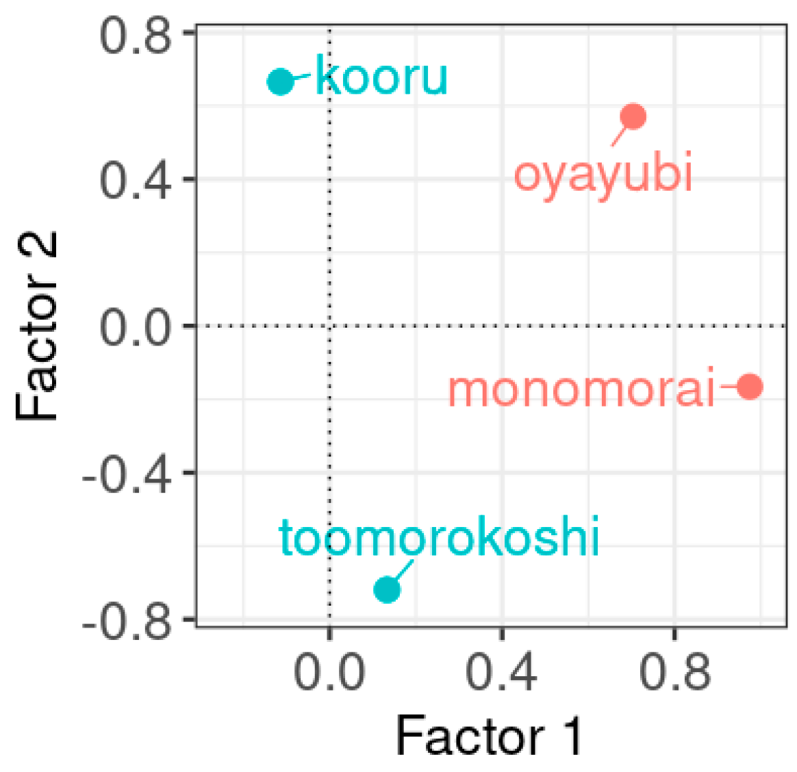
| Factor 1 | Factor 2 | |
|---|---|---|
| monomorai | 0.974 | −0.165 |
| oyayubi | 0.704 | 0.571 |
| kooru | −0.114 | 0.666 |
| toomorokoshi | 0.133 | −0.720 |
a factor analysis only models patterns of variation that are shared by the variables in the dataset, whereas a principal component analysis model totals variation, including variation that is unique to a single variable. A factor analysis is thus the more appropriate technique for identifying common patterns of regional variation and is also less likely to be affected by noise.
2.4. Finding Dialect Areas
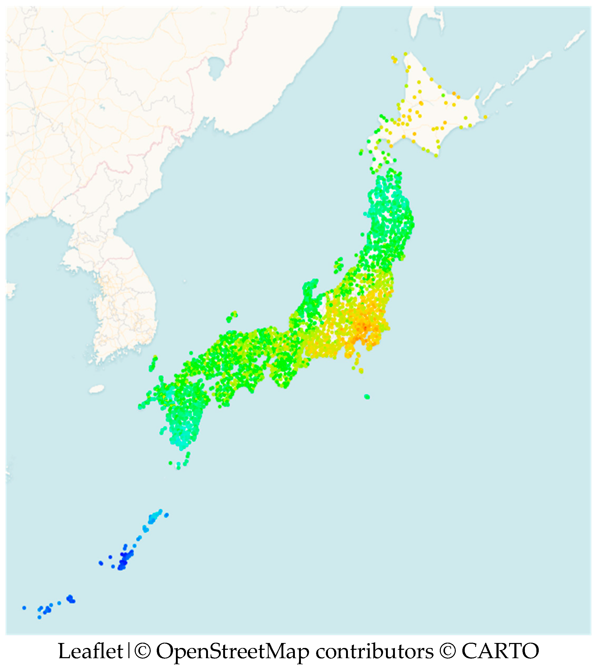
2.5. Visualizing the Dialect Landscape from the Perspective of a Reference Point
3. Unraveling the Big Picture of LAJ by Factor Analysis of Levenshtein Distance
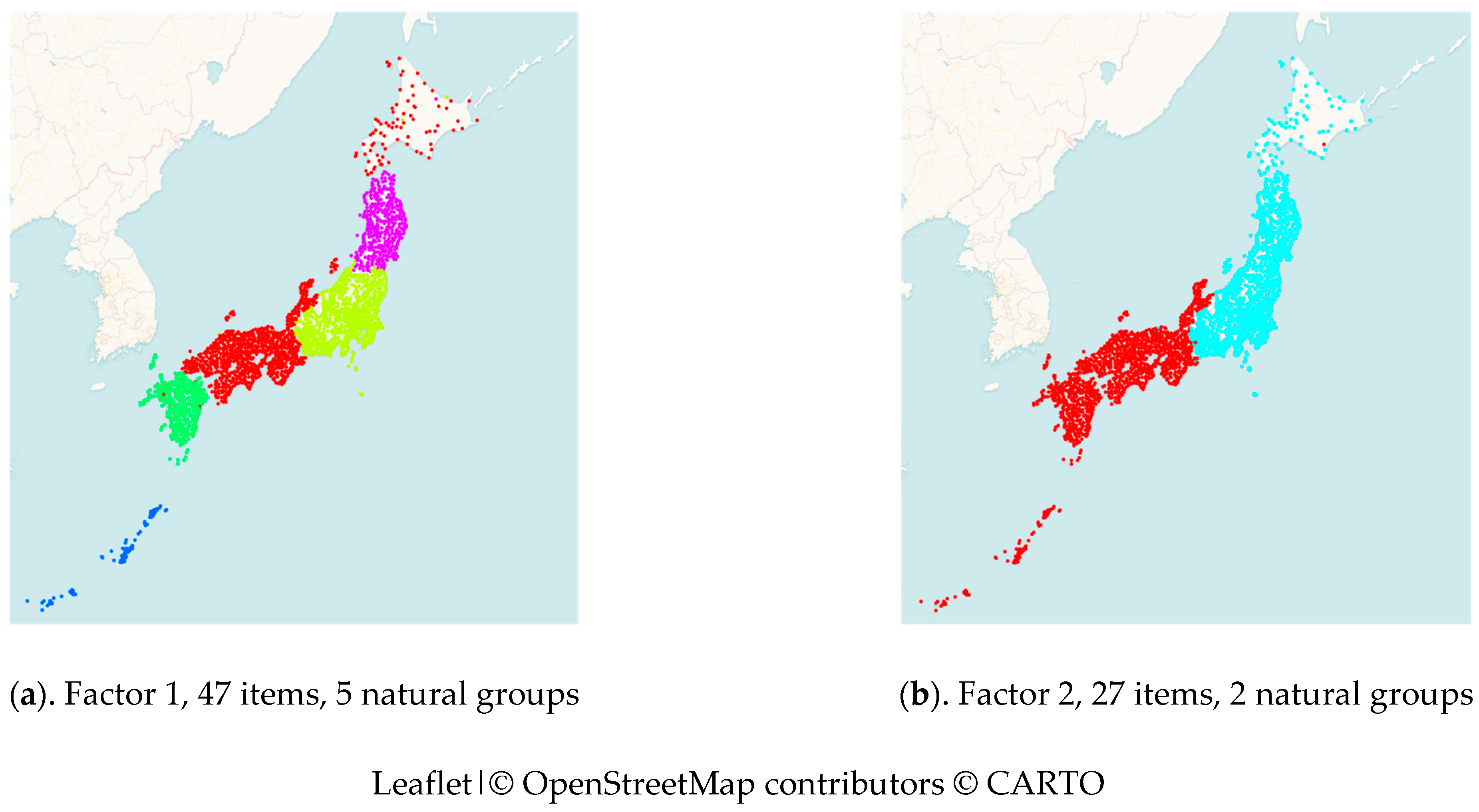
3.1. Finding the Latent Linguistic Variables of Word Forms and Geography
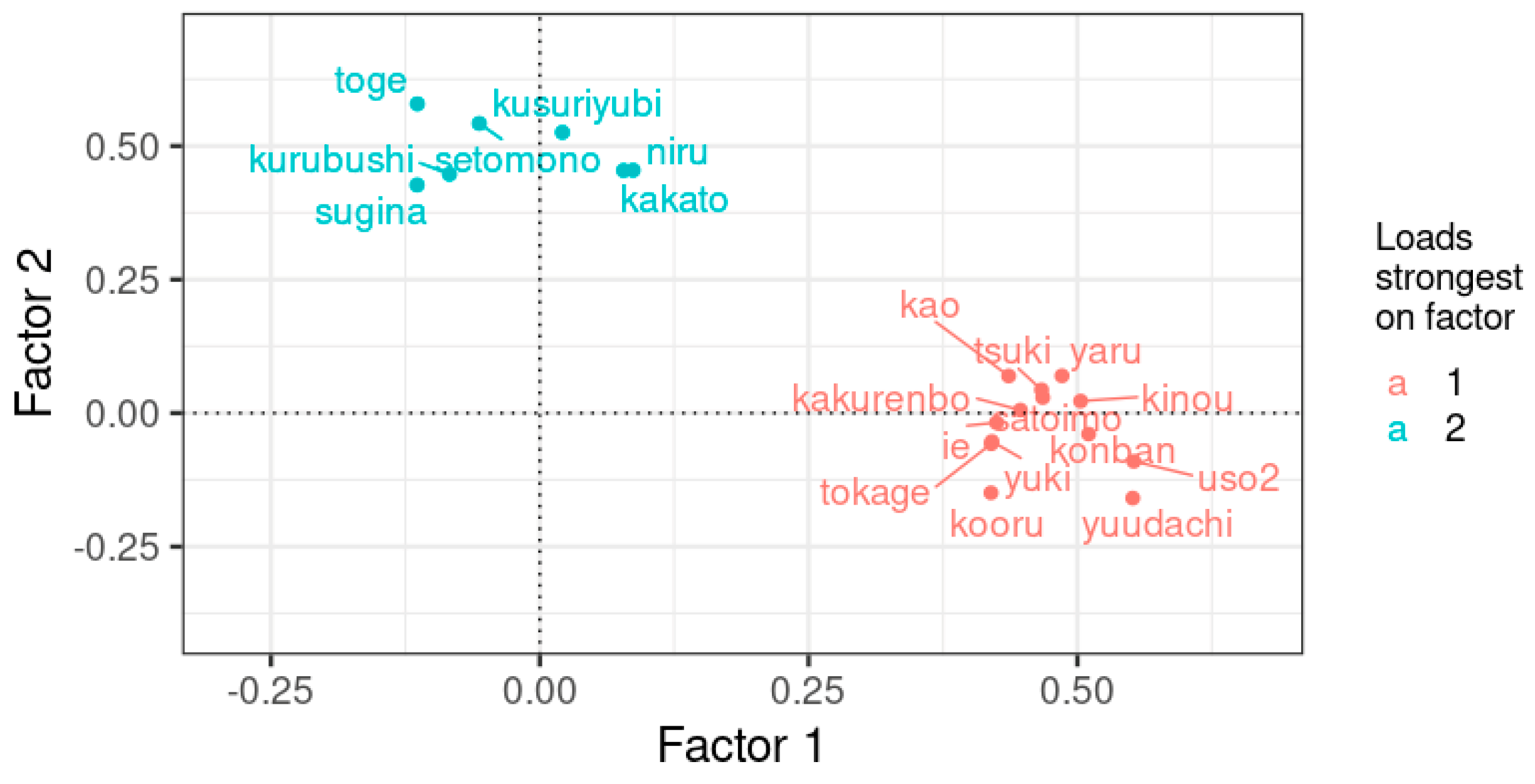
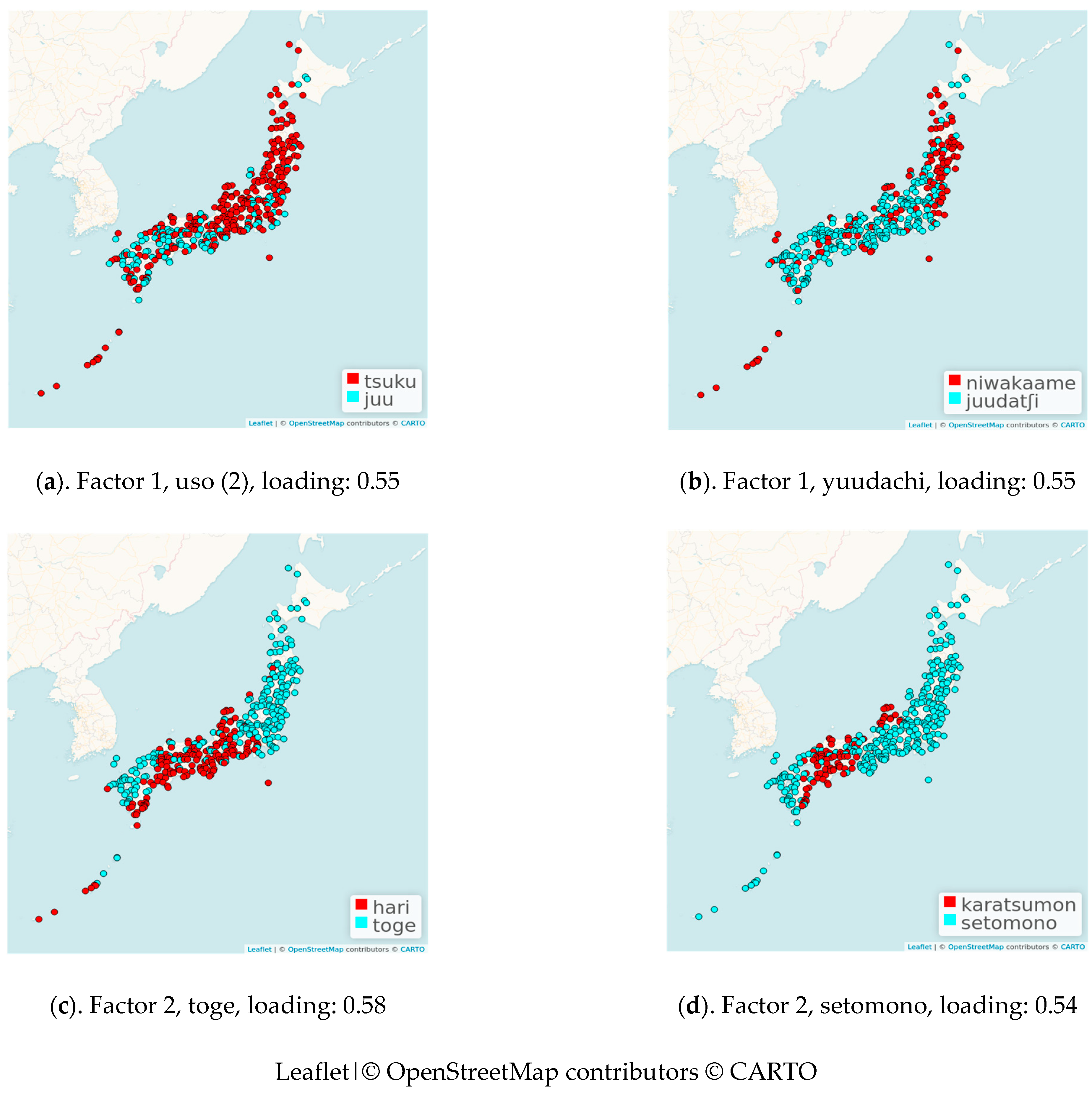
3.2. Examining the Original Variables of Word Forms
4. Unraveling the Latent Linguistic Variables with Tokyo as a Reference Point
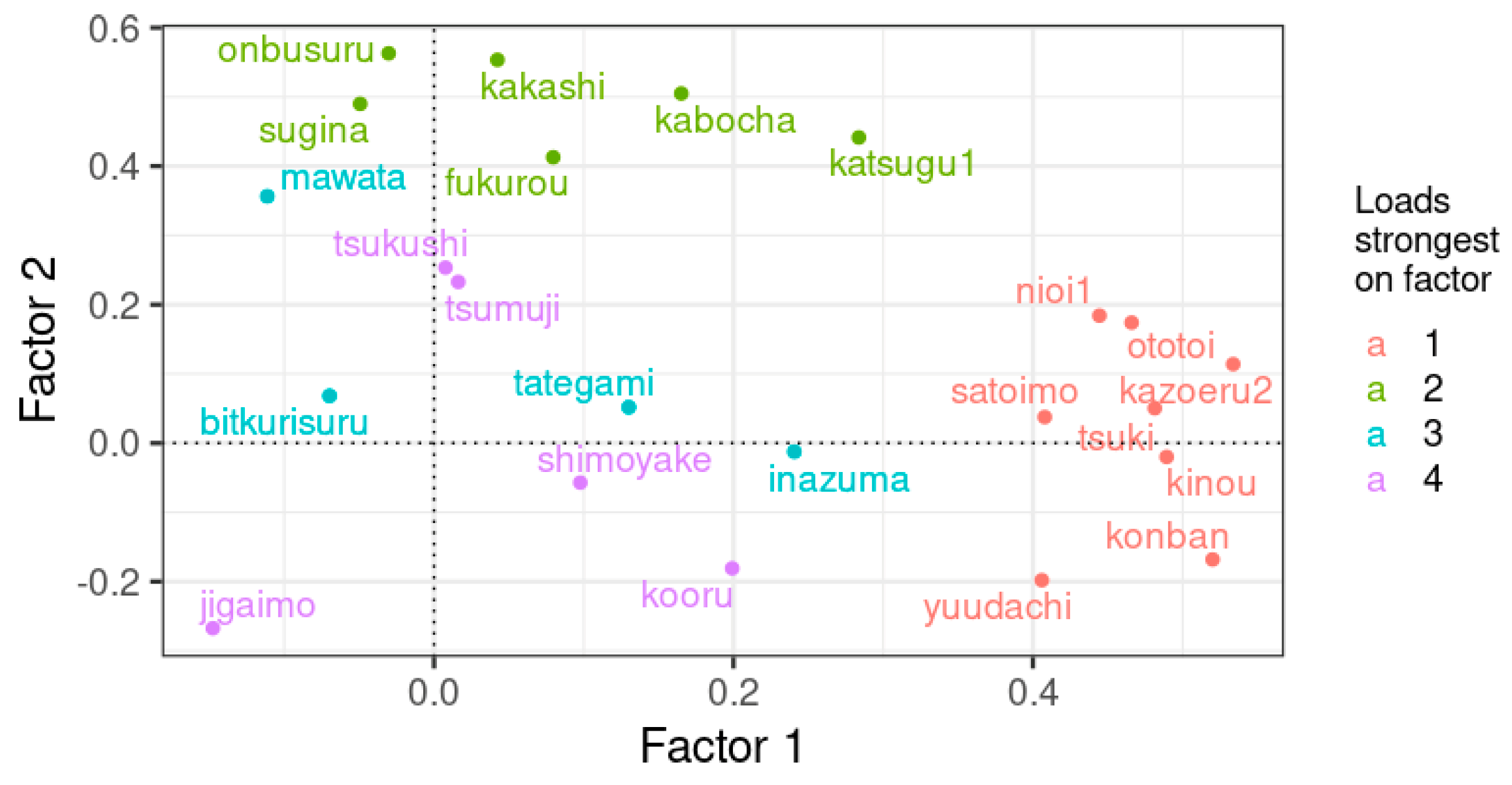
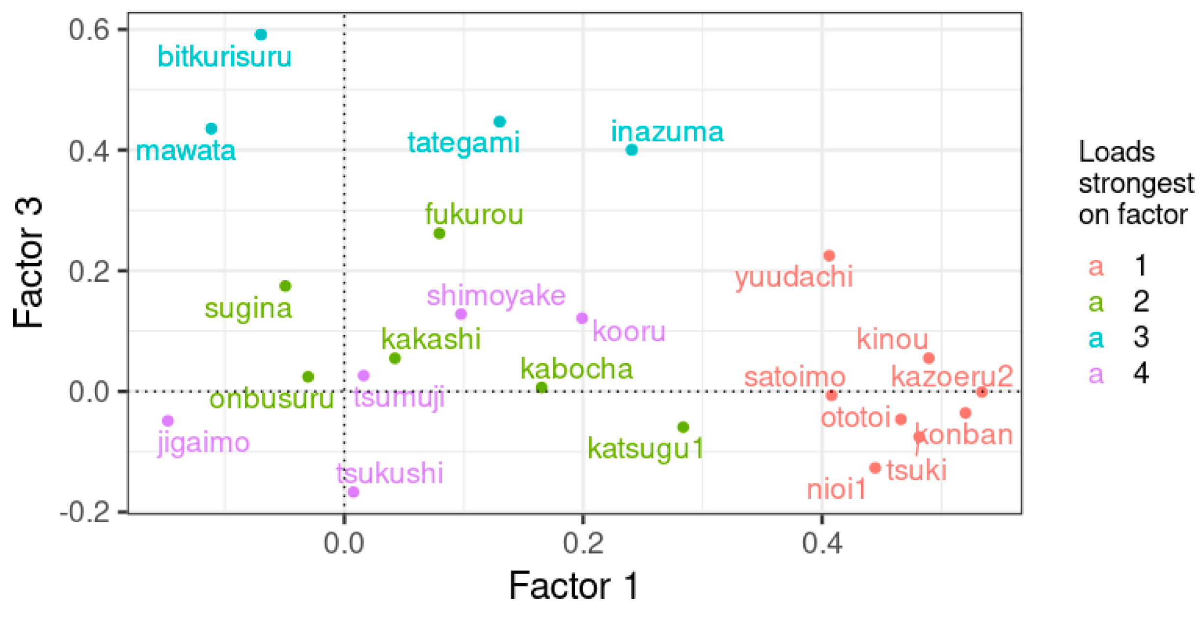
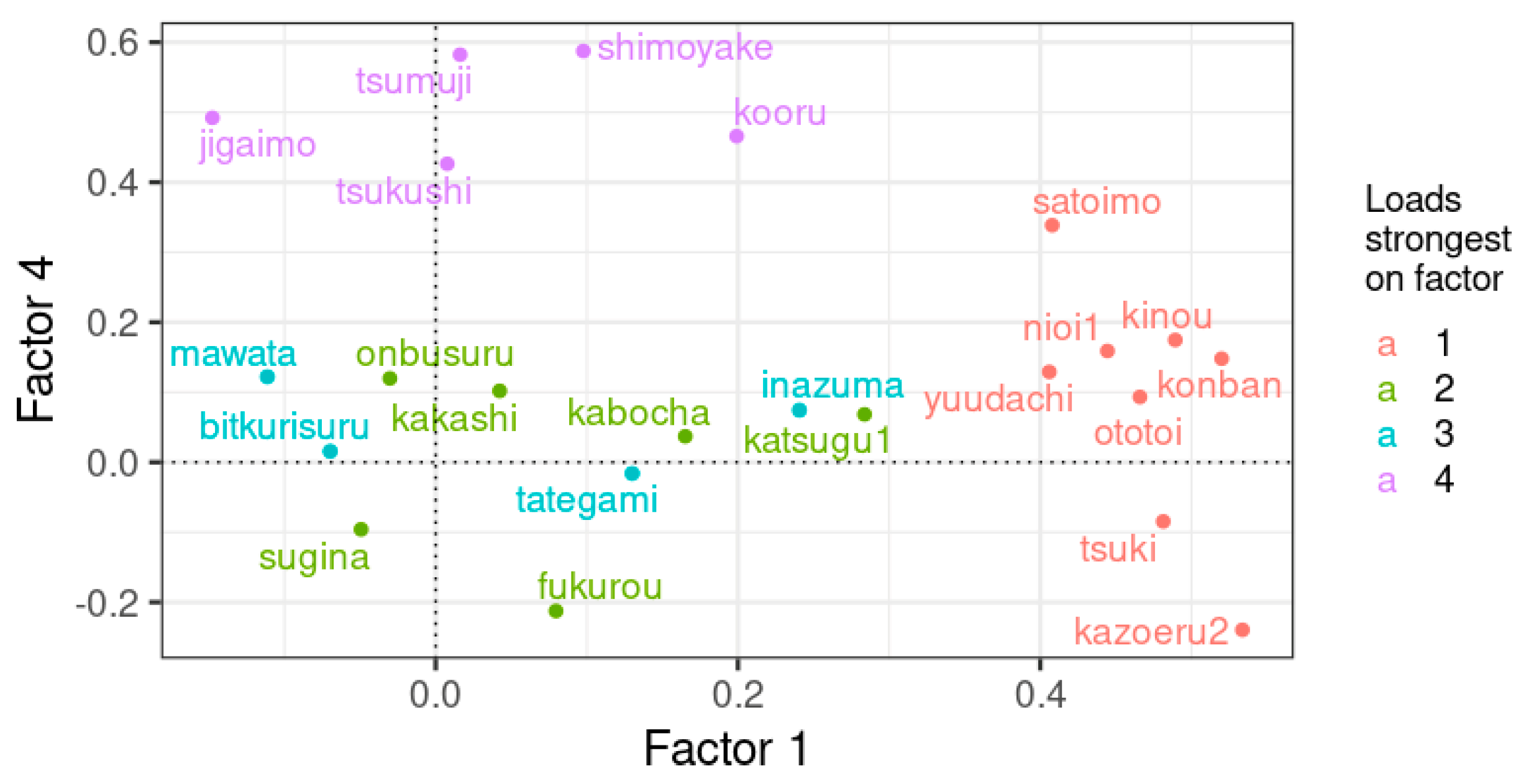
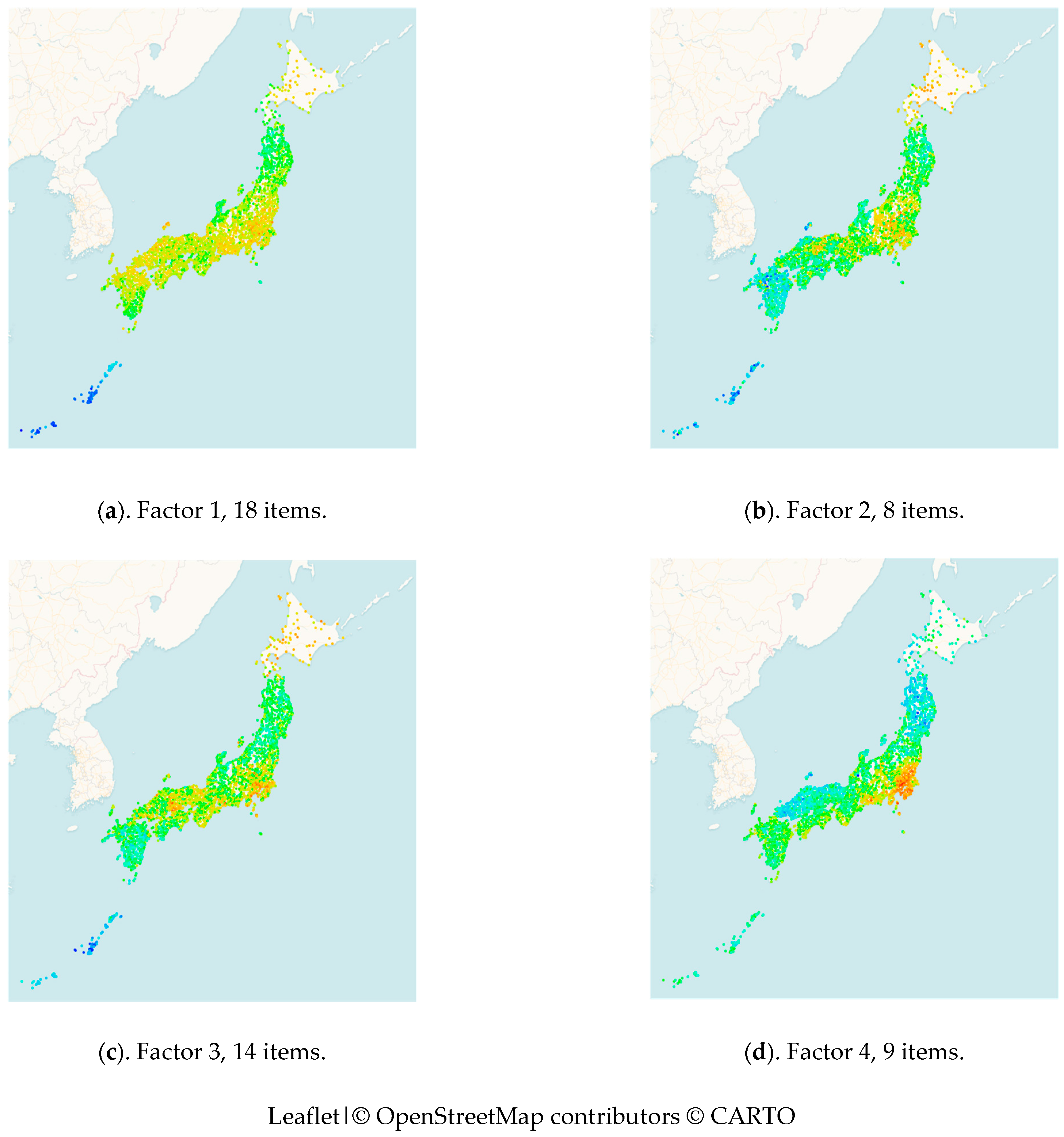
4.1. Finding the Latent Linguistic Variables with Tokyo as a Reference Point
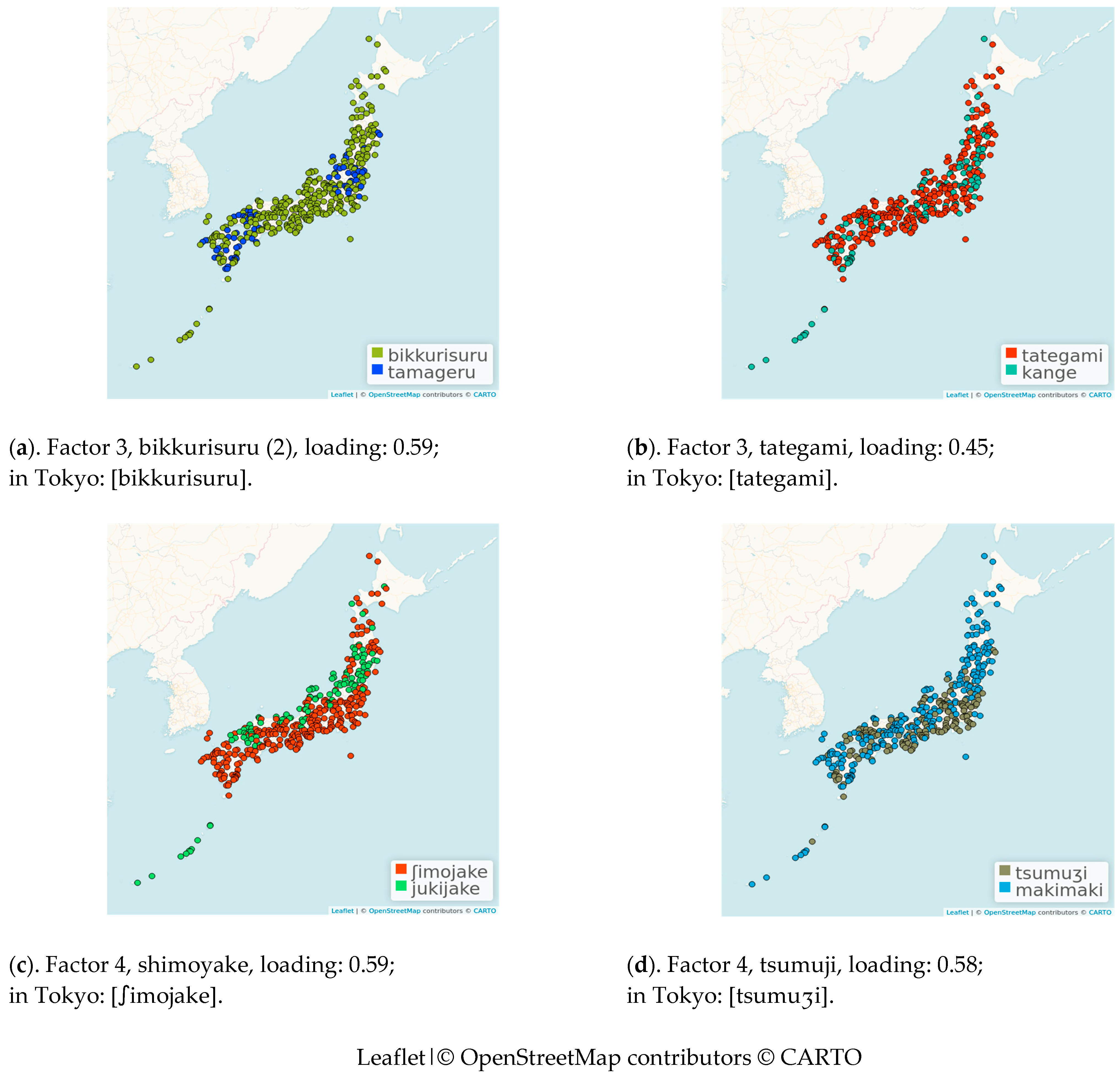
4.2. Examining the Original Variables with Tokyo as a Reference Point
5. The Influence of Tokyo on the Japanese Dialects
5.1. Is Tokyo the Most Influential Dialect?
5.2. Which Local Dialects Are Particularly Influenced by the Tokyo Dialect?
6. Discussions and Conclusions
6.1. Direct Results of LAJ
6.2. Evaluation of the Factor Analyses
6.3. Comparison to Earlier Works of LAJ
Author Contributions
Funding
Institutional Review Board Statement
Informed Consent Statement
Data Availability Statement
Acknowledgments
Conflicts of Interest
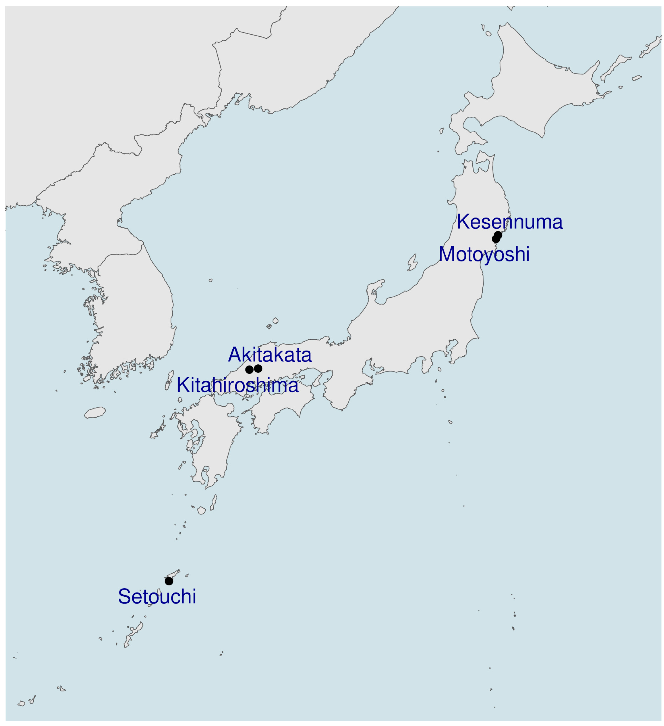
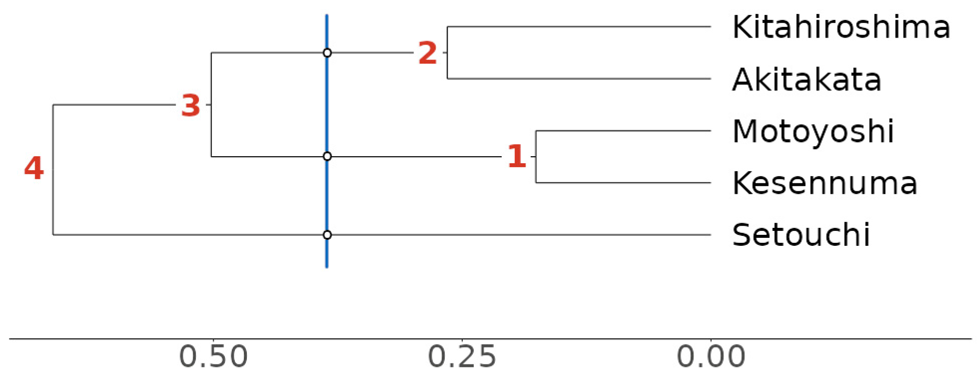
| 1 | Since 2009, Motoyoshi no longer exists as an independent city, but has been merged into the expanded city of Kesennuma. |
| 2 | Respectively codes 4716.20 and 0257.12 in the LAJDB. |
| 3 | |
| 4 | |
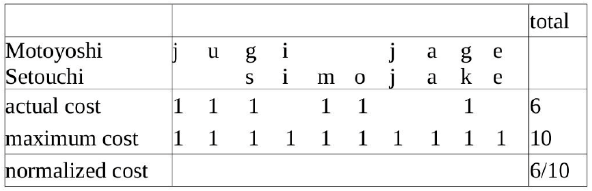
| 5 | In this example we used transcriptions from LAJDB. Since this example data set is small, it is not possible to learn the weights well using PMI Levenshtein distance. We therefore applied plain Levenshtein distance where insertions, deletions and substitutions have a weight of 1, as we did in Figure 1 and Table 2. |
| 6 | Since we are only giving an example here, we will continue with the analysis. |
| 7 | The LAJDB codes of the locations are 4706.53 (Kesennuma), 4716.20 (Motoyoshi), 6450.45 (Atikata), 6359.62 (Kitahiroshima), and 0257.12 (Setouchi). |
| 8 | For more information about this procedure see https://statsandr.com/blog/files/Hierarchical-clustering-cheatsheet.pdf (accessed on 23 May 2025). This procedure is implemented in LED-A. |
| 9 | For the two groups we found Cronbach’s α values of 0.8765 and 0.8776. A widely accepted threshold is 0.70 (Nunnally, 1978), therefore the number of items was sufficient in order to produce reliable results. |
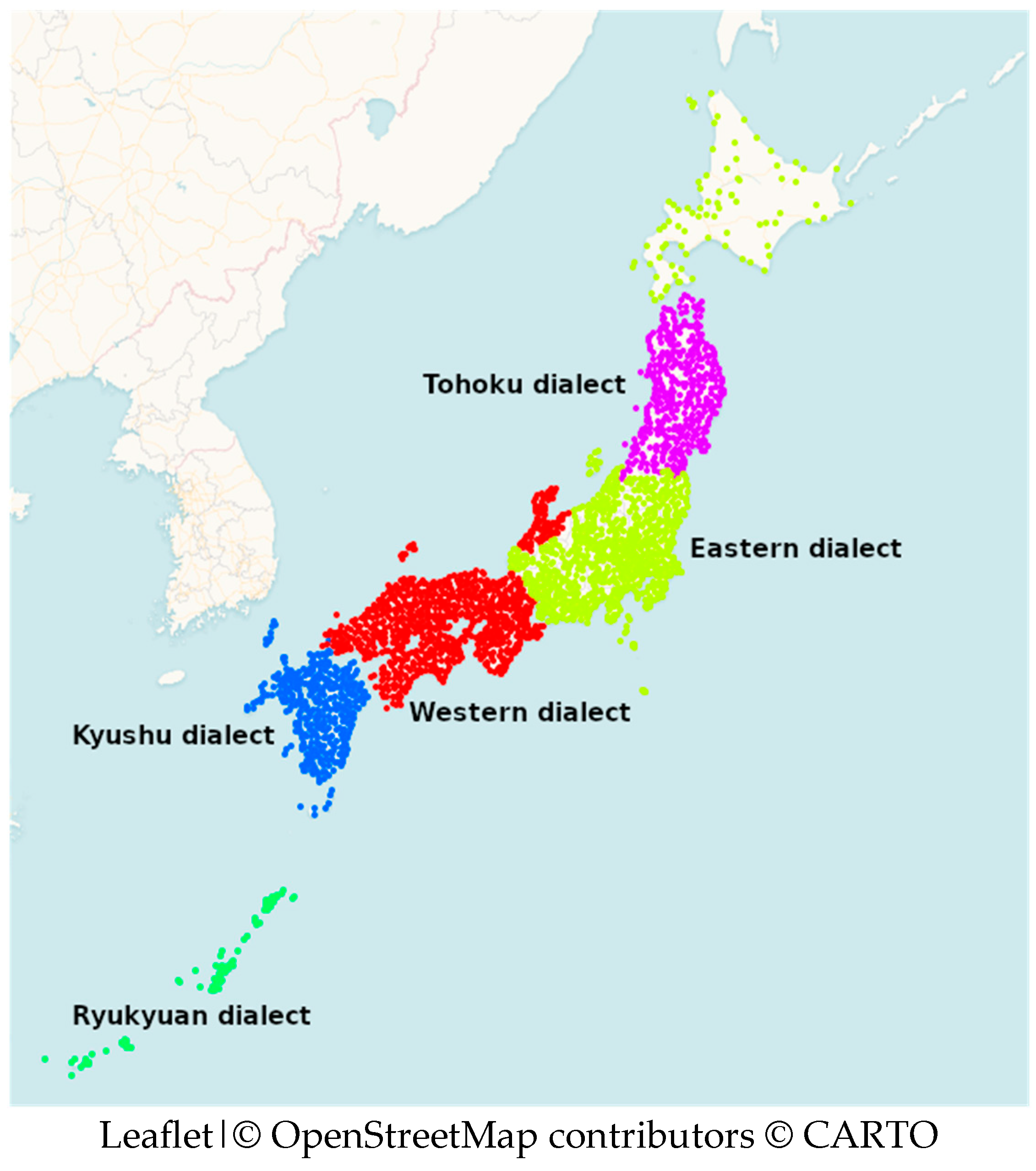
| 10 | The maps give a general idea of the variation of the items across the regions so that the reader can develop an idea of the basis for the division into areas, but should by no means be seen as a substitute for the much more precise and accurate maps in the LAJ. |
| 11 | In the LAJDB all localities are represented by codes. We determined location 5698.69 closest to Tokyo just by eyeballing. |
| 12 | Actually distances among all 2400 sites were calculated, and subsequently the distances to Tokyo were selected from the respective distance matrices. Considering the full datasets the Cronbach’s α values of the four groups are, respectively, 0.7738, 0.6518, 0.6738 and 0.3864. Since three coefficients are (slightly) lower than the threshold of 0.70 (see Section 2.2) the results should be interpreted with care. |
| 13 | We emphasize again that these maps are a highly simplified representation, the number of different forms in the original LAJ maps is always much larger. |
| 14 | [juki] means “snow” and [ʃimo] means “frost”. |
| 15 | In the LAJDB this location has code 1719.17. Historically, Nagayama was an independent town but merged with Asahikawa in 1961, becoming one of its districts. |
| 16 | The function distHaversine() from the R package geosphere (Hijmans, 2024) was used, see also Sinnott (1984). |
| 17 | We used the function gam from the R package mgcv (Wood, 2011). |
| 18 | We obtained a lower adjusted R-square value of 0.4912 when using a linear regression model. When using logarithmic geographic distances, the adjusted R-square dropped to 0.4648, and when using the square root of the geographic distance, we obtained a higher value of 0.5005. |
| 19 | We used the function find_route() from the R package osrm which retrieves these data from Open Street Map. |
| 20 | In the LAJDB this location has code 0896.22. Originally an independent town, Tokoro merged with Kitami in 2006. |
References
- Bolognesi, R., & Heeringa, W. (2002). De invloed van dominante talen op het lexicon en de fonologie van Sardische dialecten [The influence of dominant languages on the lexicon and phonology of Sardinian dialects]. Gramma/TTT: Tijdschrift voor taalwetenschap, 9(1), 45–84. Available online: http://www.wjheeringa.nl/papers/rom01.pdf (accessed on 23 May 2025).
- Cattell, R. B. (1966). The scree test for the number of factors. Multivariate Behavioral Research, 1(2), 245–276. [Google Scholar] [CrossRef] [PubMed]
- Cronbach, L. J. (1951). Coefficient alpha and the internal structure of tests. Psychometrika, 16, 297–334. Available online: http://cda.psych.uiuc.edu/psychometrika_highly_cited_articles/cronbach_1951.pdf (accessed on 23 May 2025). [CrossRef]
- Field, A., Miles, J., & Field, Z. (2012). Discovering statistics using R. Sage. [Google Scholar]
- Fujiwara, Y. (1990). Nihongo hogen bunpa ron [Dialect propagation theory of Japanese]. Musashino Shoin. [Google Scholar]
- Gere, A. (2023). Recommendations for validating hierarchical clustering in consumer sensory projects. Current Research in Food Science, 6, 100522. [Google Scholar] [CrossRef]
- Goebl, H. (1981). Eléments d’analyse dialectométrique (avec application à l’ais). Revue de Linguistique Romane, 45, 349–420. [Google Scholar]
- Goebl, H. (2002). Analyse dialectométrique des structures de profondeur de l’ALF. Revue de Linguistique Romane, 66(261–262), 5–63. [Google Scholar]
- Grieve, J. (2014). A comparison of statistical methods for the aggregation of regional linguistic variation. In B. Szmrecsanyi, & B. Wälchli (Eds.), Aggregating dialectology, typology, and register analysis: Linguistic variation in text and speech (pp. 53–88). De Gruyter. [Google Scholar] [CrossRef]
- Heeringa, W. (2004). Measuring dialect pronunciation differences using levenshtein distance [Unpublished doctoral dissertation, University of Groningen]. Available online: http://www.wjheeringa.nl/thesis/ (accessed on 23 May 2025).
- Heeringa, W., & Inoue, F. (2023). Exploring the Japanese dialect geography dialectometrically: Division and continuity. Studies in Geolinguistics, 3, 1–44. [Google Scholar] [CrossRef]
- Hijmans, R. (2024). _geosphere: Spherical trigonometry_. R package version 1.5-20. Available online: https://CRAN.R-project.org/package=geosphere (accessed on 3 April 2025).
- Horn, J. L. (1965). A rationale and test for the number of factors in factor analysis. Psychometrika, 30(2), 179–185. [Google Scholar] [CrossRef]
- Huisman, J. L. A. (2021). Variation in form and meaning across the Japonic language family: With a focus on the Ryukyuan languages [Doctoral dissertation, Radboud University Nijmegen]. Available online: https://pure.mpg.de/rest/items/item_3311139/component/file_3311141/content (accessed on 23 May 2025).
- Huisman, J. L. A., Majid, A., & van Hout, R. (2019). The geographical configuration of a language area influences linguistic diversity. PLoS ONE, 14(6), e0217363. [Google Scholar] [CrossRef]
- Inoue, F. (2001). Keiryoteki hogen kukaku [Quantificational dialect classification]. Meiji Shoin. [Google Scholar]
- Inoue, F. (2010). Real and apparent time clues to the speed of dialect diffusion. Dialectologia: Revista Electrònica, 2010(5), 45–64. [Google Scholar]
- Inoue, F., & Hanzawa, Y. (2024). New dialect and obsolescence in hamaogi glottogram survey―Dialect vocabulary change in 250 years. Dialectologia: Revista Electrònica, 32, 47–116. [Google Scholar]
- Inoue, F., & Kasai, H. (1989). Dialect classification by standard Japanese forms. Japanese Quantitative Linguistics, 39, 220–235. [Google Scholar]
- Inoue, F., & Yarimizu, K. (2024). Language standardization and railway-walking distance–Levenshtein distance and distribution in GAJ. Dialectologia et Geolinguistica, 32, 79–97. [Google Scholar] [CrossRef]
- Jain, A. K., & Dubes, R. C. (1988). Algorithms for clustering data. Prentice Hall. [Google Scholar]
- Jeszenszky, P., Hikosaka, Y., Imamura, S., & Yano, K. (2019). Japanese lexical variation explained by spatial contact patterns. ISPRS International Journal of Geo-Information, 8(9), 400. [Google Scholar] [CrossRef]
- Jolliffe, P. M. (2020). Forced Labour in Imperial Japan’s First Colony: Hokkaidō. The Asia–Pacific Journal, 18(20), e7. [Google Scholar] [CrossRef]
- Kessler, B. (1995, March 27–31). Computational dialectology in Irish Gaelic. 7th Conference of the European Chapter of the Association for Computational Linguistics (pp. 60–67), Dublin, Ireland. Available online: https://arxiv.org/pdf/cmp-lg/9503002.pdf (accessed on 23 May 2025).
- Kumagai, Y. (2016). Developing the linguistic atlas of Japan database and advancing analysis of geographical distributions of dialects. In M.-H. Côté, R. Knooihuizen, & J. Nerbonne (Eds.), The future of dialects. Selected papers from methods in dialectology XV (= Language Variation 1) (pp. 333–362). Language Science Press. [Google Scholar]
- Mason, M. (2012). Dominant narratives of colonial Hokkaido and imperial Japan: Envisioning the periphery and the modern nation-state (pp. 7–9). Palgrave Macmillan. [Google Scholar]
- Nerbonne, J. (2006). Identifying linguistic structure in aggregate comparison. Literary and Linguistic Computing, 21(4), 463–475. [Google Scholar] [CrossRef]
- Nunnally, J. C. (1978). Psychometric theory. McGraw-Hill. [Google Scholar]
- Nunnally, J. C., & Bernstein, I. H. (1994). Psychometric theory (3rd ed.). McGraw-Hill. [Google Scholar]
- Onishi, T. (2019). On the relationship of the degrees of correspondence of dialects and distances. Languages, 4(2), 37. [Google Scholar] [CrossRef]
- Pickl, S., & Pröll, S. (2019). Geolinguistische querschnitte und tiefenbohrungen in bayern und darüber hinaus. In Methodik moderner Dialektforschung. Erhebung, Aufbereitung und Auswertung von Daten am Beispiel des Oberdeutschen (pp. 141–143). Georg Olms Verlag. [Google Scholar]
- Shibatani, M. (1990). The languages of Japan. Cambridge University Press. [Google Scholar]
- Sinnott, R. W. (1984). Virtues of the haversine. Sky and Telescope, 68(2), 159. [Google Scholar]
- Van der Maaten, L. (2014). Accelerating t-SNE using tree-based algorithms. Journal of Machine Learning Research, 15, 3221–3245. Available online: https://www.jmlr.org/papers/volume15/vandermaaten14a/vandermaaten14a.pdf (accessed on 23 May 2025).
- Van der Maaten, L., & Hinton, G. (2008). Visualizing data using t-SNE. Journal of Machine Learning Research, 9, 2579–2605. Available online: https://www.jmlr.org/papers/volume9/vandermaaten08a/vandermaaten08a.pdf (accessed on 23 May 2025).
- Ward, J. H., Jr. (1963). Hierarchical grouping to optimize an objective function. Journal of the American Statistical Association, 58, 236–244. [Google Scholar] [CrossRef]
- Wieling, M. (2012). A quantitative approach to social and geographical dialect variation [Doctoral dissertation, University of Groningen]. Available online: https://hdl.handle.net/11370/cd637817-572f-4826-98c1-08272775fb64 (accessed on 23 May 2025).
- Wieling, M., Prokić, J., & Nerbonne, J. (2009). Evaluating the pairwise alignment of pronunciations. In L. Borin, & P. Lendvai (Eds.), Proceedings of the EACL 2009 workshop on language technology and resources for cultural heritage, social sciences, humanities, and Education, (LaTeCH–SHELT&R 2009). Workshop at the 12th meeting of the European chapter of the association for computational linguistics. Athens, 30 March 2009 (pp. 26–34). Association for Computational Linguistics (ACL). Available online: https://aclanthology.org/W09-0304.pdf (accessed on 23 May 2025).
- Wood, S. N. (2011). Fast stable restricted maximum likelihood and marginal likelihood estimation of semiparametric generalized linear models. Journal of the Royal Statistical Society Series B, 73(1), 3–36. [Google Scholar] [CrossRef]
- Yarimizu, K. (2007). Hogen bunpo zenkoku chizu ni okeru kyotsugoka no jokyo (The situation of common language in GAJ). Nihongogaku, 26(11), 112–119. [Google Scholar]


| Code | Japanese | Hepburn Romanization | Transcription of Tokyo | Meaning in English |
|---|---|---|---|---|
| 1 | かまきり(蟷螂) | kamakiri | KAGAMICCYO, TOOROO(MUSI), HARATACIGONBE(E) | mantis |
| 2 | くも(蜘蛛) | kumo | spider | |
| 3 | くものいと(蜘蛛の糸) | kumonoito | spider thread | |
| 4 | くものす(蜘蛛の巣) | kumonosu | spider web | |
| 5 | かたつむり(蝸牛) | katatsumuri | MAIMAICUBURO, KATACUMURI | snail |
| 6 | なめくじ(蛞蝓) | namekuji | NAMEKUZI | slug |
| 7 | おたまじゃくし(蝌蚪) | otamajakushi | OTAMAZYAKUSI | tadpole |
| 8 | かえる(蛙) | kaeru | KAERU | frog |
| 12 | とかげ(蜥蜴) | tokage | TOKAGE | lizard |
| 21-7 月 | うそ(嘘言)をつく ---前部分 | uso 1 | to tell a lie–front part | |
| 21-8 月 | うそ(嘘言)をつく ---後部分 | uso 2 | to tell a lie–back part | |
| 23 | つくる(作る) | tsukuru | to make | |
| 31 | あたま(頭) | atama | head | |
| 32 | つむじ(旋毛) | tsumuji | CUMUZI | whirlpool |
| 34 | め(目) | me | eye | |
| 36 | ものもらい(麦粒腫) | monomorai | MONOMORAI | sty in the eye |
| 37 | はな(鼻) | hana | nose | |
| 38 | におい(芳香) | nioi 1 | NIOI | scent (aroma) |
| 39 | におい(悪臭) | nioi 2 | NIOI | odor (bad smell) |
| 7 月-42 | におい(匂)をかぐ(嗅ぐ) | nioi 3 | NIOI O--- | to smell |
| 8 月-42 | におい(匂)をかぐ(嗅ぐ) | nioi 4 | (---)KAGU | to smell |
| 44 | くち(口) | kuchi | mouth | |
| 47 | くちびる(唇) | kuchibiru | KUCIBIRU | lips |
| 48 | した(舌) | shita | SITA, BERO | tongue |
| 51 | 〈塩味が〉うすい | usui | AMAI | lightly salty |
| 52 | あまい(甘い) | amai | AMAI | sweet |
| 56 | ほほ(頬) | hoho | HOO | cheek |
| 57 | かお(顔) | kao | KAO | face |
| 59 | あざ(痣)になる | aza | AZA・NI NARU, AZA---DEKIRU | to get a bruise |
| 60 | ほくろ(黒子)—小さいもの | hokuro 1 | HOKORO | mole–small |
| 61 | ほくろ(黒子)—大きいもの | hokuro 2 | mole–large | |
| 63 | おやゆび(親指) | oyayubi | OYAIBI | thumb |
| 64 | ひとさしゆび(人差し指) | hitosashiyubi | HITOSASIIBI | index finger |
| 65 | なかゆび(中指) | nakayubi | NAKAIBI | middle finger |
| 66 | くすりゆび(薬指) | kusuriyubi | KUSURIIBI | ring finger |
| 67 | こゆび(小指) | koyubi | KOIBI | pinky finger |
| 68 | しもやけ(凍傷) | shimoyake | SIMOYAKE | frostbite |
| 69 | かかと(踵) | kakato | KAKATO | heel |
| 72 | すわる(坐る) | suwaru | KASIKOMARU | to sit |
| 73 | みずおち(鳩尾) | mizuochi | MIZOOCI | pith |
| 74 | あか(垢) | aka | dirt | |
| 75 | ふけ(雲脂) | fuke | dandruff | |
| 76 | うろこ(鱗) | uroko | KOKE, KOKERA | scales |
| 79 | きのこ(茸・蕈) | kinoko | KINOKO | mushroom |
| 80 | おとこ(男) | otoko | man | |
| 81 | おんな(女) | onna | woman | |
| 83 | たけうま(竹馬) | takeuma | TAKENMA | stilts |
| 89 | かくれんぼ(隠れん坊) | kakurenbo | KAKURENBO | hide-seek |
| 90 | おかね(貨幣) | okane | OKANE, OASI | money |
| 91 | おつり(釣銭) | otsuri | small changes | |
| 92 | かぞえる(お金を数える) | kazoeru 1 | to count (money) | |
| 93 | かぞえる(数える) | kazoeru 2 | KAZOERU | to count |
| 95 | やる(遣る) | yaru | YARU | to give |
| 102 | きょう(今日) | kyoo | today | |
| 103 | きのう(昨日) | kinoo | KINOO | yesterday |
| 104 | おととい(一昨日) | ototoi | OTOTOI | the day before yesterday |
| 105 | さきおととい(一昨昨日) | sakiototoi | SAKIOTOTOI | the two days before yesterday |
| 108 | あした(明日) | ashita | tomorrow | |
| 109 | あさって(明後日) | asatte | the day after tomorrow | |
| 110 | しあさって(明明後日) | shiasatte | SIASATTE | the two days after tomorrow |
| 111 | やのあさって(明明明後日) | yanoasatte | YANOASATTE | the three days after tomorrow |
| 112 | こんばん(今晩) | konban | KON’YA | tonight |
| 113 | あしたのばん(明晩) | ashitanoban | tomorrow night | |
| 114 | たいよう(太陽) | taiyoo | OTENTOOSAMA | sun |
| 116 | つき(月) | tsuki | OCUKISAMA | moon |
| 117 | あめ(雨) | ame | rain | |
| 118 | つゆ(梅雨) | tsuyu | CUYU, NYUUBAI | rainy season |
| 119 | ゆうだち(夕立雨) | yuudachi | YUUDACI | evening shower |
| 122 | いなずま(稲妻・電光) | inazuma | INABIKARI | lightning, electric flash |
| 124 | にじ(虹) | niji | NIZI | rainbow |
| 125 | ゆき(雪) | yuki | snow | |
| 127 | こおる(水が凍る) | kooru | KOORU | to freeze (water freezes) |
| 129 | つらら(氷柱) | tsurara | CURARA | icicle |
| 131 | ごみ(目にはいるもの—塵) | gomi 1 | something that gets into your eye–dust | |
| 132 | ごみ(掃除の対象—塵芥) | gomi 2 | something to clean up–rubbish | |
| 134 | ごみ(川のごみ—塵芥) | gomi 3 | river waste | |
| 135 | じしん(地震) | jishin | earthquake | |
| 148 | たく(炊く) | taku | TAKU | to cook |
| 149 | にる(煮る) | niru | NIRU | to boil |
| 153 | ゆげ(蒸気—飯の場合) | yuge | YUGE | steam - in the case of rice |
| 155 | すりばち(擂鉢) | suribachi | mortar | |
| 156 | すりこぎ(擂粉木) | surikogi | mortar wood | |
| 157 | せともの(陶磁器) | setomono | ceramics | |
| 164 | わた(綿) | wata | WATA | cotton |
| 165 | まわた(真綿) | mawata | MAWATA | floss |
| 166 | いと(糸) | ito | ITO | thread |
| 167 | きぬいと(絹糸) | kinuito | silk thread | |
| 169 | はたいと(機糸) | hataito | machine thread | |
| 173 | こめ(米) | kome | rice | |
| 174 | うるち(粳米) | uruchi | URUCI | non-glutinous rice |
| 176 | はんまい(飯米) | hanmai | rice for cooking | |
| 179 | ぬか(糠) | nuka | NUKA | bran |
| 182 | あぜ(畦畔) | aze | AZE, TANOKURO | ridge |
| 184 | とりおどし(鳥威) | toriodoshi | bird’s threat | |
| 185 | かかし(案山子) | kakashi | KAKASI | scarecrow |
| 186 | じゃがいも(馬鈴薯) | jagaimo | ZYAGAIMO | potato |
| 187 | さといも(里芋) | satoimo | SATOIMO | taro root |
| 188 | さつまいも(甘藷) | satsumaimo | SACUMAIMO | sweet potato |
| 190 | とうもろこし(玉蜀黍) | toomorokoshi | TOOMOROKOSI | corn |
| 191 | かぼちゃ(南瓜) | kabocha | KABOCYA, TOONASU | pumpkin |
| 192 | すみれ(菫) | sumire | violet | |
| 194 | つくし(土筆) | tsukushi | CUKUSI(N)BO(O) | horsetail |
| 195 | すぎな(杉菜・間荊) | sugina | SUGINA | field horsetail (Equisetum arvense) |
| 197 | まつかさ(松毬) | matsukasa | MACUBOKKURI | pine cone |
| 200 | とげ(刺・棘)—いばらやさんしょうなどのとげ | toge | TOGE | thorn |
| 213 | うま(馬) | uma | NMA | horse |
| 214 | おうま(牡馬) | ouma | stalion | |
| 215 | めうま(牝馬) | meuma | mare | |
| 216 | こうま(子馬) | kouma | foal | |
| 217 | たてがみ(鬣) | tategami | TATEGAMI | mane |
| 218 | うし(牛) | ushi | USI | cow |
| 219 | おうし(牡牛) | oushi | bull | |
| 220 | めうし(牝牛) | meushi | cow | |
| 221 | こうし(子牛) | koushi | calf | |
| 222 | もうもう(牛の鳴き声) | moumou | cow mooing | |
| 223 | もぐら(土竜・〓鼠) | mogura | MOGURA | mole |
| 224 | ふくろう(梟) | fukurou | HUKUROO | owl |
| 228 | すずめ(雀) | suzume | sparrow | |
| 229 | ちゅんちゅん(雀の鳴き声) | chunchun | the sound of a sparrow | |
| 231 | はげる(禿げる) | hageru | bald | |
| 233 | くるぶし(踝) | kurubushi | KUROBUSI | ankle |
| 235 | すてる(捨てる) | suteru | UCCYARU | throw away |
| 236 | びっくりする(驚く) | bikkurisuru | BIKKURI SURU | be surprised |
| 237 | おそろしい(恐ろしい) | osoroshii | KOWAI | scary |
| 238 | なのか(七日) | nanoka | NANOKA | seventh day |
| 239 | ここのか(九日) | kokonoka | KOKONOKA | ninth day |
| 240 | ひまご(曾孫) | himago | HIKO | great-grandson |
| 241 | やしゃご(玄孫) | yashago | YASYAGO | great-great-grandson |
| 244 | いえ(家屋) | ie | UCI | house |
| 248 | ふすま(襖障子) | fusuma | HUSUMA | sliding doors |
| 250 | 〈虹が〉きれいだ | kireida | KIREEDA | (the rainbow is) beautiful |
| 252 | とうがらし(蕃椒) | toogarashi | TOOGARASI, TONGARASI | cultivated chili peppers |
| 253 | おいしい(美味しい) | oishii | NMAI | delicious |
| 261 | おんぶする(幼児を負う) | onbusuru | ONBUSURU | carry a child on your back |
| 264 | かつぐ(材木を担ぐ) | katsugu 1 | KACUGU | to carry (timber) |
| 265 | かつぐ(天秤棒を担ぐ) | katsugu 2 | KACUGU | carry a pole |
| 266 | かつぐ(二人で担ぐ) | katsugu 3 | KACUGU | carrying (by two people) |
| 268 | いる(居る) | iru | IRU | (man) is (exists) |
| 270 | 〈いい天気〉だ | da | DA | it’s <nice weather> |
| 282 | なす(茄子) | nasu | NASU | eggplant |
| 284 | とんぼ(蜻蛉) | tonbo | TANBO | dragonfly |
| Word | Meaning in English | Motoyoshi | Setouchi | Cost | Maximum Cost | Normalized Cost |
|---|---|---|---|---|---|---|
| monomorai | sty in the eye | baka | ibiri | 4 | 5 | 0.80 |
| oyayubi | thumb | oojubi | ujajup | 5 | 7 | 0.71 |
| shimoyake | frostbite | jugijage | simojake | 6 | 10 | 0.60 |
| shiasatte | the two days after tomorrow | janoasatte | juhwaa | 7 | 10 | 0.70 |
| kooru | freezes | sugaharu | koojum | 8 | 9 | 0.89 |
| toomorokoshi | corn | toomugi | tookibi | 3 | 7 | 0.43 |
| 4.13/6 = 0.69 |
| Kesennuma | Kitahiroshima | Motoyoshi | Setouchi | |
|---|---|---|---|---|
| Akitakata | 0.51 | 0.27 | 0.51 | 0.60 |
| Kesennuma | 0.44 | 0.18 | 0.66 | |
| Kitahiroshima | 0.55 | 0.70 | ||
| Motoyoshi | 0.69 |
| Item | Meaning in English | Factor 1 | Factor 2 |
|---|---|---|---|
| tokage | lizard | 0.42 | −0.06 |
| uso2 | to tell a lie–back part | 0.55 | −0.09 |
| kao | face | 0.44 | 0.07 |
| kusuriyubi | ring finger | 0.02 | 0.53 |
| kakato | heel | 0.08 | 0.45 |
| kakurenbo | hide−seek | 0.45 | 0.01 |
| yaru | to give | 0.49 | 0.07 |
| kinoo | yesterday | 0.5 | 0.02 |
| konban | tonight | 0.51 | −0.04 |
| tsuki | moon | 0.47 | 0.04 |
| yuudachi | evening shower | 0.55 | −0.16 |
| yuki | snow | 0.42 | −0.05 |
| kooru | to freeze (water freezes) | 0.42 | −0.15 |
| niru | to boil | 0.09 | 0.45 |
| setomono | ceramics | −0.06 | 0.54 |
| satoimo | taro root | 0.47 | 0.03 |
| sugina | field horsetail (Equisetum arvense) | −0.11 | 0.43 |
| toge | thorn | −0.11 | 0.58 |
| kurubushi | ankle | −0.08 | 0.45 |
| ie | house | 0.42 | −0.02 |
| Item | Meaning in English | Factor 1 | Factor 2 | Factor 3 | Factor 4 |
|---|---|---|---|---|---|
| tsumuji | whirlpool | 0.02 | 0.23 | 0.03 | 0.58 |
| nioi1 | scent (aroma) | 0.44 | 0.18 | −0.13 | 0.16 |
| shimoyake | frostbite | 0.1 | −0.06 | 0.13 | 0.59 |
| kazoeru2 | to count | 0.53 | 0.11 | 0 | −0.24 |
| kinou | yesterday | 0.49 | −0.02 | 0.06 | 0.17 |
| ototoi | the day before yesterday | 0.47 | 0.17 | −0.05 | 0.09 |
| konban | tonight | 0.52 | −0.17 | −0.04 | 0.15 |
| tsuki | moon | 0.48 | 0.05 | −0.08 | −0.08 |
| yuudachi | evening shower | 0.41 | −0.2 | 0.23 | 0.13 |
| inazuma | lightning, electric flash | 0.24 | −0.01 | 0.4 | 0.07 |
| kooru | to freeze (water freezes) | 0.2 | −0.18 | 0.12 | 0.47 |
| mawata | floss | −0.11 | 0.36 | 0.44 | 0.12 |
| kakashi | scarecrow | 0.04 | 0.55 | 0.05 | 0.1 |
| jagaimo | potato | −0.15 | −0.27 | −0.05 | 0.49 |
| satoimo | taro root | 0.41 | 0.04 | −0.01 | 0.34 |
| kabocha | pumpkin | 0.17 | 0.51 | 0.01 | 0.04 |
| tsukushi | horsetail | 0.01 | 0.25 | −0.17 | 0.43 |
| sugina | field horsetail (Equisetum arvense) | −0.05 | 0.49 | 0.17 | −0.1 |
| tategami | mane | 0.13 | 0.05 | 0.45 | −0.02 |
| fukurou | owl | 0.08 | 0.41 | 0.26 | −0.21 |
| bikkurisuru | be surprised | −0.07 | 0.07 | 0.59 | 0.02 |
| onbusuru | carry a child on your back | −0.03 | 0.56 | 0.02 | 0.12 |
| katsugu1 | to carry (timber) | 0.28 | 0.44 | −0.06 | 0.07 |
Disclaimer/Publisher’s Note: The statements, opinions and data contained in all publications are solely those of the individual author(s) and contributor(s) and not of MDPI and/or the editor(s). MDPI and/or the editor(s) disclaim responsibility for any injury to people or property resulting from any ideas, methods, instructions or products referred to in the content. |
© 2025 by the authors. Licensee MDPI, Basel, Switzerland. This article is an open access article distributed under the terms and conditions of the Creative Commons Attribution (CC BY) license (https://creativecommons.org/licenses/by/4.0/).
Share and Cite
Heeringa, W.; Inoue, F. Unraveling the Overall Picture of Japanese Dialect Variation: What Factors Shape the Big Picture? Languages 2025, 10, 141. https://doi.org/10.3390/languages10060141
Heeringa W, Inoue F. Unraveling the Overall Picture of Japanese Dialect Variation: What Factors Shape the Big Picture? Languages. 2025; 10(6):141. https://doi.org/10.3390/languages10060141
Chicago/Turabian StyleHeeringa, Wilbert, and Fumio Inoue. 2025. "Unraveling the Overall Picture of Japanese Dialect Variation: What Factors Shape the Big Picture?" Languages 10, no. 6: 141. https://doi.org/10.3390/languages10060141
APA StyleHeeringa, W., & Inoue, F. (2025). Unraveling the Overall Picture of Japanese Dialect Variation: What Factors Shape the Big Picture? Languages, 10(6), 141. https://doi.org/10.3390/languages10060141