1. Introduction
A flying wing layout without the vertical tail, flat tail, and other components in the conventional layout has better aerodynamic efficiency, structural performance, and stealth. However, insufficient handling efficiency and the lack of a stabilizer have limited the development of such a flying wing layout for a long time. Yet, with the development of modern control technology and the emergence of new design concepts, the defects of the flying wing layout can be effectively reduced within a certain range, which makes it possible for the layout to become practical.
In recent years, countries all over the world have competed to develop unmanned combat aircraft (UCAV), such as the X-45A/B/C and X-47A/B of the United States, the “neuron” developed by many countries in Europe, and the Raytheon unmanned aerial vehicle of the United Kingdom. These UCAV all have a medium-aspect-ratio flying wing layout, which means that the sweep angle is 20~30°, and great importance has been attached to developing the flying wing layout. Researchers in European countries and the US have developed a number of general research models with different flying wing layout characteristics, such as the new control surface model of the ice flying wing layout designed by Lockheed Martin, the UCAV flying wing layout series designed by Boeing [
1], and the SACCON general flying wing layout led by Europe with support from the US [
2]. Based on the study of the flow mechanism, through these general research models of the flying wing layout, the typical flow characteristics of aircraft with a similar flying wing layout can be obtained to provide technical support for the development of UCAV.
Wave drag in supersonic flight can be limited by reducing the aspect ratio and increasing the leading-edge sweep angle [
3]. In the future, the higher flight speed demand of aircraft will promote the development of a flying wing layout with a small aspect ratio. Accordingly, a flying wing standard model with a small aspect ratio is being designed as a general research resource for the shape of a flying wing with an integrated small aspect ratio [
4]. In the cited study, tests of force, pressure measurement, and flow visualization were conducted in a 2.4 m transonic wind tunnel using the common research model, and its aerodynamic characteristics were further studied. The Reynolds number corresponding to the test Reynolds number in the cruise state (Mach number 0.9) was about 10 × 10
6, and the actual flight Reynolds number was 80 × 10
6. The test Reynolds number was thus one order of magnitude lower than the real flight Reynolds number. The differences in aircraft surface flow pattern and aerodynamic characteristics caused by the difference in Reynolds number need to be further studied.
The influence of the Reynolds number is very complex, involving basic flow phenomena [
5,
6,
7,
8], such as laminar flow, transition, turbulence, vortex, and separation. The study of its influence law has always been one of the difficulties in aerodynamic research. Different Reynolds numbers usually affect the type of boundary layer, the position of the transition point, the velocity distribution in the boundary layer, the position of the separation point on the object, the separation shape and size of the separation zone, the position of the shock wave, and the thickness of the boundary layer. All these change the aerodynamic characteristics of the aircraft [
9,
10,
11,
12], in turn, affecting its performance and handling characteristics. Therefore, research on the influence of the Reynolds number on the aerodynamic characteristics of a small-aspect-ratio flying wing layout at the blunt leading edge is of great significance for advancing the small-aspect-ratio layout design.
Although the world’s aerospace powers have been committed to building high-dimensional high Reynolds number wind tunnels, so far, the magnitude of the Reynolds number in a wind tunnel test is still 1–2 orders lower than the real flight condition, which results in differences between the wind tunnel test and real flight condition. The numerical method is one of the most useful approaches to the design and verification of aircraft, to predict the surface flow in a high Reynolds number condition. Previous research mainly focused on aircraft with a large aspect ratio, and less has been carried out on the Reynolds number’s effects for aircraft with small aspect ratios and large sweep angles.
For a wing with a small aspect ratio, especially in the case of a sharp leading edge, the influence of the Reynolds number is relatively small because the position of the leading-edge separation point is relatively fixed; the most direct influence of the Reynolds number concerns the position of secondary separation [
13,
14,
15]. For a blunt leading-edge wing, the influence of the Reynolds number is very obvious and may continue to a very high Reynolds number. There are great differences in the position of leading-edge separation, the position of the reattachment line, and the shape of the pressure distribution at different Reynolds numbers. The swept angle of the standard model of a flying wing with a small aspect ratio is as high as 65°, and it has a blunt leading edge, which is greatly affected by the cross-flow transition [
16,
17,
18,
19]. In this paper, to investigate the influence of the Reynolds number on the standard model of a small-aspect-ratio flying wing, the flow field of the standard model of a small-aspect-ratio flying wing under different Reynolds numbers is calculated through a numerical simulation method. The helicity cross-flow transition correction is established based on the Langtry–Menter model [
20,
21,
22], and the helicity parameters are calibrated to improve the prediction accuracy of cross-flow transition [
23,
24,
25]. The transition prediction method is verified by the test results of the DLR-F5 wing. On this basis, the variation laws of aerodynamic and flow field characteristics with the Reynolds number are analyzed, thus providing a basis for Reynolds number correction of the test results for the flying wing standard model wind tunnel with a small aspect ratio and further promoting the correlation analysis of the influence of the Reynolds number.
2. Test Model and Research Method
2.1. Test Model and Test Wind Tunnel
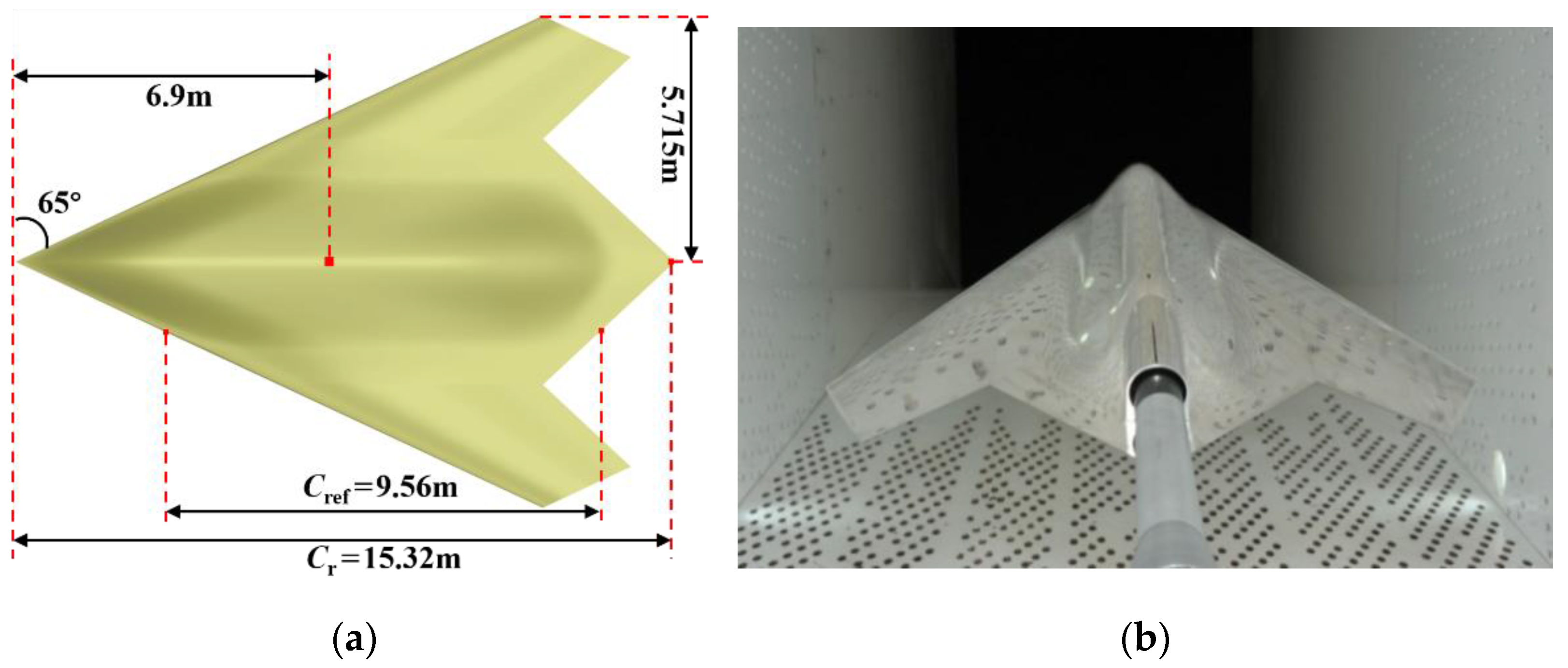
To meet the needs of future aircraft aerodynamic testing and research, relevant domestic institutions are independently designing a blended flying wing common research model for a low-aspect-ratio flying wing shape to use as a general research resource [
3,
4]. The basic geometric parameters of the low-aspect-ratio flying wing model are shown in
Figure 1; the leading-edge sweep back angle is 65°, the rear sweep back angles are 47° and −47°, the length of the whole model is 15.32 m, the averaged aerodynamic chord length is 9.56 m, and the distance between the moment reference point and the leading edge is 6.9 m. For comparison with the experiment results, the model used for simulation and wind tunnel testing is scaled to 1/19.
The reference area of the flying wing model with a small aspect ratio is 0.234 m2, the longitudinal reference length and Reynolds number reference length are the average aerodynamic chord length of 0.5032 m, the reference center of gravity is 45% (non-dimensioned by the fuselage length), and the calculated Mach number and Reynolds number are 0.9 and 10 × 106, respectively. The numerical calculation of the above parameters was consistent with a wind tunnel test carried out.
The test was conducted in a 1.2 m transonic wind tunnel. The size of the transonic test section is 1.2 m (width) × 1.2 m (height) × 3.6 m (length), and the Mach number range is 0.4–3.0, with a control accuracy of 0.005. At Mach 0.9, the corresponding test Reynolds number is 10 × 106, and the flight Reynolds number in the corresponding state is about 80 × 106.
The actual flight Reynolds number is about eight times higher than the test Reynolds number, indicating a certain difference between the generated drag characteristics obtained from the test results and the actual flight. Since the test Reynolds number is one order of magnitude lower than the real flight Reynolds number, the difference in the surface flow state and aerodynamic characteristics of the aircraft caused by the difference in Reynolds number needs further research.
The work presented in this paper accurately evaluated the influence of the Reynolds number and turbulence degree on the aerodynamic characteristics and surface flow state of the small-aspect-ratio flying wing common research model. In this way, the Reynolds number self-calibration area of the small-aspect-ratio flying wing layout studied was determined to be about 10 × 106. It was found to be relatively economical and effective to carry out relevant force measurement tests in a 1.2 m transonic wind tunnel, and aerodynamic characteristics close to the actual flight state could be obtained from the outward differential.
2.2. Calculation Grid
Grid generation technology is the basis of numerical simulation. First, the surface computing grid is generated according to the given digital analog file. To ensure the grid meets the requirements for boundary layer simulation, and so simulates the complex shape of aircraft well, the grid generation idea of “three levels” is adopted. The first level close to the object surface mainly simulates the viscous boundary layer, the second level in the middle mainly simulates the vortex in space, and the third level close to the far field mainly meets the far-field boundary conditions. The block docking grid is adopted based on the shape characteristics of the whole machine. The whole calculation area is divided into several sub-areas surrounded by six curved surfaces. The grid of each sub-area is generated separately, but the grid is completely docked at the connecting surface of each sub-area. Each sub-region grid is generated by the infinite interpolation method and optimized by the elliptic equation. This study adopts the same set of grids each time to reduce the grid correlation of numerical calculation. To meet the requirements of accurate simulation of the turbulent boundary layer, grid generation is carried out based on
M = 0.9 and
y+ ≈ 1 at the flight Reynolds number, and the grid spacing of the first layer in the normal direction is 4.7 × 10
−6 m such that
y+ satisfies o(1) in all states calculated in this study. The growth rate of the normal grid is taken as 1.2.
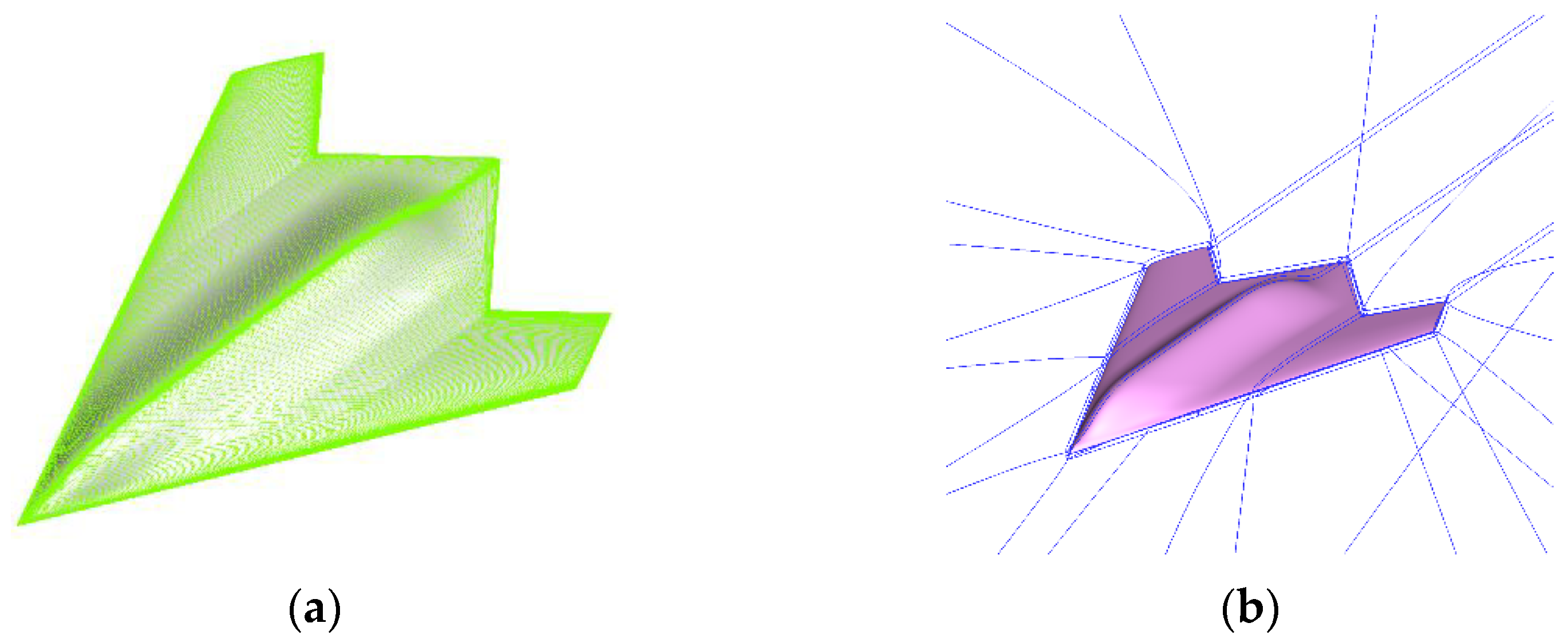
Figure 2 is a schematic of the surface and symmetrical surface grid and topology. The “O” grid topology is adopted, and the size of the calculation area is 50 times that of the average aerodynamic chord length. The number of grids is about 14 million.
Two kinds of boundary conditions are used in this paper. One is the subsonic far-field boundary condition, which is calculated by local one-dimensional Riemann invariants. The solid wall boundary condition without sliding is adopted for the model surface. The pressure is extrapolated from the inner point of the flow field by a zero gradient or constant gradient, and the wall temperature is treated as an adiabatic wall. The model surface temperature is obtained using a one-dimensional energy equation through the relationship between the total and static temperatures. The specific formulas were given in previous work [
3].
The verification of grid independence is added to ensure that the scale and distribution of the numerical grid meet the requirements of accurate prediction of aerodynamic qualities. In combination with the verification of transition prediction methods in
Section 3, the accuracy of the numerical method used in this paper in studying the Reynolds number effect of a small aspect ratio and large swept wing configuration is ensured. The steps are as follows.
The grid refinement factor is defined as
where
N1 and
N2 are the number of grid points in the finer and coarser grids, respectively, and
d is the spatial dimension (3 in our case). The grid convergence index (GCI) is defined as
where
Fs is a safety factor of 3,
p is the order of accuracy for the spatial scheme employed, and
f1 and
f2 are the finer and coarser grid global solution quantities (C
L, C
D, C
m) considered, respectively.
The GCI values for typical aerodynamic coefficients are provided in
Table 1 for α = 2°. The GCI values of the three grids are all relatively low, and they slightly decrease with the increase in grid points. The results indicate that the grid size has little effect on the aerodynamic coefficients of the model, and medium grids can guarantee the simulated reliability.
3. Calibration of Cross-Flow Transition Prediction Method
As the subject is a large swept-angle aircraft, with a leading-edge swept angle of 65°, there is a strong problem of cross-flow transition. To evaluate the Reynolds number’s effect on the transition phenomenon of laminar turbulence more accurately, the parameters of the prediction method are re-calibrated in this section, which improves the accuracy of the transition prediction and the reliability of the calculated results.
Computational fluid dynamics, which use the Reynolds-averaged Navier–Stokes (RANS) to solve equations, have been developed and widely used in engineering. The accurate prediction of the transition position is the key to studying the Reynolds number’s effect. The flying wing layout with a large swept back and small aspect ratio includes an attachment line transition and an unstable TS (Tollmien–Schlichting) wave transition, along with strong cross-flow transition. Accurate simulation poses a considerable challenge to the transition model. This study establishes helicity cross-flow transition correction of the Langtry–Menter model and calibrates the helicity parameters, thus ensuring good prediction accuracy of the cross-flow transition.
The 3D RANS equations are used as the governing equations to describe the physical phenomena, which can be expressed by the finite volume form
where
W is the vector of conservative variables, while
F and
Fv are inviscid and viscous flux vectors, respectively.
is the control volume with the boundary
, and d
S is the infinitesimal face vector.
3.1. Langtry–Menter Transition Prediction Model
The Langtry–Menter transition prediction model consists of two transport equations: the momentum thickness Reynolds number transport Equation (4), and the intermittent factor transport Equation (5):
where
P refers to the production term, and
D refers to the destruction item. The last term at the right end of the two transport equations is the diffusion term, the second term from the left end is the convection term, and
and
are constants representing the calibration parameters of the dissipation term, which are generally obtained based on test results in a large amount of the literature. The suggested values given in the literature are 2.0 and 1.0, respectively. Further to this,
and
are the eddy viscosity coefficients of laminar flow and turbulence, respectively. For the detailed expression of all parameters in Equations (4) and (5), please refer to Langtry’s paper [
22]. To simulate the separated flow, it is necessary to modify solution
to obtain
. In Equation (6),
is constant 2, in which
is the vorticity Reynolds number,
is the critical momentum thickness Reynolds number, and
(
) is the eddy viscosity ratio.
Combining
with the
equation of the SST turbulence model [
21] leads to
In the above equations, and are the source term and failure term of the uncoupled transition prediction model, respectively, and and are the modified source term and failure term, respectively.
3.2. Prediction Model of Cross-Flow Transition Based on Helicity Parameter
This research applies the cross-flow transition prediction model developed by Christoph Muller. The two options to expand Langtry–Menter’s model include changing transport Equation (4) and changing transport Equation (5). The method is based on the cross-flow model selection equation of helicity parameter (2). Expression
of the source term in Equation (4) is as follows:
where
is the constant,
is the momentum thickness Reynolds number based on the incoming flow, and
is the local momentum thickness Reynolds number.
is 1 inside the boundary layer and 0 outside the boundary layer. Finally,
acts inside the boundary layer through diffusion. After considering the influence of cross-flow, the source term of Equation (4) is modified as follows:
is a negative value which provides information about the cross-flow transition. The specific expression is
In the equation,
, where
is the resultant velocity, which maintains the dimensional consistency of Equation (4). In Equation (15) below,
is the momentum thickness of the boundary layer, which can be approximately calculated by
, referring to the Langtry–Menter formula and avoiding the non-local solution.
is the kinematic viscosity coefficient. Equation (15) combines the effects of the
parameters and Reynolds number. The expression
is as follows:
where
is the vorticity, in which
y is the minimum distance from the object surface. The last item
is the parameter used to modify the distance.
are constants, with
being the maximum value of the control cross-flow item generated that does not exceed 0.3 times the original item generated
.
are obtained by comparing the experiment of the NLF (2)—0415 infinite sweep wing. The numerical simulation results are shown below, with the final results being
,
,
,
, and
. There are two reasons why the constant parameters here are different from those in Muller’s article. One is the dimensionless equation, which is mainly due to the change in parameter
. The other reason is that the author recalibrates the parameters according to a comparison of the numerical simulation and the NLF(2)-0415 experiment. Subsequently, the cross-flow model based on the helicity parameter is referred to as the Langtry–Menter–CFH (correction of helicity) model.
After the Reynolds number is calculated as the cross-flow velocity, the source term
, indicating the cross-flow information, can be redefined according to W. Liang’s article [
24] as follows:
In Equation (15), U refers to the local closing speed, the calibration of the six new parameters still adopts NLF0(2)-0415 as the research object, and – are constants (i.e., , , , , , and ). The improved Langtry–Menter–CFH model is called the Langtry–Menter–CFHImproved model.
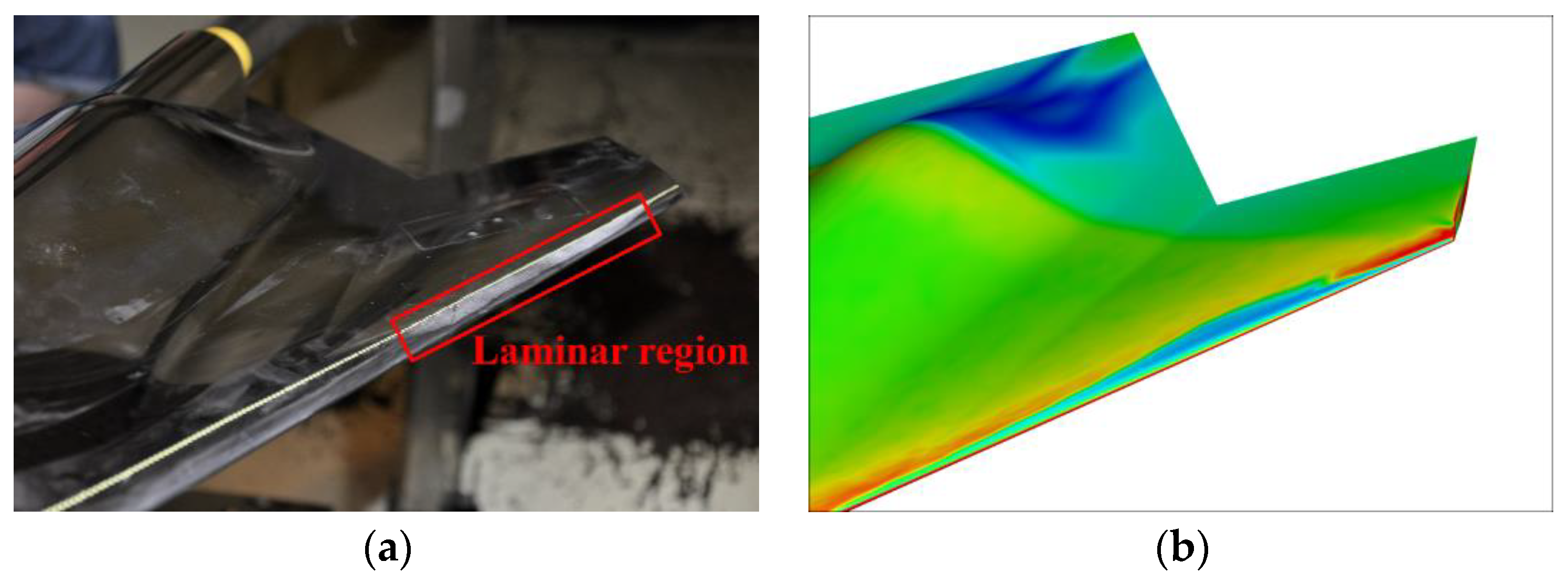
3.3. Example Verification of the DLR-F5 Wing
To verify the robustness of the Langtry–Menter–CFH
Improved model, the DLR-F5 wing is selected as the checking object. The leading-edge sweep angle of the wing is 20°, a supercritical symmetrical airfoil is adopted, the Mach number is 0.82, the model angle of attack is 2°, the reference chord length is 0.15 m, the reference area is 0.16 m
2, and the Reynolds number is 1.5 × 10
6. The wind tunnel experiment was developed by Sobieczky (1994). In the wind tunnel, the wing is directly installed on the side wall of the test section. The first layer of the computational grid boundary layer ensures that
y+ is less than 1, the growth rate is 1.15, and the number of grids is six million. In this study, the Langtry–Menter model and Langtry–Menter–CFH
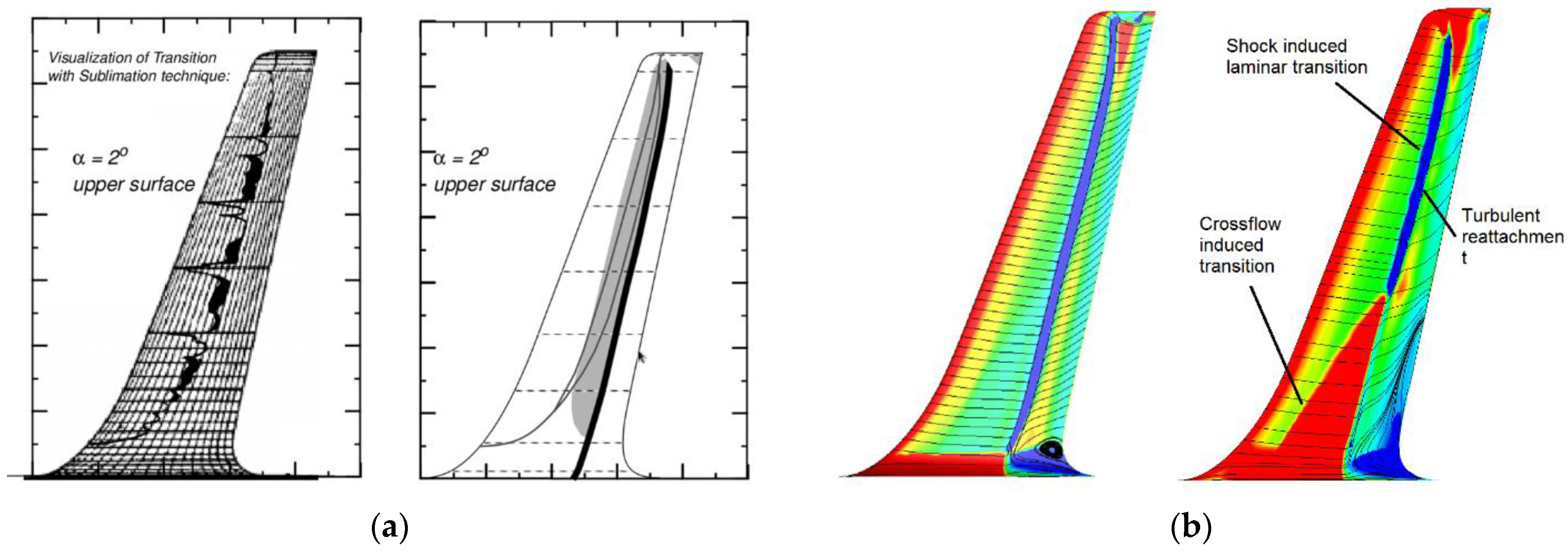
Improved model were used for numerical simulations. The experimental results and numerical simulation results are shown in
Figure 3. The two gray lines along the flow direction in the right panel of
Figure 3a are the beginning and end of the transition, respectively; the gray area is the mixed area of transition and separation; the black thick line is the shock compression area.
Figure 3b shows that from the numerical simulation results, the Langtry–Menter–CFH
Improved model can capture the cross-flow transition phenomenon at the wing root of DLR-F5, but the Langtry–Menter model does not have this ability.
5. Conclusions
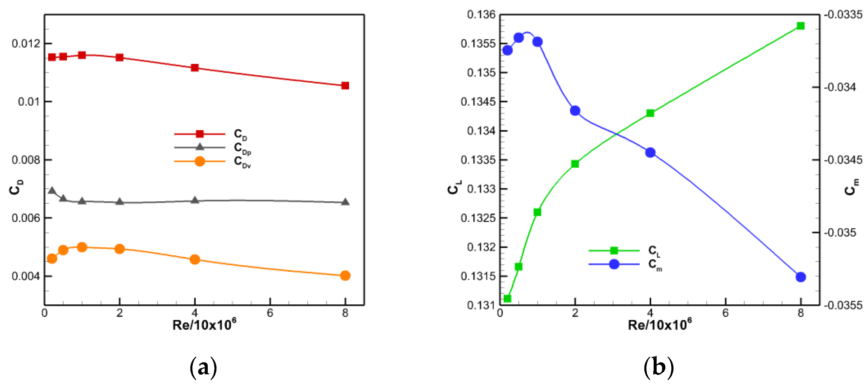
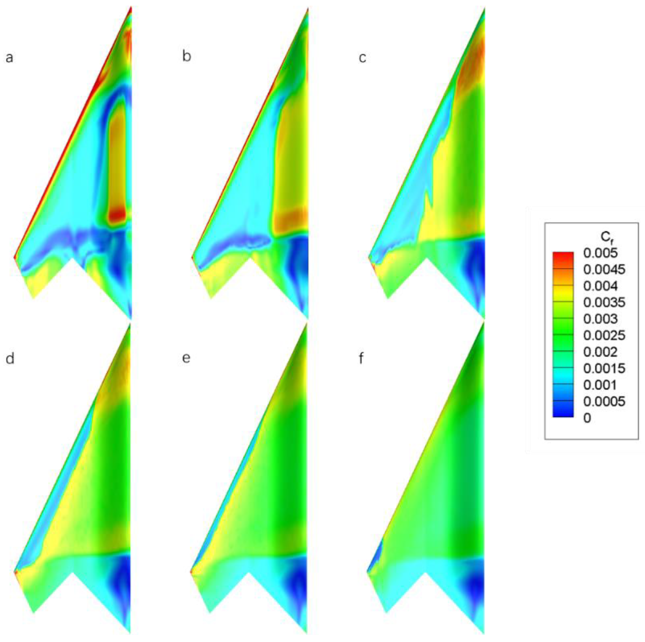
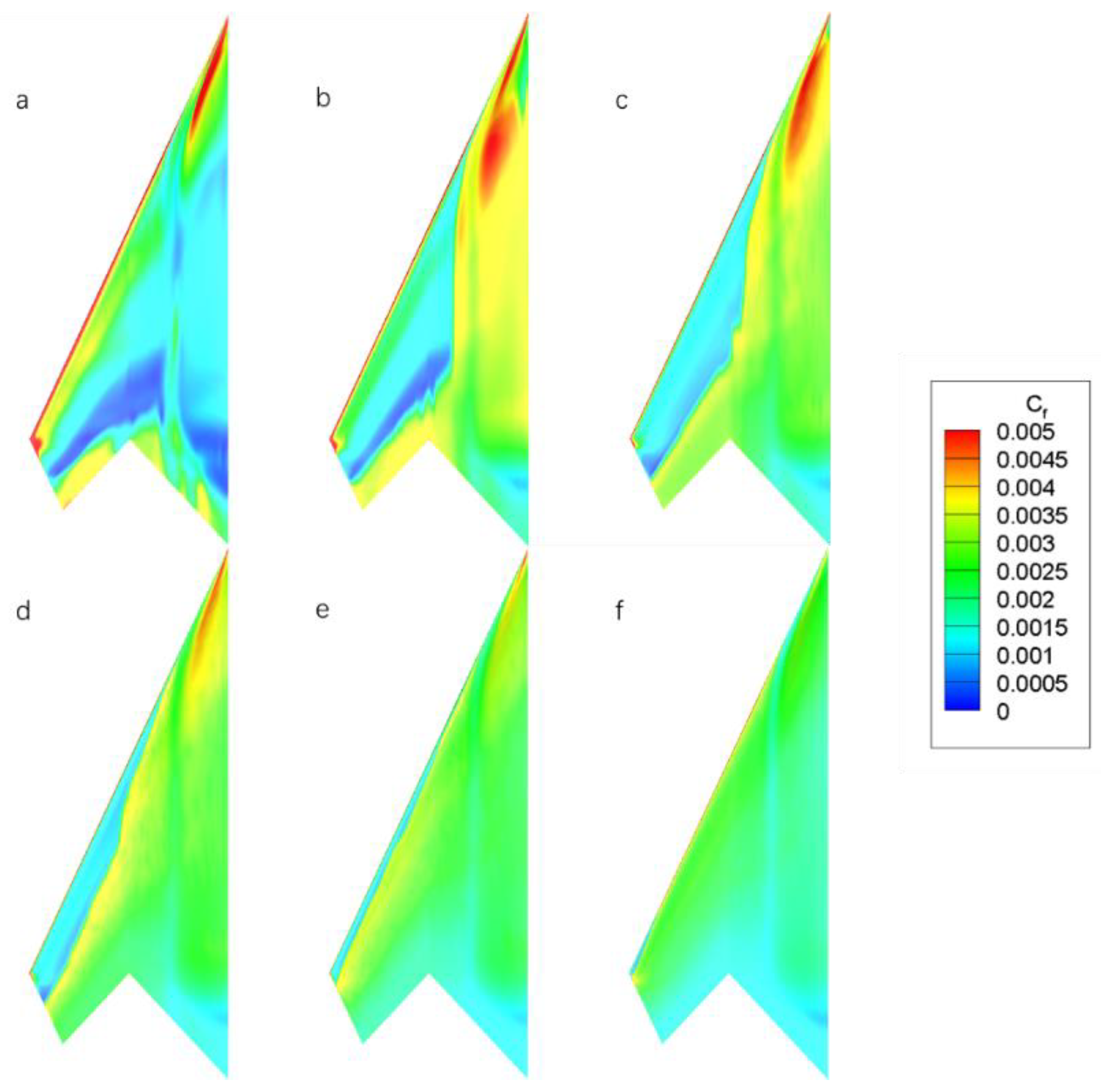
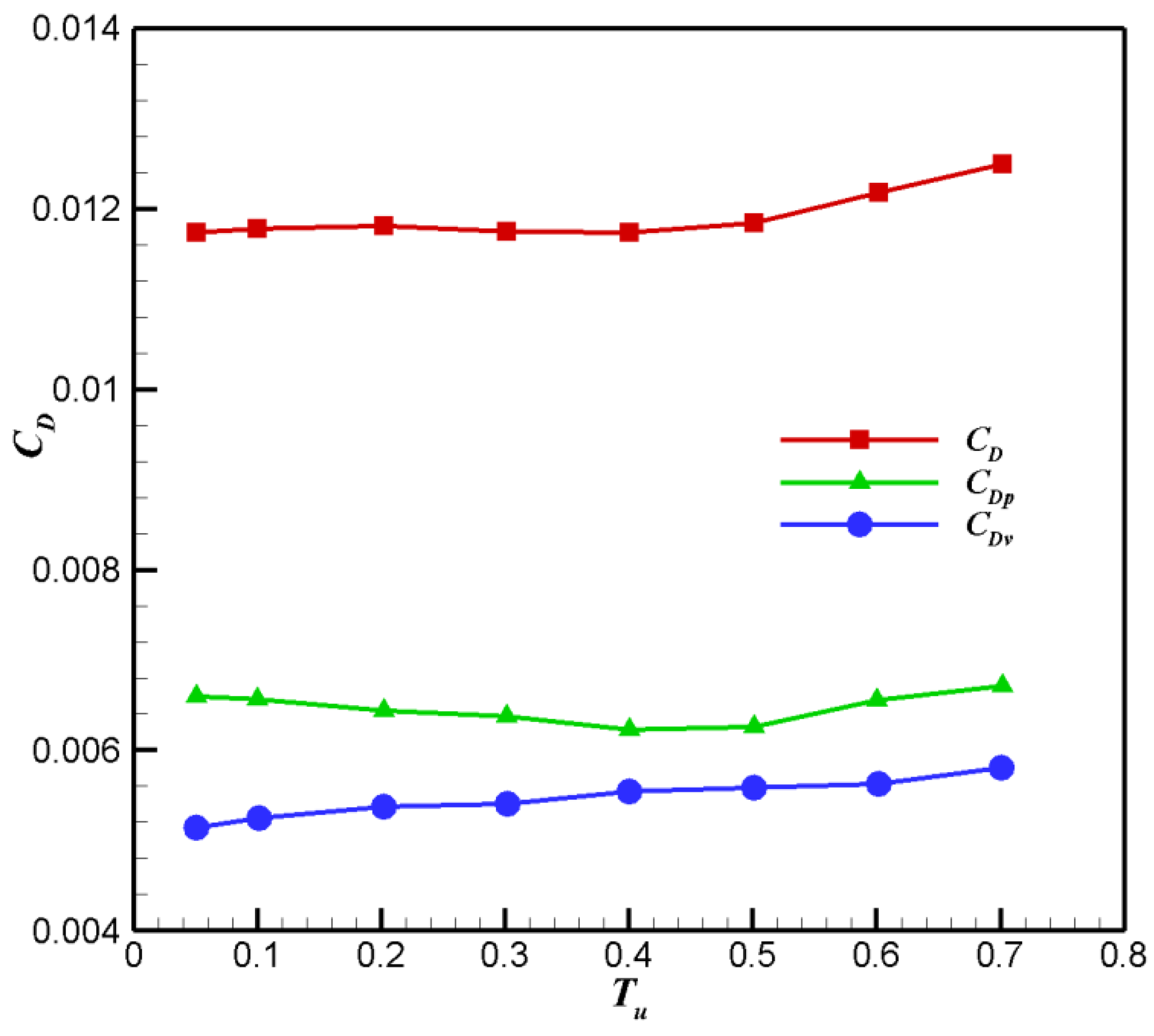
This study established the helicity cross-flow transition correction of the Langtry–Menter model and calibrated the helicity parameters, generating good prediction accuracy for the cross-flow transition. In the case of a small angle of attack, the Reynolds number mainly affects the size of the friction. With an increase in the Reynolds number, the laminar flow range decreases, and the turbulent viscosity increases. Under this comprehensive effect, the friction resistance coefficient first increases and then decreases, reaching a maximum when the Reynolds number is about 10 × 106 but having little effect on the pressure drag. The influence of turbulence intensity on the aerodynamic characteristics of a small-aspect-ratio layout is relatively small. When the turbulence intensity is greater than 0.4%, this reduces the surface laminar flow range and increases the drag coefficient. The test Reynolds number is close to the self-aligning Reynolds number of the flying wing standard model with a small aspect ratio. Therefore, the aerodynamic characteristics under the test Reynolds number are very close to the flight Reynolds number. When extrapolating the wind tunnel test results, only the drag coefficient needs to be corrected.
The effects of the Reynolds number and turbulence on the aerodynamic characteristics and boundary layer state of aircraft with a flying wing with a small aspect ratio were accurately evaluated, and the Reynolds number self-simulation region of the small-aspect-ratio flying wing configuration was about 10 × 106. Based on the results, it is clear that it is relatively economical and effective to conduct force measurement tests in a 1.2 m transonic wind tunnel. The aerodynamic characteristics of the actual flight state can be determined through modified extrapolation.
The current research focus is on the cruise status of a low-aspect-ratio flying wing configuration. In the future, we will focus on the secondary separation of the leeward and shock-induced vortex breakdown characteristics with Reynolds-number effects for a low-aspect-ratio flying wing configuration at a high angle of attack.


 ,
, 


