
Assessment of Potential Conflict Detection by the ATCo

 ,
,  ,
,  , , and
Abstract
:1. Introduction
1.1. Principles of Bayesian Network Analysis
- -
- G is a directed acyclic graph in which each node represents one of the variables X1, X2, …, Xn, and each arc represents direct dependence relationships between the variables. The direction of the arcs indicates that the variable “pointed to” by the arc depends on the variable at its origin.
- -
- T is a set of parameters that quantify the network. It contains the probabilities PB(xi|pxi) for each possible value xi of each variable Xi and each possible value pxi of PXi, where the latter denotes the set of parents of Xi in G. Thus, a Bayesian network B defines a unique joint probability distribution over U.
The Main Reasons for Selecting Bayesian Network Methods
- -
- Bayesian networks are very useful for capturing and analysing causality and influence relationships. They are very effective for diffusing uncertainty and updating systems with new data. They are also applicable when the structure of the system is too complex. They provide an intuitive and efficient way to represent a large field, making it feasible to model complex systems.
- -
- Bayesian networks are primarily used to update the probability distribution of the states of hypothetical variables (variables that cannot be directly observed). This probability distribution helps decision-makers determine the appropriate course of action.
- -
- Bayesian networks provide a convenient and consistent way of expressing uncertainty in uncertainty models and are increasingly used to express knowledge. They are used for qualitative and quantitative modelling of uncertainty and its causes.
- -
- Due to the conditional dependence of the variables in the network, BNs provide the ability to predict or diagnose (i.e., they can determine impact and causes). BNs are used to model multidirectional forward and backward uncertainties.
- -
- Qualitative analysis: Given a scene, the BN graphically represents the causal relationship between the different elements of the scene.
- -
- Quantitative analysis: Updating the probability distribution. Given the hypothetical variables representing the possible actions and the prior probability distribution, the BN provides the function of updating this probability distribution when new data and information are acquired.
2. Methodology
- -
- Development of the Bayesian Network Model (BNM). The development of the BNM starts with a characterisation of the safety event in terms of safety dimensions (precursors) and their aggregation. The result of this descriptive analysis, together with prior statistical knowledge, serves to structure the model that could provide statistical representations of the frequency and severity of the safety event.
- -
- Calibration, tuning and sensitivity analysis of the Bayesian Network Model (BNM). The model proposed in the previous task is fitted and calibrated on real data. The explanatory power of the model and/or of each independent variable and mixed effects is quantified. The sensitivity analysis considering mixed effects allows characterising the safety performance in terms of not only the independent dimensions, but also of their combinations, identifying the prior thresholds of these dimensions that would reduce the frequency of a safety event.
- -
- Most influential factors in the Bayesian Network Model (BNM). Application of the model to the defined case study or scenario to quantify the most influential factors.
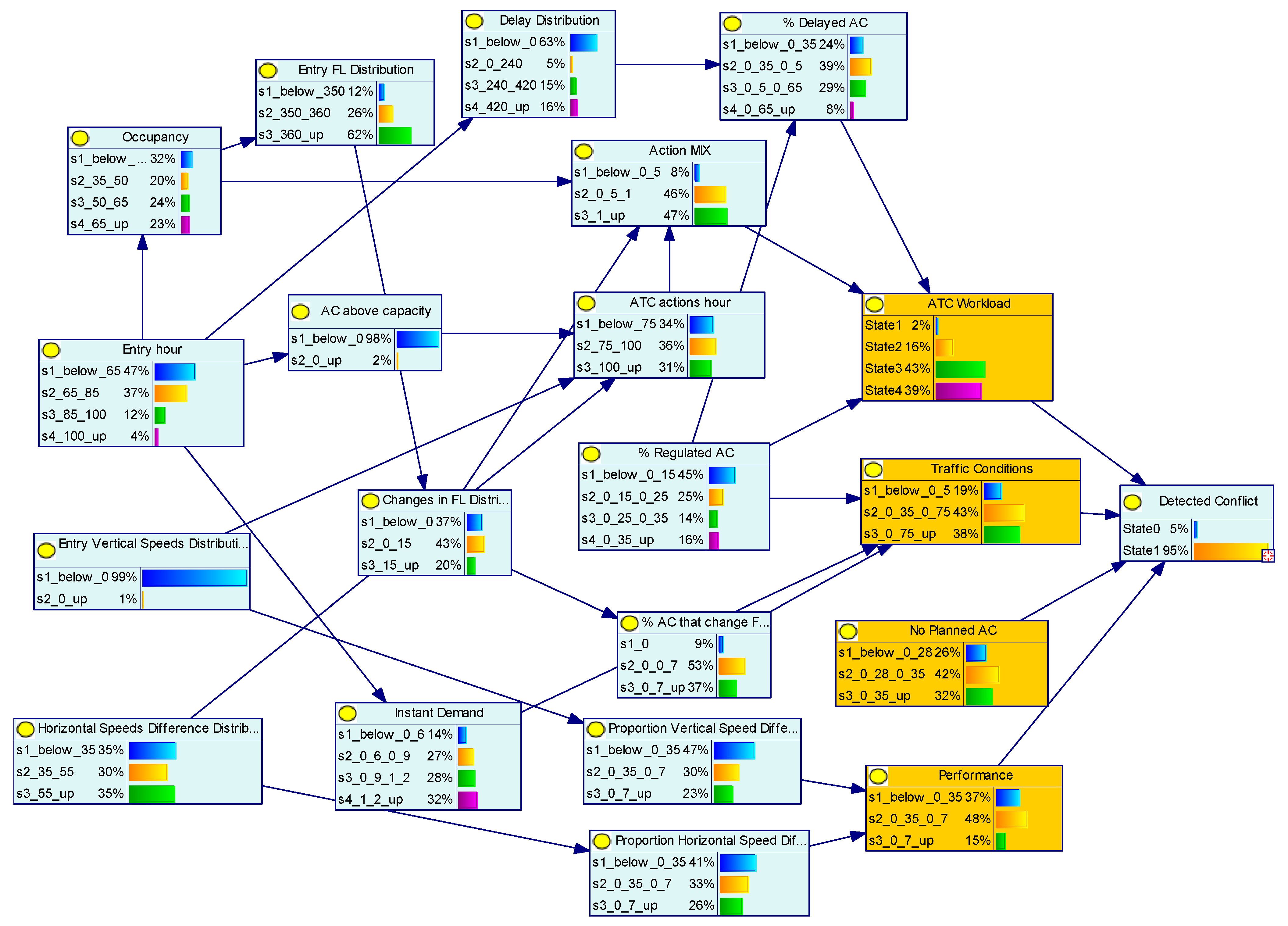
3. Development of the Bayesian Network Model (BNM)
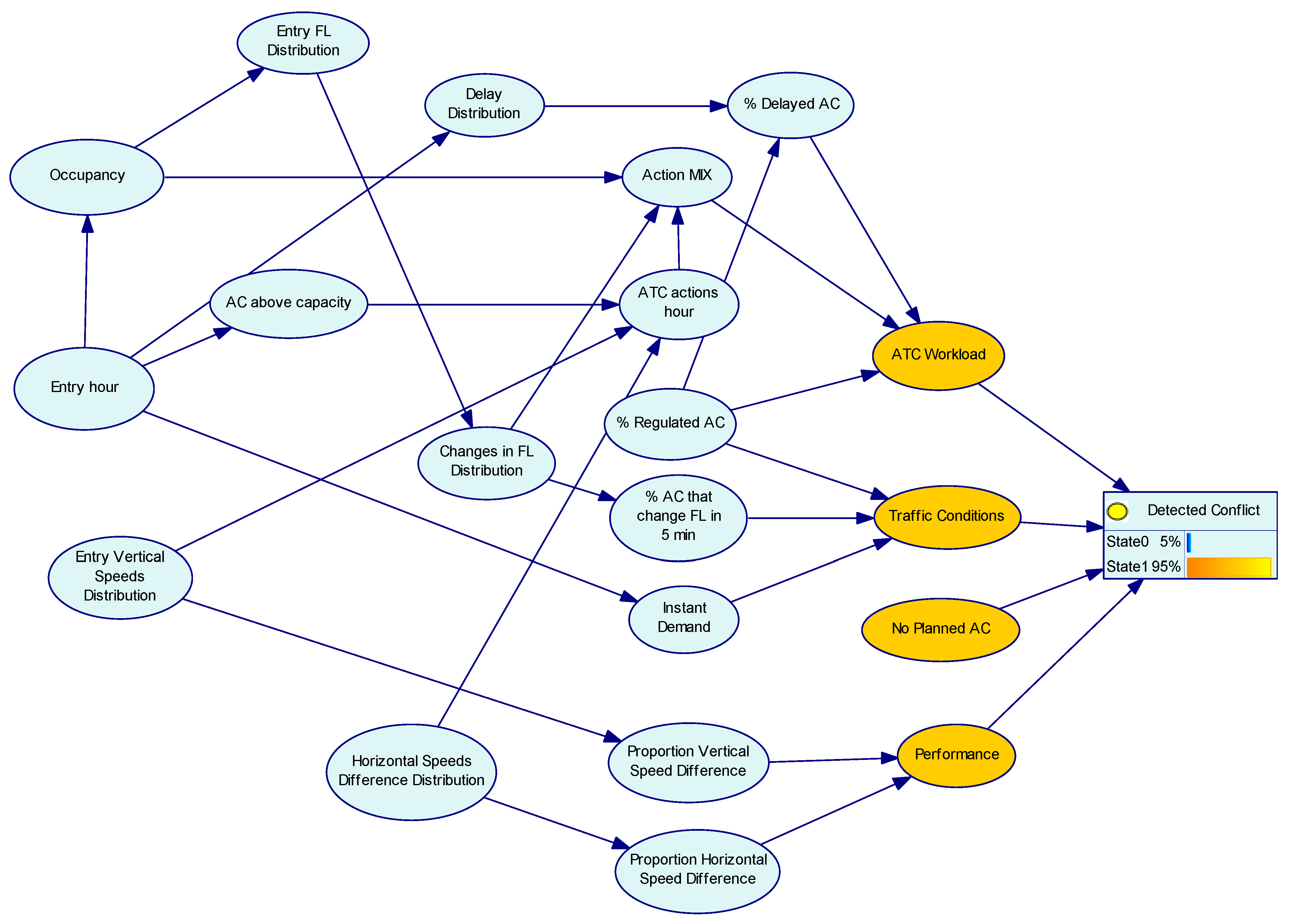
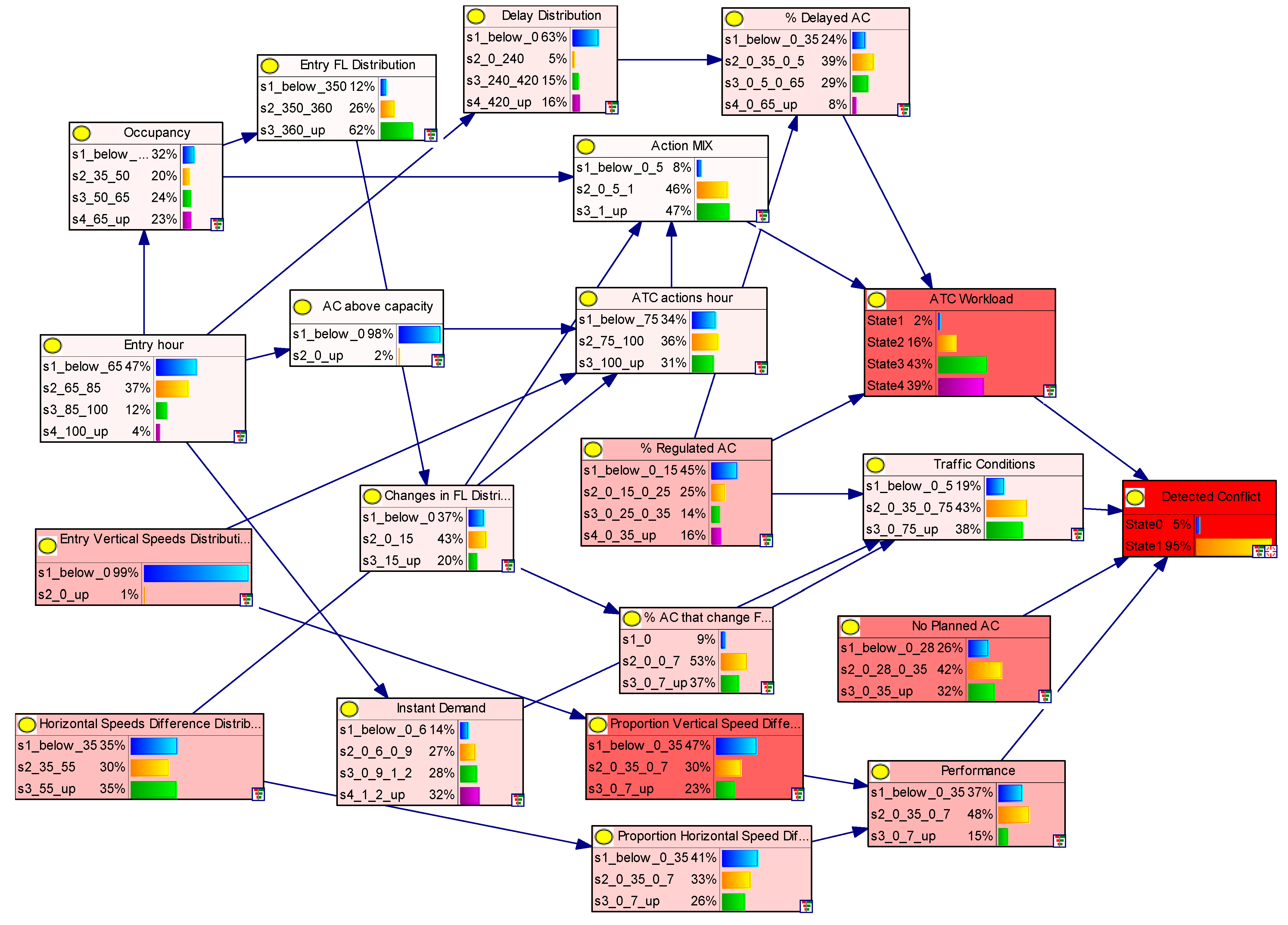
3.1. Construction of the BN
- o
- Traffic conditions.
- o
- Aircraft performance.
- o
- Not expected aircraft in the sector.
- -
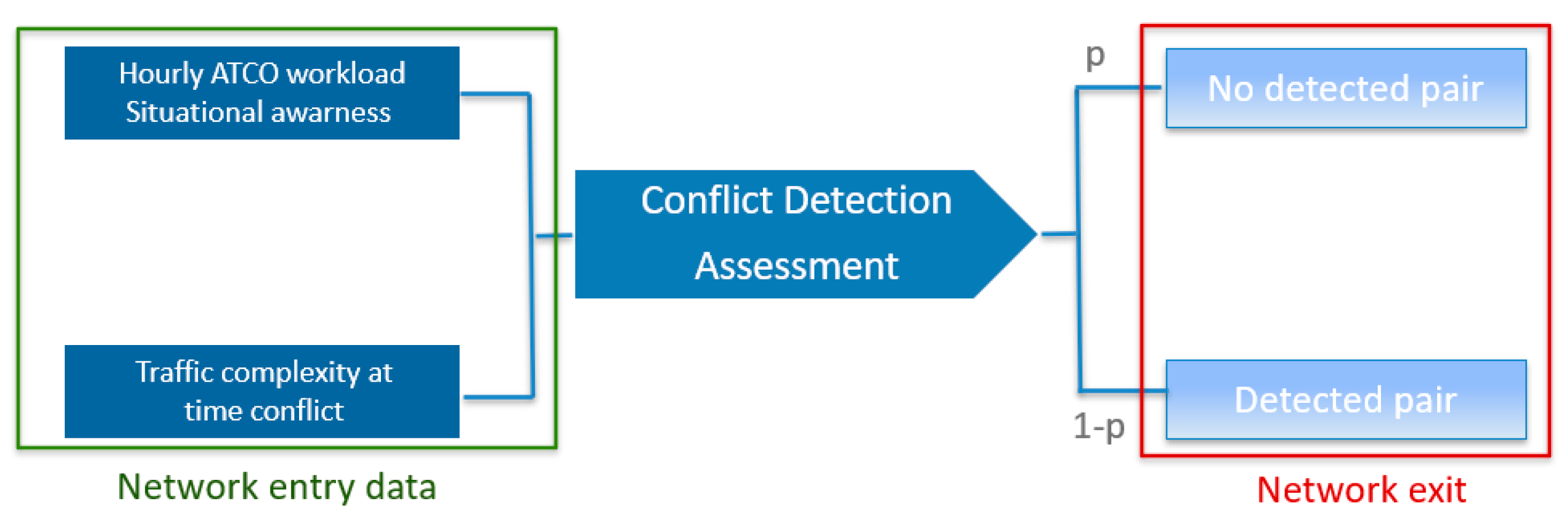
- Network entry: It shall consist of the four inputs already mentioned, composed of the ATCo workload plus the three variables characterising the complexity of the scenario (traffic conditions, aircraft performance and unexpected aircraft).
- -
- Training data: The network is trained with the conditions of each record.
- -
- Network exit: The output will be the probability that the ATCo detects the potential conflict. Note that the conflict will be considered detected whenever the air traffic controller takes any action on any of the two aircraft involved.
3.1.1. ATCo Alert Status Analysis Area
- -
- Network entry: Global parameters of the hour, referring to traffic density and ATCo actions during the hour.
- -
- Training data: Considering the sector conditions, it is trained to identify the ATCo actions in the hour, and in particular the authorisations to resolve a conflict (flight level change, direct to, reroute).
- -
- Network exit: The workload level, defined in four states:
- o
- Level 1: Number of high-resolution actions, and high total number of actions.
- o
- Level 2: Number of medium resolution actions, and total number of actions high.
- o
- Level 3: Number of medium resolution actions and medium total number of actions.
- o
- Level 4: Low number of total actions.
3.1.2. Scenario Conditions Analysis Area
- -
- Network entry: Average of the scenario parameters in the 5 min period identified in time.
- -
- Parameter calculation: Considering the scenario conditions, training is carried out to evaluate the three parameters that characterise the scenario and which are described below:
- o
- Traffic conditions: defined by parameters such as instantaneous demand (count of number of aircraft entering the sector), the percentage of regulated aircraft and the distribution of flight levels. All these variables are evaluated at 5 min time intervals.
- o
- Aircraft performance: Defined by vertical and horizontal speed distributions.
- o
- Unexpected aircraft in the sector: Both out-of-flow and unexpected aircraft are considered; however, as it was not possible to obtain data related to these flows, only the first variable will be used.
- -
- Instantaneous demand: Ratio of instantaneous demand to average maximum instantaneous demand on the day in question (maximum shall be 1).
- -
- % Regulated aircraft: % of regulated aircraft with respect to the total in the period of time in question on a scale of 0–1. The fact that the aircraft are regulated means that the flow will be continuous.
- -
- % Aircraft changing FL in the period: % of aircraft changing FL relative to the total in the time period in question on a scale of 0–1.
- -
- Speed distribution: Complexity occurs when aircraft have differences in speed. Therefore, the speed difference between the two aircraft is compared:
- o
- % Aircraft with a speed difference greater than 50 knots: % on a scale of 0 to 1.
- o
- Vertical speed distribution: Complexity occurs when ACs climb or descend with different speeds. Therefore, the difference in speeds between the two aircraft is compared.
- o
- % of AC with non-zero vertical speed difference: % on a scale of 0–1.
- o
- % Unexpected AC: % of aircraft that have changed EOBT time against IOBT.
4. Calibration, Fitting and Sensitivity Analysis of the Bayesian Network Model (BNM)
4.1. Parametric Learning
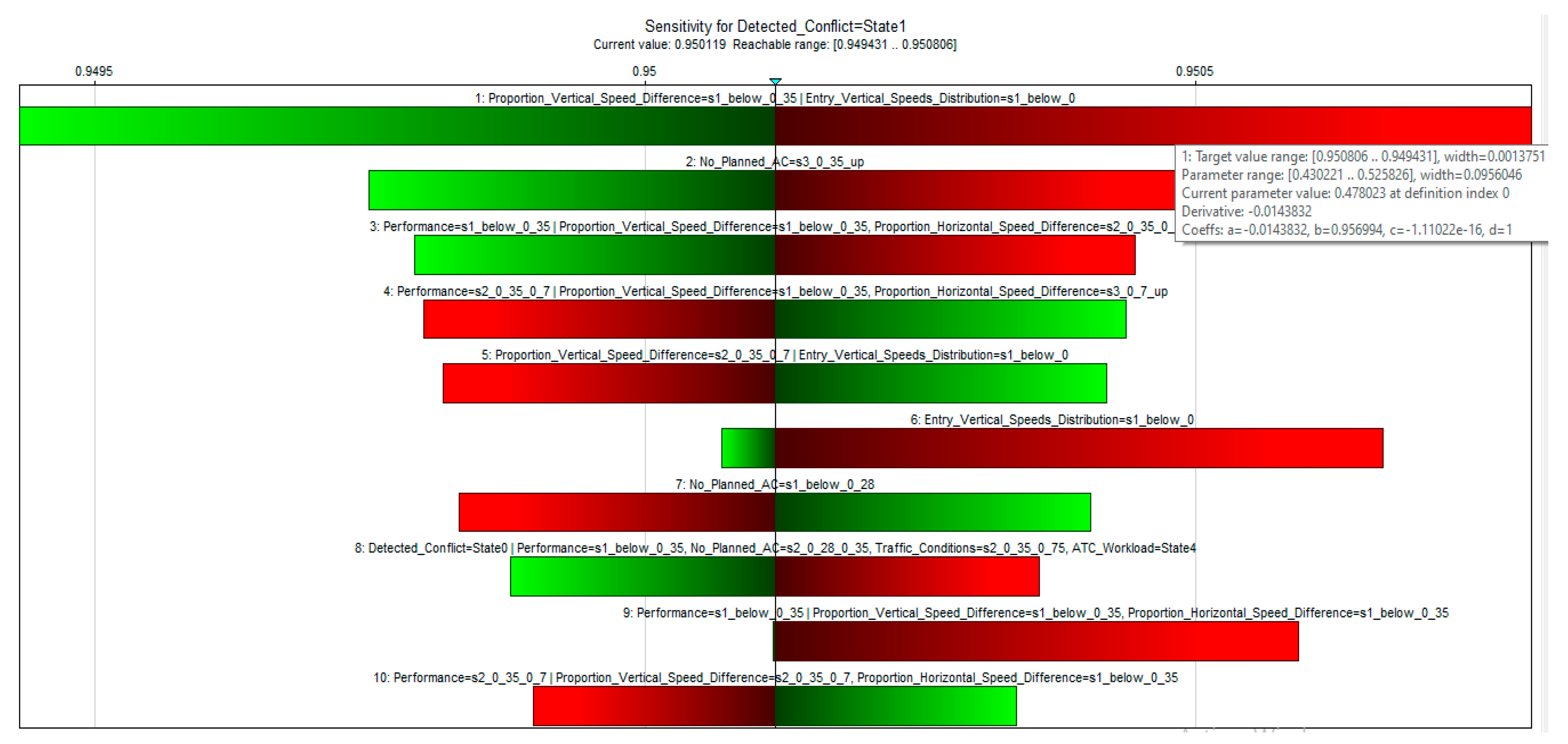
4.2. Sensitivity Analysis
5. Discussion: Most Influential Factors in the Bayesian Network Model (BNM)
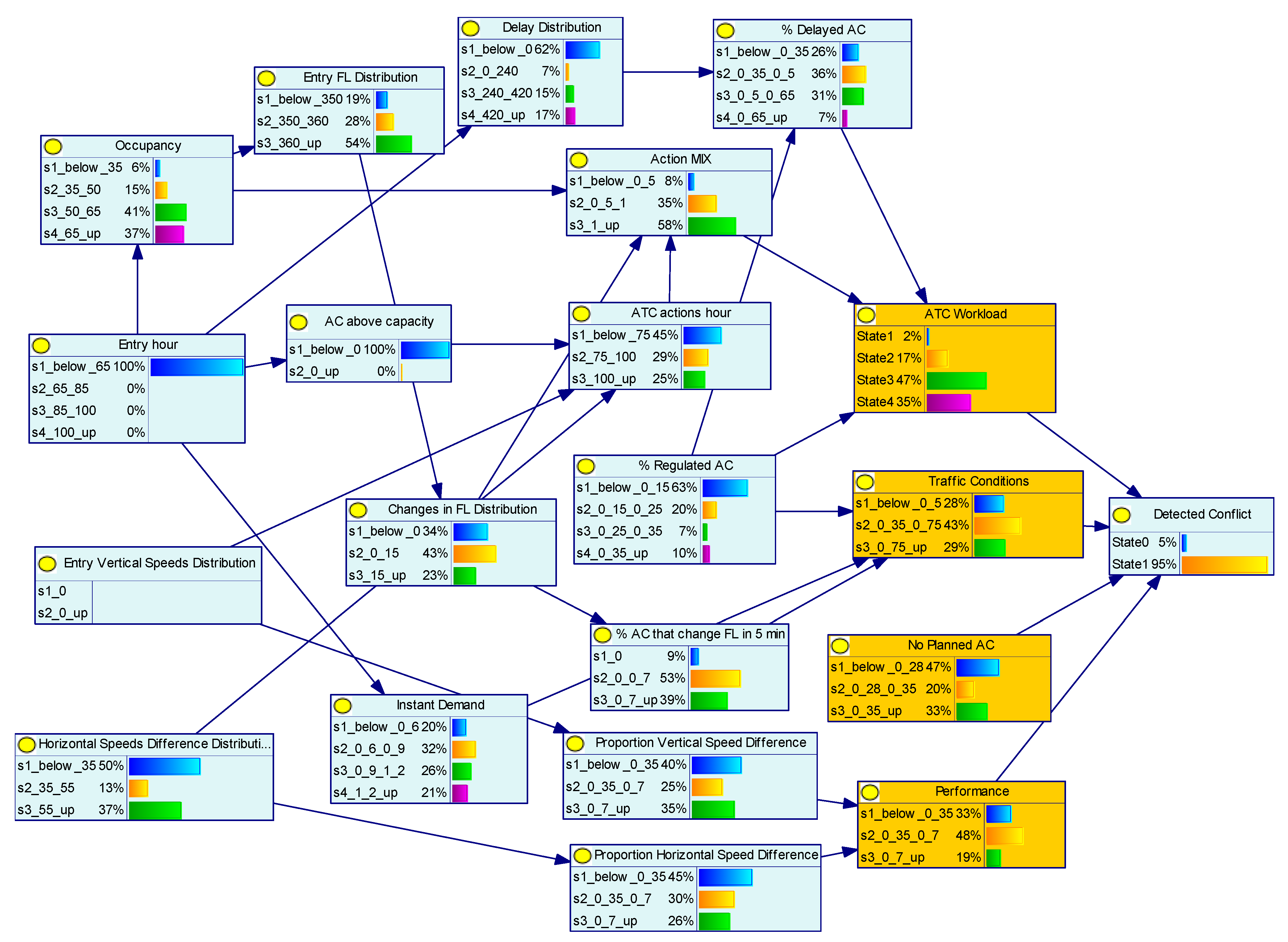
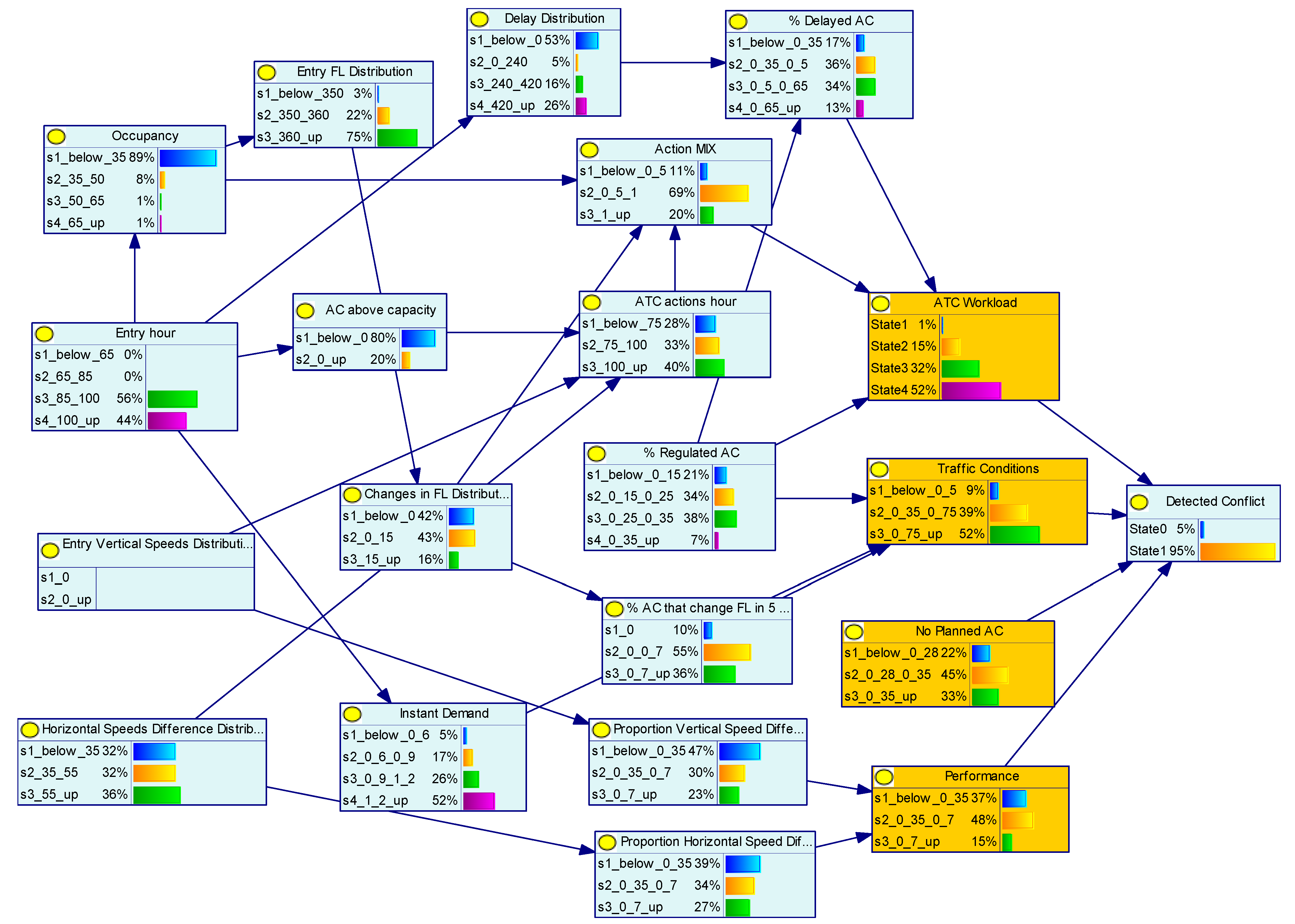
Forward Analysis
6. Validation
7. Conclusions
Author Contributions
Funding
Institutional Review Board Statement
Informed Consent Statement
Data Availability Statement
Conflicts of Interest
References
- FARO Consortium. D2.1 Project Scope. SESAR 3 Joint Undertaking under the European Union’s Horizon 2020. Available online: https://faro-h2020.eu/downloads/ (accessed on 20 July 2022).
- Eurocontrol. ESARR Advisory Material/Guidance Document (EAM/GUI) EAM 2/GUI 8; Eurocontrol: Brussels, Belgium, 2005. [Google Scholar]
- Valdés, R.A.; Comendador, F.G. New European Union Approach to Civil Aviation Accident Investigation and Prevention. J. Aircr. 2011, 48, 1396–1404. [Google Scholar] [CrossRef]
- Kuchar, J.; Yang, L. A review of conflict detection and resolution modeling methods. IEEE Trans. Intell. Transp. Syst. 2000, 1, 179–189. [Google Scholar] [CrossRef]
- SESAR Joint Undertaking. SESAR 2020 Safety Reference Material, Brussels, Belgium. 2018. Available online: https://www.sesarju.eu/sites/default/files/documents/transversal/SESAR2020%20Safety%20Reference%20Material%20Ed%2000_04_01_1%20(1_0).pdf (accessed on 20 July 2022).
- Nazeri, Z.; Barbara, D.; Jong, K.D.; Donohue, G.; Sherry, L. Contrast-Set Mining of Aircraft. In Proceedings of the Industrial Conference on Data Mining, Leipzig, Germany, 16–18 July 2008; Springer: Berlin/Heidelberg, Germany, 2008; pp. 313–322. [Google Scholar]
- Oztekin, A. A Data-Driven Quantitative Framework for Safety Assessment of Air Traffic Control System. In Proceedings of the 15th AIAA Aviation Technology, Integration, and Operations Conference, Dallas, TX, USA, 22–26 June 2015. [Google Scholar] [CrossRef]
- Verstraeten, J.; van Baren, G.B.; Wever, R. The Risk Observatory: Developing an Aviation Safety. J. Saf. Stud. 2016, 2, 91. [Google Scholar] [CrossRef]
- Ayra, E.S.; Ríos Insua, D.; Cano, J. Bayesian Network for Managing Runway Overruns. J. Aerosp. Inf. Syst. 2019, 16, 546–558. [Google Scholar]
- Miaou, S.P.; Lord, D. Modeling traffic crash-flow relationships for intersections: Dispersion. J. Transp. Res. 2003, 1840, 31–40. [Google Scholar]
- Valdés, R.M.A.; Comendador, V.F.G.; Sanz, L.P.; Sanz, A.R. Prediction of aircraft safety incidents using Bayesian inference and hierarchical structures. Saf. Sci. 2018, 104, 216–230. [Google Scholar] [CrossRef]
- Hauer, E.; Harwood, D.W.; Council, F.M.; Griffith, M.S. Estimating Safety by the Empirical Bayes Method: A Tutorial. Transp. Res. Rec. J. Transp. Res. Board 2002, 1784, 126–131. [Google Scholar] [CrossRef]
- Valdés, R.A.; Comendador, V.F.G.; Castan, J.A.P.; Sanz, A.R.; Sanz, L.P.; Nieto, F.J.S.; Aira, E.S. Bayesian inference in Safety Compliance Assessment under. Saf. Sci. 2019, 116, 188–195. [Google Scholar]
- Heydari, S.; Miranda-Moreno, L.F.; Lord, D.; Fu, L. Bayesian Methodology to Estimate and Update SPF Parameters under Limited Data Conditions: A Sensitivity Analysis. Accid. Anal. Prev. 2014. [Google Scholar] [CrossRef] [PubMed]
- Acarbay, C.; Kiyak, E. Risk mitigation in unstabilized approach with fuzzy Bayesian bow-tie analysis. Aircr. Eng. Aerosp. Technol. 2020, 92, 1513–1521. [Google Scholar] [CrossRef]
- Bujor, A.; Ranieri, A. Assessing Air Traffic Management Performance Interdependencies through Bayesian Networks: Preliminary Applications and Results. J. Traffic Transp. Eng. 2016, 4, 34–48. [Google Scholar] [CrossRef]
- Comendador, V.F.G.; Valdés, R.M.A.; Diaz, M.V.; Parla, E.P.; Zheng, D. Bayesian Network Modelling of ATC Complexity Metrics for Future SESAR Demand and Capacity Balance Solutions. Entropy 2019, 21, 379. [Google Scholar] [CrossRef] [PubMed] [Green Version]
- CANSO. Incidents Investigation Toolbox. 2021. Available online: https://canso.fra1.digitaloceanspaces.com/uploads/2021/04/CANSO-Incidents-Investigation-Toolbox.pdf (accessed on 10 February 2022).
- Santiesteban Rojas, J.C.; Utria Pérez, D.; Hernández Reyes, C.E. Definition of Bayesian Networks and their applications. Vinculando J. 2012. Available online: https://www.bu.edu/sph/files/2014/05/bayesian-networks-final.pdf (accessed on 20 July 2022).
- Netjasov, F.; Crnogorac, D.; Pavlović, G. Potential safety occurrences as indicators of air traffic management safety performance: A network based simulation model. Transp. Res. Part C Emerg. Technol. 2019, 102, 490–508. [Google Scholar] [CrossRef]
- ICAO. Application of Separation Minima; ICAO: Montreal, QC, Canada, 2020. [Google Scholar]
- FARO Consortium. D4.1 Safety Performance Functions Methodology. 2021. Available online: https://faro-h2020.eu/wp-content/uploads/2021/12/D41-Safety_Performance_Functions_Methodology_v00.01.01_Public.pdf (accessed on 20 July 2022).
- Jurado, R.D.A.; Comendador, V.F.G.; Suárez, M.Z.; Moreno, F.P.; Gallego, C.E.V.; Valdes, R.M.A. Safety performance functions to predict separation minima infringements in en-route airspace. In Aircraft Engineering and Aerospace Technology; Emerald Publishing Limited: Bingley, England, 2022; p. 10. ISSN 1748-8842. [Google Scholar] [CrossRef]
- FARO Consortium. D6.2—Validation Report. SESAR 3 Joint Undertaking under the European Union’s Horizon 2020. Available online: https://faro-h2020.eu/downloads/ (accessed on 20 July 2022).
- Buselli, I.; Oneto, L.; Dambra, C.; Gallego, C.V.; Martınez, M.G.; Smoker, A.; Ike, N.; Martino, P.R.; Pejovic, T. Natural Language Processing and Data-Driven Methods for Aviation Safety and Resilience: From Extant Knowledge to Potential Precursors. In Proceedings of the 11th SESAR Innovation Days, Virtual, 7–9 December 2021. [Google Scholar]
- Sensitivity Analysis in Bayesian Networks (and Influence Diagrams). 2016. Available online: https://support.bayesfusion.com/docs/GeNIe/bn_sensitivitybn.html (accessed on 15 December 2021).
- Borgonovo, E. Sensitivity Analysis: An Introduction for the Management Scientist; International Series in Operations Research & Management Science; Springer: New York, NY, USA, 2019. [Google Scholar]
- Pejovic, T.; Netjasov, F.; Crnogorac, D. Relationship between Air Traffic Demand, Safety and Complexity in High-Density Airspace in Europe. In Risk Assessment in Air Traffic Management; IntechOpen: London, UK, 2020. [Google Scholar] [CrossRef] [Green Version]


| Parameter | Description | Discretisation Criteria | Discretisation Example |
|---|---|---|---|
| Occupancy | Occupation Sector data at the AC entry hour | It is divided into 4 intervals that represent the percentage of occupation in the sector at the AC entry hour respect to the maximum value detected in the sector. The values of the intervals depend on the sector data. | Value < 40% 40% < value < 65% 65% < value < 85% 85% < value |
| Entry | Entries Sector data at the AC entry hour | It is divided into 4 intervals that represent the percentage of entries in the sector respect to the sector entry declared value at the AC entry hour. The values of the intervals depend on the sector data. | Value < 55% 55% < value < 65% 65% < value < 80% 80% < value |
| Instant demand | Ac entry data in the sector in the 5 min period | It is divided into 4 intervals that represent the percentage respect to the maximum instantaneous demand value. The values of the intervals depend on the sector data. | Value < 60% 60% < value < 90% 90% < value < 120% 120% < value |
| AC above capacity | Percentage of aircraft exceeding declared capacity per hour | It is divided into two states, when the percentage of AC above capacity is equal to 0 and when it is greater than 0 | Value = 0 Value > 0 |
| Entry FL Distribution | Calculation of the median flight level with which AC enter the sector at the entry hour | It is divided into three intervals that represent the entry FL distribution in the sector | Value < 350 350 < Value < 360 Value > 360 |
| Horizontal Speeds Differences Distribution | Calculation of the median horizontal speeds with which AC enter the sector at the entry hour | It is divided into three intervals that represent the entry Horizontal Speed Difference Distribution in the sector | Value < 35 35 < Value < 55 Value > 55 |
| Entry Vertical Speeds Distribution | Calculation of the median vertical speeds with which AC enter the sector at the entry hour. It is calculated in absolute value | It is divided into two states, when the median of entry Vertical speed is 0 and when it is greater than 0. This discretisation is intended to represent the complexity for the controller, modelling the AC that are ascending or descending. | Value = 0 Value > 0 |
| Changes in FL distribution | Calculation of the median percentage of AC that change their FL in the sector at the entry hour | It is divided into three intervals, that depends on the sector data. | Value = 0 0% < Value < 15% Value > 15% |
| Delay Distribution | Calculation of the median time delayed of AC at the entry hour into the sector | It is divided into four intervals that represent the delay time (seconds) in the sector. These intervals depend on the sector data | Value = 0 0 < Value < 240 240 < Value < 420 420 < Value |
| % Regulated AC | Calculation of the percentage of AC that have some regulation at the entry hour | It is divided into four intervals. These intervals depend on the sector data | Value < 15% 15% < Value < 25% 25% < Value < 35% 35% < Value |
| % Delayed AC | Calculation of the percentage of AC that have some delay at the entry hour | It is divided into four intervals. These intervals depend on the sector data | Value < 35% 35% < Value < 50% 50% < Value < 65% 65% < Value |
| ATCo actions hour | Calculation of the total actions that the controller has given in one hour in the sector | It is divided into three intervals, which are intended to represent the workload of ATCo according to the action they have undertaken. These intervals depend on the sector data | Value < 75 75 < Value < 100 Value > 100 |
| Action MIX | Sum of resolution actions of any kind. This variable considers flight level changes, vectors and directs. | Resolution actions are added, and the same three categories are defined | Value < 0.5 0.5 < Value < 1 Value > 1 |
| % AC that change FL in 5 min | Distribution of aircraft by number of flight levels that change | It is divided into three intervals | Value = 0% 0% < Value < 70% 70% < Value |
| Proportion Vertical Speed Difference | Calculation of the percentage of AC with vertical speed difference other than 0, on a scale of 0–1 | It is divided into three intervals that represent the complexity when ACs are ascending or descending with different speeds. | Value < 0.35 0.35 < Value < 0.7 0.7 < Value |
| Proportion Horizontal Speed Difference | Calculation of the percentage of AC with horizontal speed difference greater than 50 knots: on a scale of 0–1 | It is divided into three intervals that represent the complexity when ACs have speed difference | Value < 0.35 0.35 < Value < 0.7 0.7 < Value |
| ATC Workload | Combination of total actions with resolution actions | This output node is divided into four states, as defined in the first sections | Level 1 Level 2 Level 3 Level 4 |
| Traffic Conditions | Relative situation of each aircraft pair | This output node is divided into three states, in order to model the traffic conditions at the conflict moment | Value < 0.5 0.5 < Value < 0.75 0.75 < Value |
| No Planned AC | Unexpected aircraft or aircraft operating outside standard flows in the 5 min period | This output node is divided into three states from 0 to 1 | Value < 0.28 0.28 < Value < 0.35 0.35 < Value |
| Performance | Considers the difference in aircraft performances at time t | This output node is divided into three states from 0 to 1 | Value < 0.35 0.35 < Value < 0.7 0.7 < Value |
| Conflict identification | It is considered that there is a detected conflict according to the conditions set out in the first section of this node | It is divided into 2 states, 0 (when there is not a detection of the conflict) and 1 (when the conflict is detected) | Value = 0 Value = 1 |
| Use Case 1 | Use Case 2 | ||||||
|---|---|---|---|---|---|---|---|
| Occupancy | Actual Data | Model Outputs | Error | Actual Data | Model Outputs | Error | |
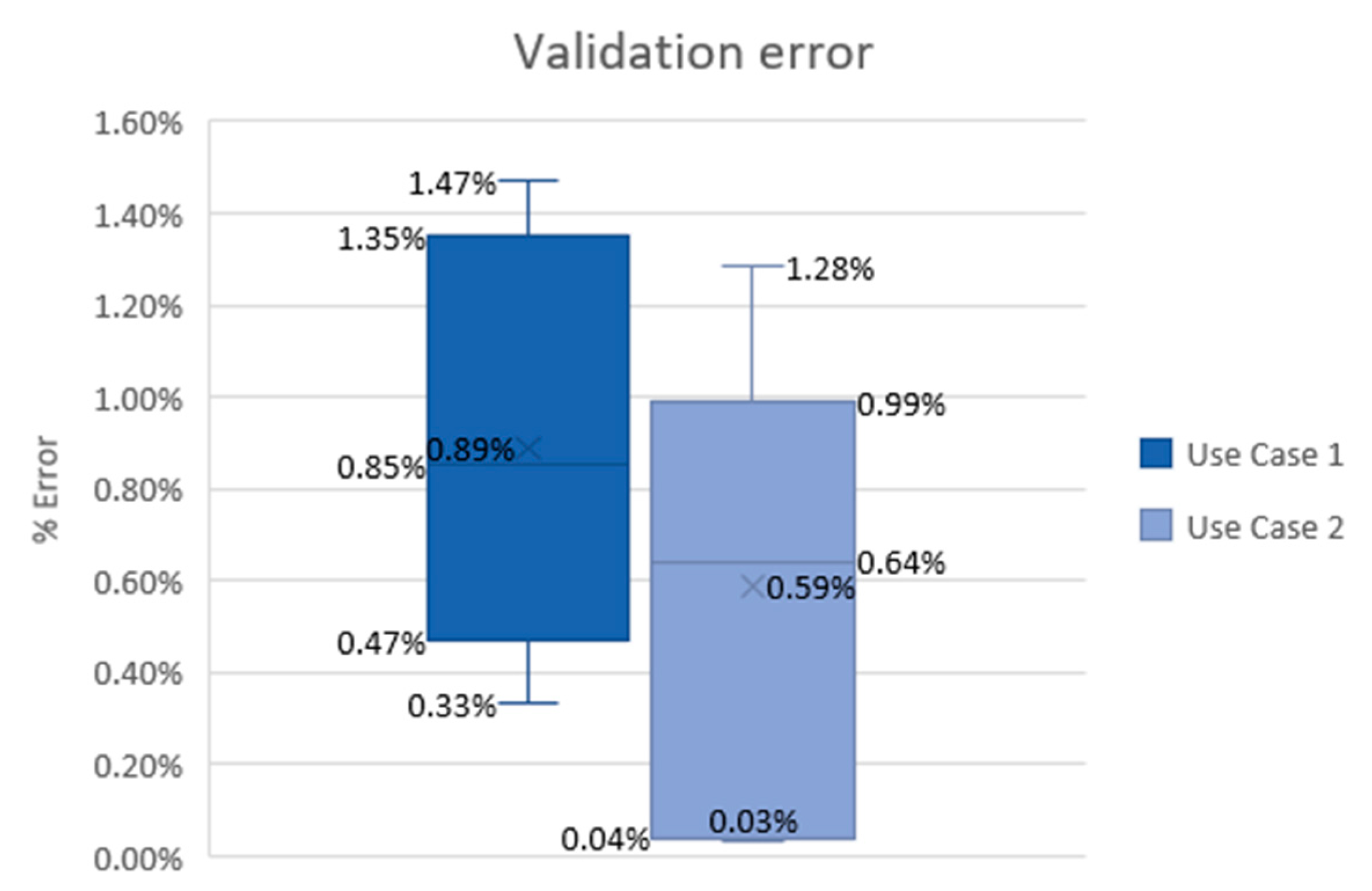
| Scenary 1-High Occupancy | 90% | 93.527% | 93.860% | 0.333% | 97.198% | 95.915% | 1.283% |
| 80% | 95.165% | 93.856% | 1.309% | 96.706% | 95.815% | 0.891% | |
| 70% | 92.374% | 93.845% | 1.471% | 96.642% | 95.824% | 0.818% | |
| Scenary 2-Low Occupancy | 40% | 94.584% | 93.959% | 0.625% | 96.381% | 95.917% | 0.464% |
| 30% | 93.434% | 93.948% | 0.514% | 95.946% | 95.913% | 0.033% | |
| 20% | 95.235% | 94.153% | 1.082% | 95.879% | 95.918% | 0.039% | |
Publisher’s Note: MDPI stays neutral with regard to jurisdictional claims in published maps and institutional affiliations. |
© 2022 by the authors. Licensee MDPI, Basel, Switzerland. This article is an open access article distributed under the terms and conditions of the Creative Commons Attribution (CC BY) license (https://creativecommons.org/licenses/by/4.0/).
Share and Cite
Delgado-Aguilera Jurado, R.; Gómez Comendador, V.F.; Zamarreño Suárez, M.; Pérez Moreno, F.; Verdonk Gallego, C.E.; Arnaldo Valdés, R.M. Assessment of Potential Conflict Detection by the ATCo. Aerospace 2022, 9, 522. https://doi.org/10.3390/aerospace9090522
Delgado-Aguilera Jurado R, Gómez Comendador VF, Zamarreño Suárez M, Pérez Moreno F, Verdonk Gallego CE, Arnaldo Valdés RM. Assessment of Potential Conflict Detection by the ATCo. Aerospace. 2022; 9(9):522. https://doi.org/10.3390/aerospace9090522
Chicago/Turabian StyleDelgado-Aguilera Jurado, Raquel, Víctor Fernando Gómez Comendador, María Zamarreño Suárez, Francisco Pérez Moreno, Christian Eduardo Verdonk Gallego, and Rosa María Arnaldo Valdés. 2022. "Assessment of Potential Conflict Detection by the ATCo" Aerospace 9, no. 9: 522. https://doi.org/10.3390/aerospace9090522
APA StyleDelgado-Aguilera Jurado, R., Gómez Comendador, V. F., Zamarreño Suárez, M., Pérez Moreno, F., Verdonk Gallego, C. E., & Arnaldo Valdés, R. M. (2022). Assessment of Potential Conflict Detection by the ATCo. Aerospace, 9(9), 522. https://doi.org/10.3390/aerospace9090522