
Two-Level Hierarchical-Interaction-Based Group Formation Control for MAV/UAVs

Equipment Management and UAV Engineering College, Air Force Engineering University, Xi’an 710051, China
*
Author to whom correspondence should be addressed.
Aerospace 2022, 9(9), 510; https://doi.org/10.3390/aerospace9090510
Submission received: 9 August 2022
/
Revised: 7 September 2022
/
Accepted: 9 September 2022
/
Published: 14 September 2022
(This article belongs to the Special Issue Learning-Based Intelligent Control in Aerospace Applications)
Abstract
:Cooperative group formation control of manned/unmanned aircraft vehicles (MAV/UAVs) using a hierarchical framework can be more efficient and flexible than centralized control strategies. In this paper, a two-level hierarchical-interaction-based cooperative control strategy is proposed for the MAV/UAVs group formation. At the upper level, combined with the nonlinear disturbance observer (NDO) and dynamic surface control (DSC) algorithm, a trajectory tracking problem with external disturbances for MAV is formulated. At the lower level, the leader-following formation controller is utilized to deal with the sub-formation keeping control problem for UAVs, based on the sliding mode disturbance observer and fast terminal sliding mode control law, and the robust performance and control accuracy are effectively improved. Moreover, the overall stability of the MAV/UAVs system is demonstrated using Lyapunov theory. The proposed approach is evaluated by simulation under the ground penetration combat mission for MAV/UAVs, and the performance is compared with that of other control strategies.
1. Introduction
The manned/unmanned aircraft vehicles (MAV/UAVs) formation cooperation can give full play to the advantages of MAV/UAVs system, such as higher combat efficiency and flexible tactics. This new combat style will have a disruptive impact on future air warfare, with great operational potential and military application prospects [1,2]. Facing the complex battlefield environment, a large number of low-cost, single-function unmanned wingmen cooperating with MAV has become a research topic of widespread concern at home and abroad [3].
To meet the battlefield situation and mission demands when MAV/UAVs formation cooperate to perform combat missions, it is necessary to form and maintain a specific formation to maximize the overall advantages and improve the mission capability rate. As the key to MAV/UAVs formation flight, the control strategies of formation keeping mainly include four types: leader-following approach [4,5,6], virtual structure approach [7,8], behavior approach [9,10] and consensus theory [11,12,13]. Compared with conventional multi-UAVs formation, the MAV is both the leader and main decisionmaker of the whole formation during MAV/UAVs flight [14]. The pilot manipulates the MAV to follow the desired trajectory, and the unmanned wingmen follow the trajectory of the leader at a certain relative distance so as to achieve the desired formation. In [15,16,17], the author investigated the problem of formation keeping based on the leader-following approach. Inspired by the leader–follower control framework, a formation keeping control law for wingman is designed in [18], which achieves the cooperative formation flight between MAV and multi-UAVs. In [19], formation flight demonstration experiments were conducted for F-15 manned aircraft and T-33 jet, and the reliable wingman was able to maintain the desired formation with the manned aircraft when the manned aircraft performed maneuvers. It is worth noting that the formation scale in [16,17,18,19] is small and all the members keep a single formation, which has certain limitations for joint air warfare with multi-mission demands. Therefore, a good control scheme is required to improve combat efficiency and tactical flexibility.
Facing the complex battlefield environment, if multi-UAVs can be decomposed into several task groups, the cooperative implementation of electronic countermeasures, target search, fire cover and weapon launch will significantly improve the survivability and combat efficiency of formation under the interaction of the MAV, inter-subgroup and intra-subgroup [20]. Professor Dong and his team first proposed the concept of group formation control [21] and analyzed the sufficient conditions and constraints of group formation for second-order multi-agent systems. In [22], they studied the group formation control problem of second-order multi-agent systems with switching directed topology. To control the macroscopic motion of the formation as a whole, the group formation control protocol for followers based on the leader-following approach is designed in [23], and the leader provides the formation reference trajectory to realize the time-varying formation tracking control of multiple formations. However, the stability of the control system under the influence of disturbances was not analyzed in [21,22,23], considering that the formation system will inevitably be affected by external disturbance, which will increase the challenge of our study about group formation tracking control problem.
Early disturbance control methods, such as PID and linear quadratics, cannot meet the demand for high precision control; in order to improve the control accuracy of the formation control system with external disturbances, the main control methods commonly mentioned in literature are robust control [24], sliding mode control [25,26] and adaptive backstepping control [27]. As noted in [27], the adaptive backstepping approach is applied to handle the inevitable parametric uncertainties and improve the stability of fixed-wing unmanned aerial vehicle swarm formations. Due to the complex design, uncertain disturbances, and slower response speed of the controller, in contrast, the nonlinear disturbance observer (NDO) can estimate the disturbance and compensate it through feedforward, so it reflects faster and has strong practical application prospects. In [28], it improves the robustness and control accuracy by estimating and compensating the disturbance terms based on the NDO. Sliding mode control with the NDO method is combined in [29,30] to solve the UAV formation tracking control problem with external disturbances. In [31], a backstepping (BS) control strategy based on a sliding mode disturbance observer is proposed, and the double power reaching law is used to design the sliding mode controller, which improves the error convergence speed and enhances the system anti-disturbance performance. Motivated by the facts stated above, this paper introduces the sliding mode control with the NDO approach to deal with cooperative group formation control with external disturbances.
In summary, group formation tracking control has significant advantages for solving the cooperative control problem with multi-mission formation. However, there are few studies on this control problem, and it is mainly applied in second-order multi-agent systems. Regarding the MAV/UAVs group formation tracking control, there is still a gap in this area due to its frontier state and complexity. Motivated by the aforementioned results, in this paper, we propose a group formation control strategy for MAV/UAVs formation control system, responding to the future multi-mission cooperative formation tracking control problem with strong disturbance environment. Therefore, the main contributions of this paper are as follows:
(1) In contrast to [18,19], which only focuses on a single MAV/UAVs formation, we propose a two-level hierarchical-interaction-based control strategy for the MAV/UAVs group formation wherein we divide the UAVs into group leaders and followers incorporating the group formation interaction topology.
(2) In order to ensure that MAV tracks pre-defined trajectories while effectively suppressing external disturbances, a dynamic surface control (DSC) method based on a NDO is proposed. Meanwhile, the fast terminal sliding mode control (FTSMC) is introduced to design formation controllers for each UAV, which improves the convergence of formation errors and the accuracy of disturbance estimation.
(3) Compared with the fixed configuration-based formations in [22,23], the proposed method can adjust the desired formation configuration according to the mission requirements.
The remaining parts of this paper are organized as follows. Section 2 formulates the preliminaries and problem formulation. The details of the controller design methods and stability analysis are presented in Section 3. Then, the numerical simulation analysis is presented in Section 4. Finally, the conclusion is summarized in Section 5.
Notations: Throughout this paper, denotes the Euclidean n-space, denotes the zero matrix with size , and and stand for the maximum and minimum eigenvalues of the matrix, respectively. denotes the Euclidean norm of the vector, and denotes the signum function.
2. Preliminaries and Problem Formulation
2.1. Mathematical Model of MAV
Consider the external disturbances, the model of MAV can be expressed as follows [32]:
where denote the positions of the MAV in the inertia frame, and are the mass and gravity constant, respectively. , , and are the bank angle, heading angle, and flight-path angle, respectively. represents the airspeed of the MAV. , , and are the thrust, lift and drag, respectively. , and are the velocities of external disturbances along the , , and axes, respectively. The mathematical model of MAV is shown in Figure 1.
By defining , , , and taking , , the model of MAV can be formulated as
where , and are given by
2.2. Mathematical Model of UAVs
The UAV swarm is assumed to be comprised of n fixed-wing UAVs, and we suppose that there are m group leaders and n-m followers. To facilitate the group formation controller design with external disturbances, the second-order integrator model of UAVs is given by [33]:
where denotes the position of the i-th UAV in the inertia frame, is a control signal commanded by a controller, and , and are the airspeed and external disturbances, respectively.
Assumption 1.
and vary slowly, so it is reasonable to suppose that,, the disturbances are all bounded and satisfying,, where, are positive constants.
The following lemmas are useful for the stability of the system in the paper.
Lemma 1 [34].
(Yong’s inequality) For any vector,, supposeandsuch that,is any positive constant, then we have. In particular, if,is an arbitrary positive constant, then.
2.3. Group Formation Interaction Topology
Let the directed graph represent interaction topology among the agents in the formation system [37], where and stand for the node set and edge set, respectively. A directed edge represents that the agent j can receive information from the agent i. The connection weight between the nodes and is denoted by , and the weight matrix is defined as if and otherwise. Note that for all agents. The Laplacian matrix is defined as , where and . A directed graph has a spanning tree and is globally reachable if there exists at least one node called the root node that has a directed path to all the other nodes [38].
Consider that the UAV swarm system consists of m group leaders and n-m followers. Let and represent the leader and follower subscript sets, respectively. Then the corresponding Laplacian matrix can be defined as [39,40]:
where characterizes the interactions from the MAV to group leaders of UAVs. Here, we define , if the group leaders can receive the information from the MAV, then , otherwise . describes the mutual interaction between the subgroups, represents the intra-subgroup interaction between leader and its followers, and denotes the interaction among the followers.
Assumption 2.
The formation consists of the leader (MAV) and n followers (UAVs), a spanning tree exists in the graph, and the MAV is a globally reachable node, then, the MAV is connected to all the other nodes in the graph.
Assumption 3.
For any subgroup of UAV, it contains a group leader andfollowers, where,. In this case, the group leader only receives information from the MAV and other subgroup leaders; followers can perform its mission by receiving information from its group leader and other followers in the same subgroup. It is worth noting that followers in different subgroups have no connections with each other, and they can only receive information from its subgroup leader and other followers in the same subgroup.
Remark 1.
In order to control the macroscopic movement of sub-formation, the information of MAV is used to characterize the formation reference information. The nodein the Laplacian matrix is added to describe the ability of group leader to access the desired position and velocity information of MAV.
2.4. Group-Based Hierarchical Structure of MAV/UAVs
The hierarchical framework can be more efficient and flexible to deal with complicated systems than centralized control strategies. The design idea is inspired by [17], and the group-based hierarchical structure is designed for the MAV/UAVs group formation. In this structure, all the UAVs are divided into several independent groups, which in the same subgroup can cooperate to complete the same subtask of complicated missions. For any subgroup of UAV, it contains a group leader and followers. Figure 2 describes the two-level hierarchical-interaction-based cooperative control structure. At the upper level of the structure, the MAV, as the leader of the subgroups, realizes the macroscopic movement, and at the lower level, each subgroup of UAVs is required to form a desired sub-formation through inter-subgroup and intra-subgroup interactions.
As shown in Figure 2, in order to control the macro-trajectory of the formation, we first design a trajectory tracking controller for MAV. The pilot manipulates the aircraft to precisely track the desired trajectory and sends formation parameters to the leader of each subgroup. Then we design a distributed formation keeping controller for group leaders to follow their respective trajectories. Each subgroup of UAVs can obtain the desired position and velocity information from their group leader and neighbors via the communication link. Based on the distributed formation keeping controller, other followers in each subgroup can maintain the desired formation parameters with their neighbors. Thus, the cooperative flight of the whole swarm is realized.
2.5. Group Formation Control Objective
Definition 1.
where,, andare the position of MAV, group leaders and followers of UAVs, respectively. and represent the desired relative position for the g-th subgroup.
Consider MAV and a set of UAVs modeled by Equations (2) and (5); the MAV/UAVs formation system will achieve group formation tracking control if the following equations hold.
Remark 2.
According to Assumption 3, for any group that contains a group leader and UAVs, we let,. If the i-th UAV belongs to the-th subgroup, it can be expressed as, and the node set of the subgroupcan be expressed as, where, .
3. MAV/UAV Group Formation Controllers Design
In this section, the formation controller design process includes two parts, the trajectory tracking controller for MAV, and the distributed formation keeping controller for UAVs. Based on the proposed controllers, the position of the MAV/UAVs converges to their designed trajectory and forms a specified formation.
3.1. MAV Trajectory Tracking Controller Design
To achieve the trajectory tracking control of MAV, the trajectory tracking error is expressed as
where and are the desired trajectory and actual position, respectively.
Taking the time derivatives of (7) yields
Choose the Lyapunov function candidate as
According to (8), taking the time derivatives of (9), one has
Design the virtual control law as
where the gain matrix is the diagonal matrix and all elements are positive constants.
The speed tracking error of MAV is defined as
From (11) and (12), then, (12) can be organized as follows
From (2) and (12), one can obtain
In this section, the dynamic surface control method is used to obtain virtual control signal , and the first-order filter is given by
where and are the positive design parameter and the output of the filter, respectively. could be regarded as by choosing appropriate .
Define the following filtering error as
Considering the speed tracking error and filtering error of MAV, choose the Lyapunov function candidate as
Take the time derivative of and after substituting (14) into (17), we can obtain
To estimate the disturbance of (2) and weaken its effect on trajectory tracking, the nonlinear disturbance observer is designed as [28]:
where, , and are the states, and , , is the estimated value of the disturbance, is a positive odd constant.
According to (18), the trajectory tracking controller is designed as
where the gain matrix is the diagonal matrix and all elements are positive constants.
Theorem 1.
For the system (2), consider a closed-loop system consisting of the virtual control law (11), the first-order filter (15), the disturbance observer (19), and the actual control law (20) for trajectory tracking control of the MAV. If Assumption 1 holds, then for any positive constant, given the initial conditions, there exist adjustable parameters , , and , the signals of the closed-loop system are consistently bounded while achieving the position tracking error , and velocity tracking error converges in a neighborhood near the origin.
3.2. UAVs Formation Controller Design
In this section, the sub-formation keeping control of UAVs under external disturbances is tackled. To address this complicated issue, we first construct the trajectory tracking error for group leaders and followers. Then, the distributed formation keeping controller is designed based on the sliding mode disturbance observer and fast terminal sliding mode control law, which achieve the expected sub-formation and trajectory tracking for UAVs. The estimates of disturbances are compensated through feedforward, which enhances the preferable tracking performance for each UAV.
Before moving forward, define the position tracking error for each group leader UAV as
Choose the Lyapunov function candidate as
According to (21), taking the time derivative of (22) yields
Then, design the virtual control law of group leaders as
Define the velocity tracking error as
Therefore, substituting (24) and (25) into (23) yields
Similarly, the position tracking error of followers in any g-th group can be written by
Choose the Lyapunov function candidate as
Taking the time derivative of (28) gives
Then, the virtual control law is designed as
where , then define the speed tracking error as
Thus, the time derivative of can be expressed as
To estimate and compensate for the external disturbance, the nonlinear disturbance observer is employed based on the improved sliding mode differentiator for the group leaders and their followers, which is given by [30]
where and are the estimates of and , respectively, is the auxiliary variable, and are the design parameters, and and are the terminal attractor parameters, and satisfy . To facilitate the controller design and obtain the virtual control law of UAVs, the first-order filter is given by
where is a positive design parameter, and is the output of the filter. Then, define the filter error as
Considering the speed tracking error and disturbance estimation error, define a new set of errors as
where , is the forward speed tracking error, and is the estimation of external disturbance.
Remark 3 [41].
Ifchanges slowly, the error,can converge to zero in finite time, and smooth estimation of the disturbance can be achieved.
In order to make the speed tracking error converge to zero quickly in a limited time, the fast terminal slide surface is designed as [42]
where is the position tracking error, , , , . and are positive odd constants and satisfies .
The time derivative of (37) yields
Then, the global fast sliding mode control law is designed as
where and are diagonal matrices, and all elements are positive constant. and are positive odd constants and satisfy .
Theorem 2.
For the system (5), consider a closed-loop system consisting of the virtual control law (24) and (30), the first-order filter (34), the disturbance observer (33), and the actual control law (39). If assumption 1 exists, for an arbitrary constant , given the initial conditions , the appropriate parameters can be chosen so that the estimates of the disturbance converge to the actual disturbance, while the position tracking errors (21) and (27) and the velocity tracking errors (25) and (31) will converge in a neighborhood near the origin.
3.3. Stability Analysis
3.3.1. Stability Analysis of Theorem 1
Proof of Theorem 1.
Define the observation error of the NDO as:
According to (19), the time derivative of (40) can be obtained:
Choose the Lyapunov function candidate as
Taking the time derivative of (42) gives
It follows that the disturbance observation error is bounded and can converge to zero.
According to (41), we obtain
As can be seen from (44), the convergence rate and observation performance of NDO depend on the appropriate parameters and , which can lead to converge to the actual disturbance . It demonstrates that the larger observer parameters can improve the convergence rate. However, when the parameters selected are too large, the nonlinear disturbance observer cannot estimate the estimation of external disturbance accurately, and it leads to undesirable chattering [28,31].
According to (15) and (16), we can obtain
Therefore, Equation (17) can be organized as
where is the non-negative continuous function and satisfies .
Choose the Lyapunov function candidate as
It can be derived from Lemma 1 that
According to (18), the trajectory tracking controller (20) of MAV, the time derivative of (47) can be obtained
where ,, and , then we can guarantee that . It can be derived from Lemma 1 that , then .
According to Lemma 2, Equation (50) can be obtained:
From inequality (51), it is known that . Therefore, it can be concluded that and are bounded. The tracking error can converge to arbitrarily small neighborhoods containing zero by setting to be sufficiently large, then , as . □
3.3.2. Stability Analysis of Theorem 2
Proof of Theorem 2.
Choose the Lyapunov function candidate as
By recalling Equation (38), the time derivative of is given by
From the UAV formation control law (39), we can obtain
where , , and are positive constant. It can be derived from Lemma 1 that will converge to zero in finite time, so is bounded. Since is even, , and the tracking error and will converge in finite time.
Choose the Lyapunov function candidate as
Taking the time derivative of , one has
According to (34) and (35), we can obtain , thus
where is a non-negative continuous function.
It can be derived from Lemma 1 that
By recalling Equation (56) and inequality (57), one has
where . If we take , , then we can ensure that . It can be known from Theorem 2 that , thus . According to Lemma 2, it can be achieved that
Hence, it is proved that all of the signals in the closed-loop system are bounded, and the position tracking errors (21) and (27), and the velocity tracking errors (25) and (31) can converge to arbitrarily small neighborhoods containing zero as by setting to be sufficiently large. Then , , , , and . Therefore, the proposed controller can achieve the desired formation of MAV/UAVs. □
4. Applications: Penetration and Assault Missions of MAV/UAVs
4.1. Simulation Scenario
In this section, the simulation of MAV/UAVs in coordination missions are given to verify the effectiveness of the group-based hierarchical structure. Let us assume a scenario where MAV commands two subgroups of UAVs to complete electronic interference and air-to-ground attack subtasks, and the operational schematic is shown in Figure 3. Considering the autonomous capability of UAVs, the UAV with higher autonomy in the formation is selected as group leader to receive and transmit instructions so as to reduce the workload of MAV and improve the entire operational efficiency. Then, the UAVs are divided into the interference group and attack group. UAV 1 and UAV 2 are selected as the group leaders, and UAV 3–4 and UAV 5–7 are their followers. The MAV and a swarm of UAVs fly toward the attack zone, and the MAV keeps away from the enemy to command the group leaders. Each UAV in the interference group (UAV1 and UAV 3–4) carries an electronic load to block enemy’s defense system and provide fire cover. In the attack group (UAV2 and UAV 5–7), UAVs are equipped with different types of attack weapons. The UAV 1 transmits the target information to the group leader of group 2 (UAV 2) via the communication link. When the MAV detect the enemy’s stealth target through airborne radar, it sends instructions to UAV 2. Then, they will launch missiles to attack the enemy area, and cooperate with the MAV to attack the enemy area with tactical tactics of pretend and active attack.
In order to verify the effectiveness of the proposed method for group-based formation, all the simulations for MAV and seven UAVs are programmed with MATLAB/Simulink and implemented on a PC with 64GB of RAM and Microsoft Window 10.
The simulation scenario is assumed to be as follows: the MAV (Leader) and seven UAVs () take off and form the desired formation at the height of 7000 m, taking low-altitude flight to covertly penetrate the target area. The MAV flies along the desired trajectory (, , , ) to the target area with initial speed (). It is assumed that there are two group leaders () and seven followers (), the interaction topology related to MAV/UAVs system is given in Figure 4.
The MAV instructs the interference group to fly at a lower altitude immediately and sends information to the group leader (UAV 1, ). At the same time, the pilot orders three electronic UAVs () to use electromagnetic disturbance to suppress the target territory and take tactical actions to avoid the radar search. Assuming that the enemy has turned on the guidance radar to search for incoming targets this moment, UAV 1 commands followers (UAV 3–4) to form a parallel-shape formation under the controller (39) in order to expand the scope of search, and the desired relative positions among UAVs are set as , , . The interference-group shield each other to work together with fake actions, deceive the enemy radar, and lure their radar. When the MAV discovers the target using airborne radar, the group leader UAV (UAV 2, ) of the attack group commands its followers (UAV 5–7, ) to form a trapezoidal-shape formation under the controller (39) in order to perform a coordinated assault mission. The desired relative positions among UAVs are set as , , , . Then the UAVs in different subgroups work together to complete different subtasks of the whole complicated missions with their direct leaders.
In the simulation, the control parameters of MAV are set as , , and the external time-varying disturbance are chosen as . Then, the control parameters of UAVs are selected as follows:, , , , , , , , , , for the nonlinear disturbance observer; and , for the first-order filter. The external time-varying disturbance of UAV is set as , and the initial values of the UAVs are shown in Table 1.
4.2. Results and Analysis
The spatial position of MAV/UAVs (both the group leaders and the followers) are shown in Figure 5, where the state of the MAV (Leader) is denoted by red hexagonal, and the states of subgroup leaders () are marked by solid purple circle and solid black square, the states of followers are indicated by diamonds, inverted triangles and diamonds. It can be observed from Figure 5 that the UAVs of group 1 are located 90 m below other members at s, in order to attract enemy fire and protect them. Figure 6 depicts the overhead view of the MAV/UAVs, which reveals that for s, the UAVs coordinate with their direct leaders and give rise to the parallel-shaped, trapezoidal-shaped formation, respectively.
In order to verify the effectiveness of the trajectory tracking for MAV, two simulations are carried out in the presence of external disturbances. The first simulation is conducted under the DSC and nonlinear disturbance observer based (DSC + NDO) composite controller. The second simulation is carried out under the backstepping (BS + NDO) composite controller, which consists of NDO. The trajectory tracking curves in two simulations are shown in Figure 7, the red line stands for the desired trajectory of the MAV, and the green and blue lines represent the trajectory of proposed controllers, respectively. It can be observed from Figure 7 that, when the trajectory tracking errors reaches the range of near zero, the error under the DSC + NDO controller converges to zero faster than that under the BS + NDO controller. This demonstrates that the introduction of the first-order filter avoids the derivation of virtual control variable and reduces the calculational complexity. As a contrast, under the MAV trajectory tracking controller (20), the satisfactory tracking performance can be achieved in the presence of external disturbances.
Figure 8 shows the position tracking errors of seven UAVs, from which we can find that the position tracking errors are large at the initial moment and all the errors converge to 0 at about 4 s. This means that the desired formation is formed at about 4 s. From Figure 8c, it can be observed that the errors of the z-direction fluctuate suddenly at s. This is due to the fact that the UAVs are decelerating, which results in certain fluctuations in a short period of time, but the tracking error can eventually converge to a neighborhood near the origin as time goes on. Hence, as shown in Figure 8, under the formation keeping controller, the formation configuration can be kept well, even in the presence of external disturbances.
The position tracking error of UAV1 is given in Figure 9. It is observed from Figure 9 that the proposed method (FTSMC + NDO) has better tracking performance than terminal sliding mode composite controller (TSMC + NDO). When the position tracking error is close to the equilibrium state, the error under the FTSMC + NDO controller converges to zero faster than that under the TSMC + NDO controller. Compared with the composite controller (TSMC + NDO) in [42], the tracking performance is evidently improved owing to the introduction of the linear sliding mode in the sliding mode surface. When the position tracking error reaches the small region containing zero, it will converge to zero faster. As shown in Figure 9, the position tracking performance of UAVs remains excellent in the case of the FTSMC controller, and the position tracking errors rapidly adjust to achieve the desired formation configuration.
Figure 10 illustrates the estimation errors of the disturbances from which we can observe that the errors of MAV under composite controller (DSC + NDO) can be converged into a small region containing zero at about s. The estimation errors of UAV1 are displayed in Figure 11. However, when the deceleration is encountered by UAV1 at s, the estimation errors of the z-direction have sharp fluctuations from the small region containing zero. It can be observed from Figure 11 that the disturbance estimation errors can reach the range of near zero at s. Thus, the tracking performance under the presented control scheme maintain the equilibrium point zero, even in the external disturbances encountered by MAV/UAVs.
5. Conclusions
In this paper, a group-based hierarchical control scheme was proposed for MAV/UAVs to solve trajectory tracking and the subgroup formation keeping control problem simultaneously. In contrast to the conventional formation, the proposed control strategy constructed a group formation interaction topology using the relative state information of every UAV to achieve multitarget operations for MAV/UAVs. The NDO-based trajectory tracking controller for MAV was introduced to resist external disturbances and realize the overall macroscopic motion of the subgroup formations. Then, the subgroup formation keeping control problem was formulated for every UAV to improve the convergence rate ang disturbances rejection ability using FTSMC. Moreover, the overall stability of the MAV/UAVs system was analyzed. The effectiveness and superiorities of the proposed control scheme were validated through comparative simulation results.
Author Contributions
Conceptualization, S.L.; methodology, S.L. and H.W.; software, H.W.; validation, S.L.; formal analysis, H.W.; investigation, B.Z.; resources, M.L. and S.L.; data curation, S.L.; writing—original draft preparation, H.W.; writing—review and editing, B.Z. and M.L.; visualization, M.L.; supervision, S.L. and B.Z.; project administration, S.L.; funding acquisition, S.L. and H.W. All authors have read and agreed to the published version of the manuscript.
Funding
This research was funded by Graduate Innovation Practice Fund of Air Force Engineering University (NO. CSJ2021096), the National Natural Science Foundation of China (NO. 61973253) and the key laboratory of National Defense Technology Foundation for Equipment Pre-Research of China (NO. 6142219200301).
Institutional Review Board Statement
Not applicable.
Informed Consent Statement
Not applicable.
Data Availability Statement
Data available on request due to restrictions e.g., privacy or ethical. The data presented in this study are available by contacting the corresponding author. The data are not publicly available due to commercial use.
Conflicts of Interest
The authors declare no conflict of interest.
References
- Fan, J.R.; Li, D.G.; Li, R.P.; Wang, Y. Analysis on MAV/UAV cooperative combat based on complex network. Def. Technol. 2020, 16, 150–157. [Google Scholar] [CrossRef]
- Zhong, Y.; Yao, P.Y.; Zhang, J.Y.; Wan, L. Formation and adjustment of manned/unmanned combat aerial vehicle cooperative engagement system. J. Syst. Eng. Electron. 2018, 29, 756–767. [Google Scholar]
- Yin, S.; He, R.J.; Li, J.J.; Chen, L.; Zhang, S. Research on the operational mode of manned/unmanned collaboratively detecting drone swarm. In Proceedings of the IEEE International Conference on Unmanned Systems (ICUS), Beijing, China, 15–17 October 2021. [Google Scholar]
- Gong, Z.; Zhou, Z.; Wang, Z.; Lv, Q.; Xu, J.; Jiang, Y. Coordinated formation guidance law for fixed-wing UAVs based on missile parallel approach method. Aerospace 2022, 9, 272. [Google Scholar] [CrossRef]
- Rosa, M.R. Leader-Follower synchronization of uncertain Euler-Lagrange dynamics with input constraints. Aerospace 2020, 7, 127. [Google Scholar] [CrossRef]
- Liu, S.G.; Huang, F.P.; Yan, B.B.; Zhang, T.; Liu, R.; Liu, W. Optimal design of multimissile formation based on an adaptive SA-PSO algorithm. Aerospace 2021, 9, 21. [Google Scholar] [CrossRef]
- Zhou, D.J.; Wang, Z.J.; Schwager, M. Agile coordination and assistive collision avoidance for quadrotor swarms using virtual structures. IEEE Trans. Robot. 2018, 34, 916–923. [Google Scholar] [CrossRef]
- He, L.L.; Peng, B.; Liang, X.L.; Zhang, J.Q.; Wang, W.J. Feedback formation control of UAV swarm with multiple implicit leaders. Aerosp. Sci. Technol. 2018, 72, 327–334. [Google Scholar] [CrossRef]
- Alfeo, A.L.; Cimino, M.; Vaglini, G. Enhancing biologically inspired swarm behavior: Metaheuristics to foster the optimization of UAVs coordination in target search. Comput. Oper. Res. 2019, 110, 34–47. [Google Scholar] [CrossRef]
- Qiu, H.X.; Duan, H.B.; Fan, Y.M. Multiple unmanned aerial vehicle autonomous formation based on the behavior mechanism in pigeon flocks. Control Theory Appl. 2015, 32, 1298–1304. [Google Scholar]
- Dong, X.W.; Hu, G.Q. Time-varying formation control for general linear multi-agent systems with switching directed topologies. Automatica. 2016, 73, 47–55. [Google Scholar] [CrossRef]
- Sun, J.; Geng, Z.; Lv, Y.; Li, Z.; Ding, Z. Distributed adaptive consensus disturbance rejection for multi-agent systems on directed graphs. IEEE Trans. Control Netw. Syst. 2018, 5, 629–639. [Google Scholar] [CrossRef]
- Yan, D.H.; Zheng, W.G.; Chen, H. Design a multi-constraint formation controller based on improved MPC and consensus for quadrotors. Aerospace 2022, 9, 94. [Google Scholar] [CrossRef]
- Wu, L.Y.; Han, W. Design of cooperative control system for a carrier-based aircraft/unmanned aerial vehicles formation. In Proceedings of the 5th International Conference on Control Science and Systems Engineering (ICCSSE), Shanghai, China, 14–16 August 2019. [Google Scholar]
- Guezy, H.M. Hybrid consensus-based formation control of fixed-wing MUAVs. Cybern. Syst. 2017, 48, 71–83. [Google Scholar] [CrossRef]
- Zhang, L.; Lu, Y.; Xu, S.D. Multiple UAVs cooperative formation forming control based on back-stepping-like approach. J. Syst. Eng. Electron. 2018, 29, 816–822. [Google Scholar]
- Chen, H.; Wang, X.; Shen, L.; Cong, Y. Formation flight of fixed-wing UAV swarms: A group-based hierarchical approach. Chin. J. Aeronaut. 2021, 34, 504–515. [Google Scholar] [CrossRef]
- Dong, Z.N.; Zhang, M.Y.; Liu, Y. Control method of manned/unmanned aerial vehicle cooperative formation based on mission effectiveness. In Proceedings of the IEEE Chinese Guidance, Navigation and Control Conference (CGNCC), Nanjing, China, 12–14 August 2016. [Google Scholar]
- Waydo, S.; Hauser, J.; Bailey, R.; Klavins, E.; Murray, R. UAV as a reliable wingman: A flight demonstration. IEEE Trans. Control Syst. Technol. 2007, 15, 680–688. [Google Scholar] [CrossRef]
- Ma, Q.; Wang, Z.; Miao, G.Y. Second-order group consensus for multi-agent systems via pinning leader-following approach. J. Frankl. Inst. 2014, 351, 1288–1300. [Google Scholar] [CrossRef]
- Dong, X.W.; Li, Q.D.; Zhao, Q.L.; Ren, Z. Time-varying group formation analysis and design for second-order multi-agent systems with directed topologies. Neurocomputing 2016, 205, 367–374. [Google Scholar] [CrossRef]
- Li, Y.F.; Dong, X.W.; Li, Q.D.; Ren, Z. Time-varying group formation control for second-order multi-agent systems with switching directed topologies. In Proceedings of the 36th Chinese Control Conference (CCC), Dalian, China, 26–28 July 2017. [Google Scholar]
- Li, Y.F.; Dong, X.W.; Li, Q.D.; Ren, Z. Time-varying group formation tracking for second-order multi-agent systems with switching directed topologies. In Proceedings of the Name of the IEEE CSAA Guidance, Navigation and Control Conference (CGNCC), Xiamen, China, 10–12 August 2018. [Google Scholar]
- Yang, D.; Feng, Z.; Sha, R.; Ren, X. Robust control of a class of under-actuated mechanical systems with model uncertainty. Int. J. Control 2019, 92, 1567–1579. [Google Scholar] [CrossRef]
- Xu, J.L.; Hao, Y.P.; Wang, J.J.; Li, L. The control algorithm experimentation of coaxial rotor aircraft trajectory tracking based on backstepping sliding mode. Aerospace 2021, 8, 337. [Google Scholar] [CrossRef]
- Korayem, A.H.; Nekoo, S.R.; Korayem, M.H. Sliding mode control design based on the state-dependent Riccati equation: Theoretical and experimental implementation. Int. J. Control 2019, 92, 2136–2149. [Google Scholar] [CrossRef]
- Muslimov, T.Z.; Munasypov, R.A. Adaptive decentralized flocking control of multi-UAV circular formations based on vector fields and backstepping. ISA Trans. 2020, 107, 143–159. [Google Scholar] [CrossRef] [PubMed]
- Wang, Z.; Wu, Z. Nonlinear attitude control scheme with disturbance observer for flexible spacecrafts. Nonlinear Dyn. 2015, 81, 257–264. [Google Scholar] [CrossRef]
- Fang, X.; Wu, A.; Shang, Y.; Dong, N. A novel sliding mode controller for small-scale unmanned helicopters with mismatched disturbance. Nonlinear Dyn. 2016, 83, 1053–1068. [Google Scholar] [CrossRef]
- Van, M.; Ge, S.S.; Ren, H. Finite time fault tolerant control for robot manipulators using time delay estimation and continuous nonsingular fast terminal sliding mode control. IEEE Trans. Cybern. 2016, 47, 1681–1693. [Google Scholar] [CrossRef]
- Zhang, Z.; Wang, F.; Guo, Y.; Hua, C. Multivariable sliding mode backstepping controller design for quadrotor UAV based on disturbance observer. Sci. China Inf. Sci. 2018, 61, 112207. [Google Scholar] [CrossRef]
- Wu, L.Y.; Han, W.; Zhang, Y. Formation keeping control for a manned/unmanned aerial vehicle formation based on leader-follower strategy. Control Decis. 2021, 36, 2435–2441. [Google Scholar]
- Wang, D.D.; Zong, Q.; Tian, B. Neural network disturbance observer-based distributed finite-time formation tracking control for multiple unmanned helicopters. ISA Trans. 2018, 73, 208–226. [Google Scholar] [CrossRef]
- Yu, Z.Q.; Zhang, Y.M.; Qu, Y.H. Prescribed performance-based distributed fault-tolerant cooperative control for multi-UAVs. Trans. Inst. Meas. Control 2019, 41, 975–989. [Google Scholar] [CrossRef]
- Spooner, J.T.; Maggiore, M.; Ordonez, R. Stable Adaptive Control and Estimation for Nonlinear Systems: Neural and Fuzzy Approximator Techniques, 3rd ed.; John Wiley & Sons: New York, NY, USA, 2004; pp. 31–36. [Google Scholar]
- Chen, L.; Duan, H. Collision-free formation-containment control for a group of UAVs with unknown disturbances. Aerosp. Sci. Technol. 2022, 126, 107618. [Google Scholar] [CrossRef]
- Qin, J.; Yu, C. Cluster consensus control of generic linear multi-agent systems under directed topology with acyclic partition. Automatica 2013, 49, 2898–2905. [Google Scholar] [CrossRef]
- Zhang, Y.; Wang, X.; Wang, S. Three-dimensional formation-containment control of underactuated AUVs with heterogeneous uncertain dynamics and system constraints. Ocean Eng. 2021, 238, 109661. [Google Scholar] [CrossRef]
- Li, D.Y.; Zhang, W.; He, W.; Li, C.; Ge, S.S. Two-layer distributed formation-containment control of multiple Euler–Lagrange systems by output feedback. IEEE Trans. Cybern. 2018, 49, 675–687. [Google Scholar] [CrossRef] [PubMed]
- Hu, J.; Bhowmick, P.; Lanzon, A. Distributed adaptive time-varying group formation tracking for multiagent systems with multiple leaders on directed graphs. IEEE Trans. Control Netw. Syst. 2019, 7, 140–150. [Google Scholar] [CrossRef]
- Levant, A. Higher-order sliding modes, differentiation and output-feedback control. Int. J. Control 2003, 76, 924–941. [Google Scholar] [CrossRef]
- Van, M. An enhanced robust fault tolerant control based on an adaptive fuzzy PID-nonsingular fast terminal sliding mode control for uncertain nonlinear systems. IEEE/ASME Trans. Mechatron. 2018, 23, 1362–1371. [Google Scholar] [CrossRef] [Green Version]
Figure 1.
MAV model.
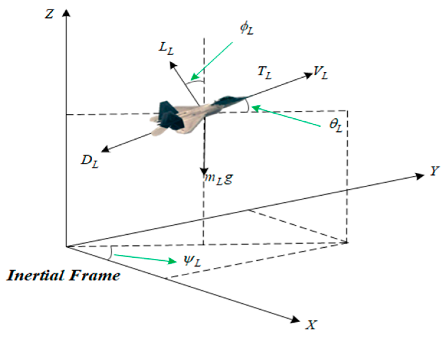
Figure 2.
MAV/UAV group formation control structure.

Figure 3.
Schematic diagram of group-based MAV/UAVs multi-task cooperative operation.
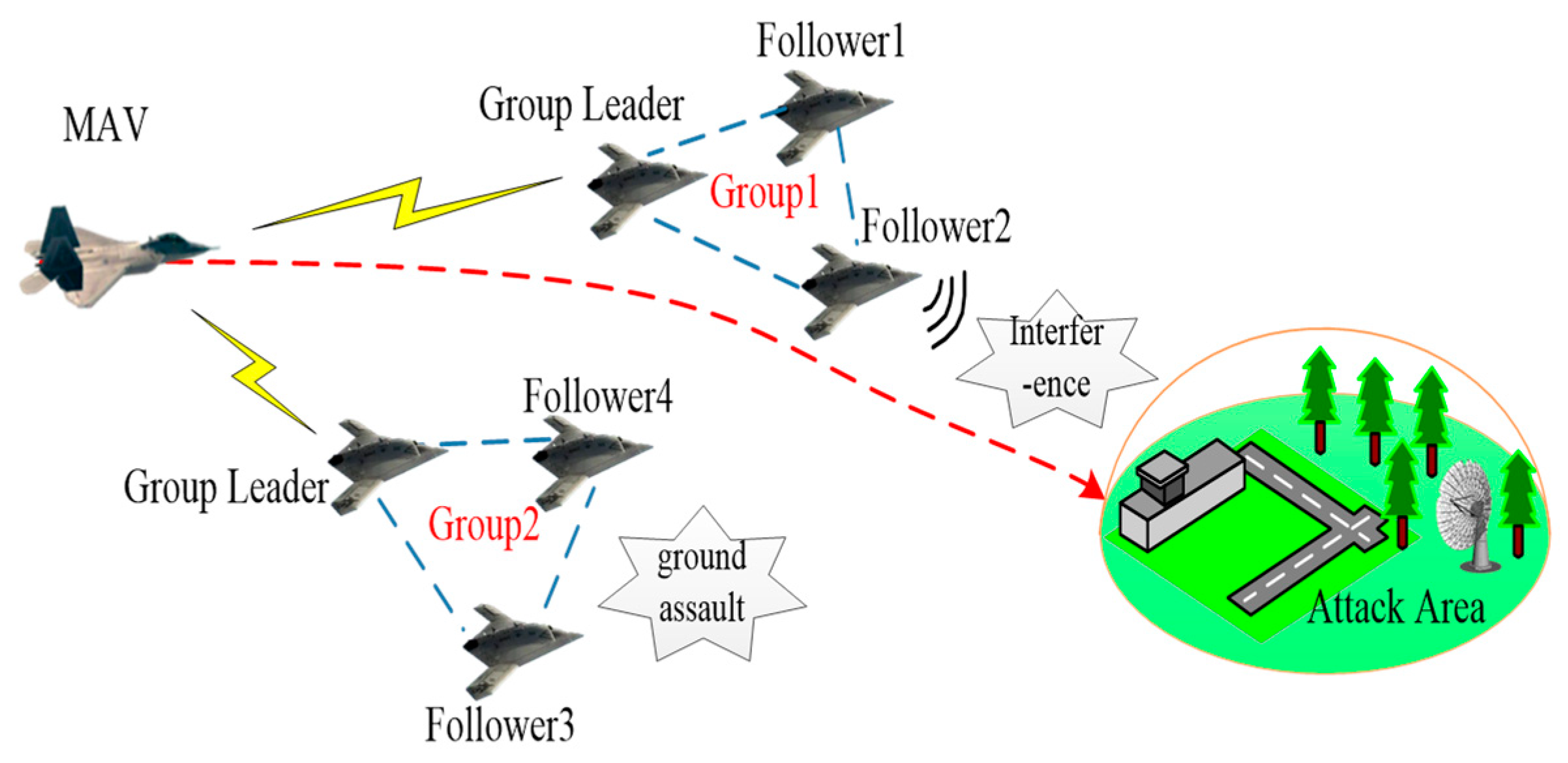
Figure 4.
MAV/UAVs interaction topology.
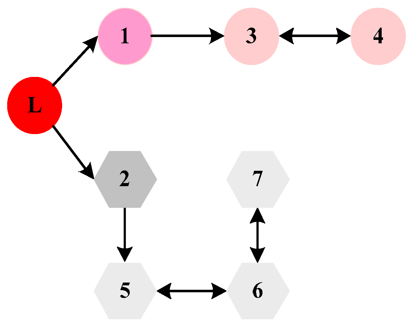
Figure 5.
The 3D-flight diagram of MAV/UAVs group formation.

Figure 6.
Top view of MAV/UAVs group formation.

Figure 7.
MAV trajectory tracking curves: (a) x-direction; (b) y-direction; (c) z-direction.
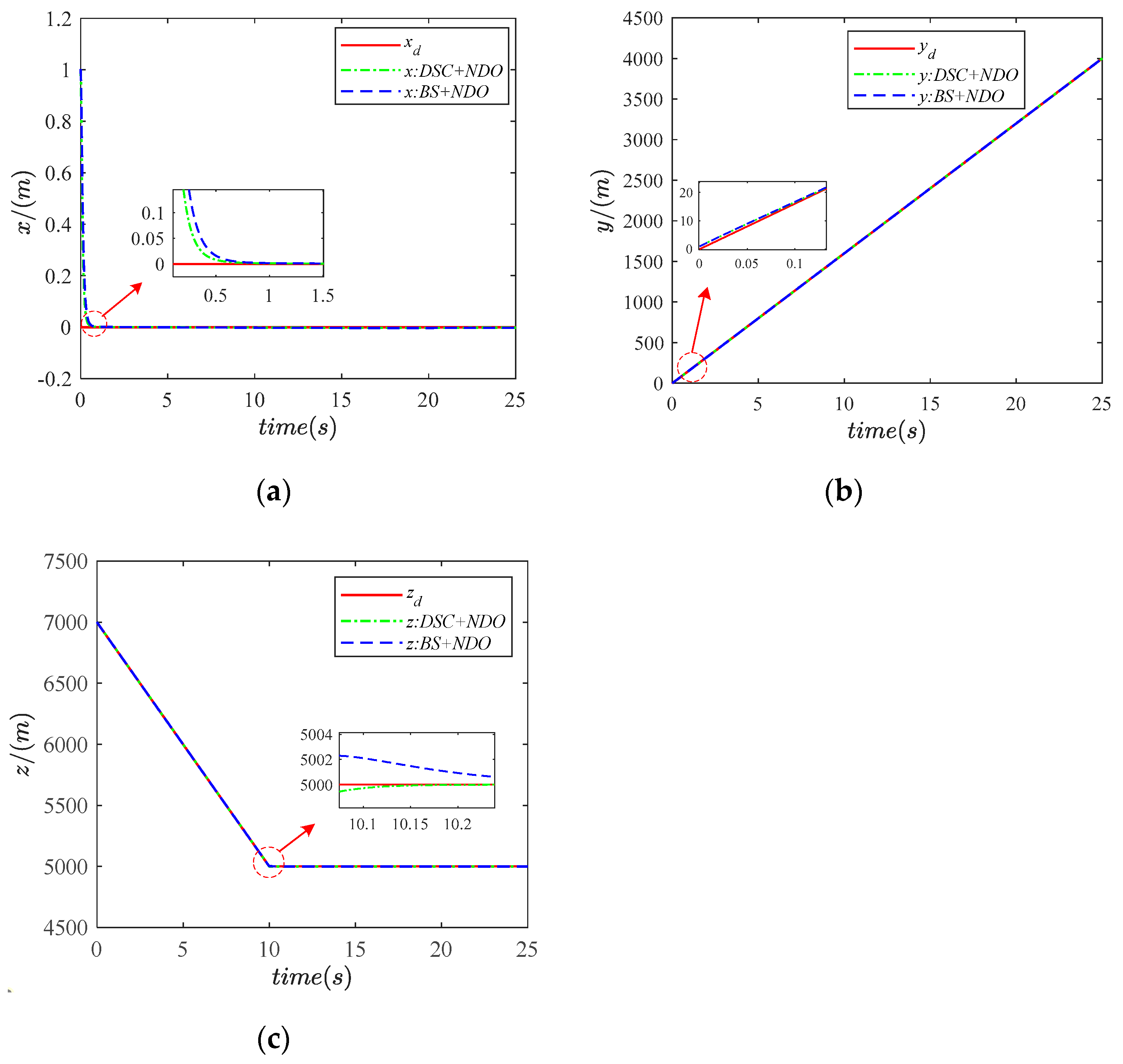
Figure 8.
UAV position tracking error curves: (a) x-direction variation curve; (b) y-direction variation curve; (c) z-direction variation curve.
Figure 8.
UAV position tracking error curves: (a) x-direction variation curve; (b) y-direction variation curve; (c) z-direction variation curve.

Figure 9.
Position tracking error comparison curves of UAV1.
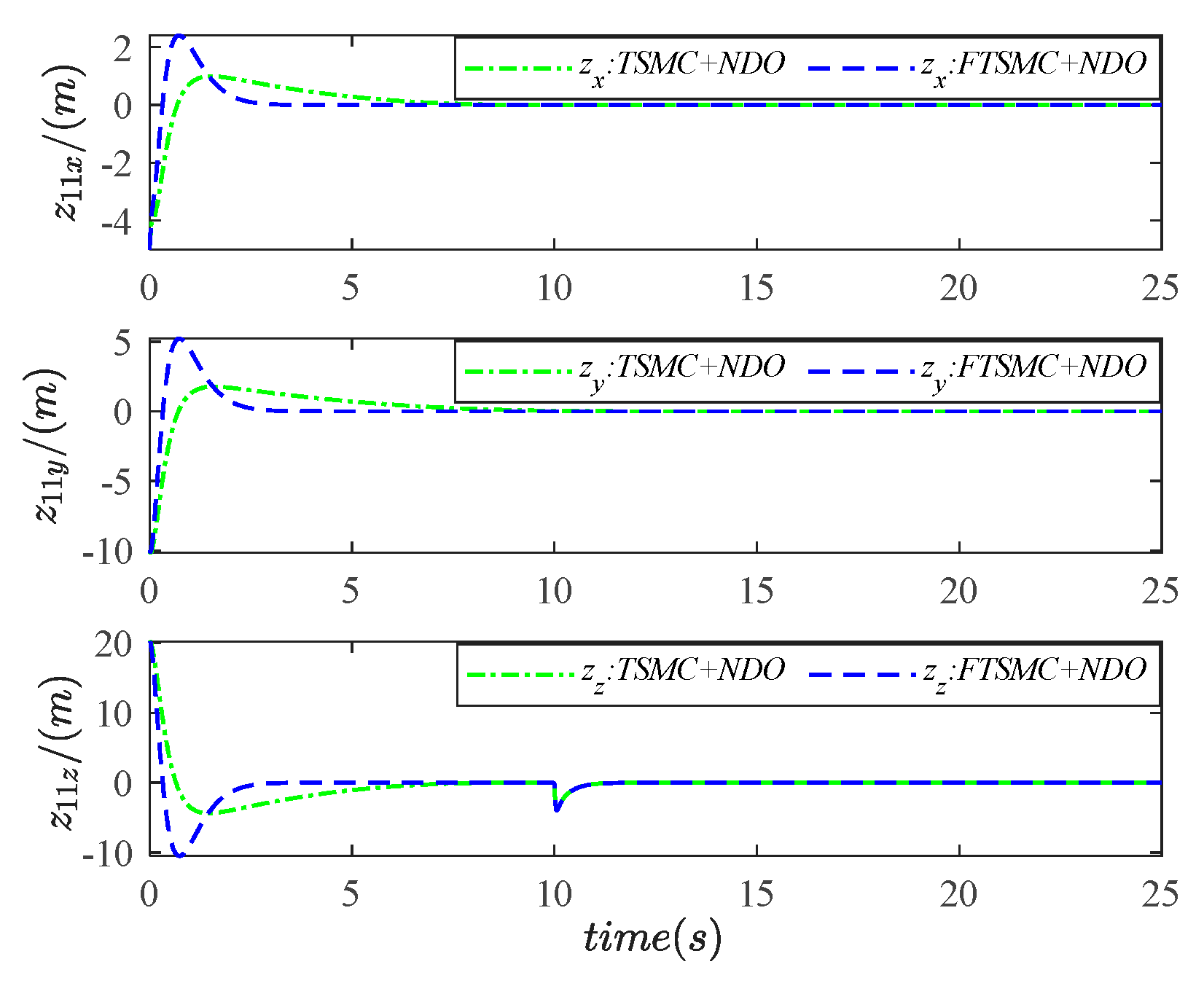
Figure 10.
Disturbance estimation errors of MAV.
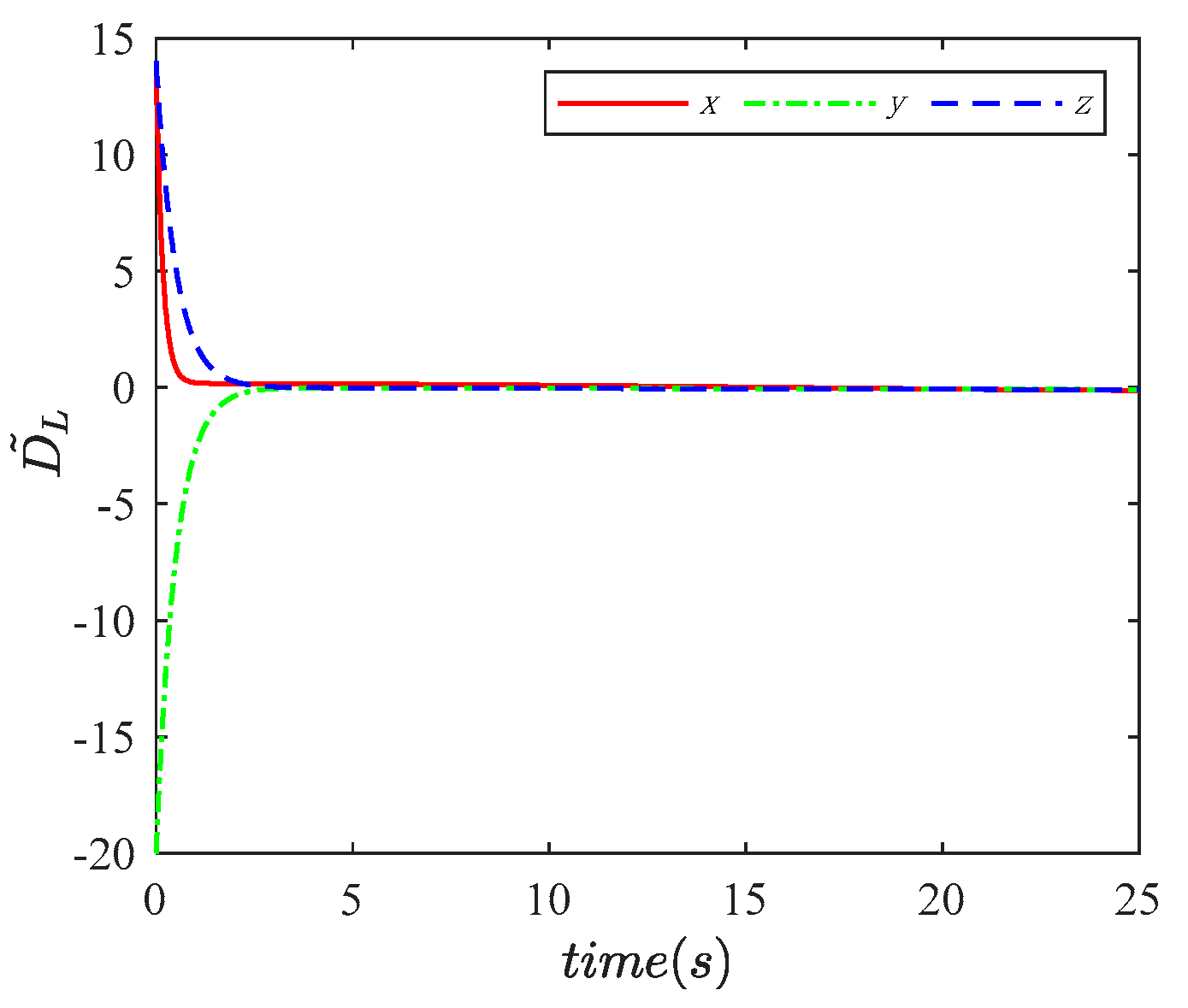
Figure 11.
Disturbance estimation errors of UAV1.


Table 1.
Initial state of the formation.
| Initial Position/(m) | Initial Velocity/(m/s) |
|---|---|
Publisher’s Note: MDPI stays neutral with regard to jurisdictional claims in published maps and institutional affiliations. |
© 2022 by the authors. Licensee MDPI, Basel, Switzerland. This article is an open access article distributed under the terms and conditions of the Creative Commons Attribution (CC BY) license (https://creativecommons.org/licenses/by/4.0/).
Share and Cite
MDPI and ACS Style
Wang, H.; Liu, S.; Lv, M.; Zhang, B. Two-Level Hierarchical-Interaction-Based Group Formation Control for MAV/UAVs. Aerospace 2022, 9, 510. https://doi.org/10.3390/aerospace9090510
AMA Style
Wang H, Liu S, Lv M, Zhang B. Two-Level Hierarchical-Interaction-Based Group Formation Control for MAV/UAVs. Aerospace. 2022; 9(9):510. https://doi.org/10.3390/aerospace9090510
Chicago/Turabian StyleWang, Huan, Shuguang Liu, Maolong Lv, and Boyang Zhang. 2022. "Two-Level Hierarchical-Interaction-Based Group Formation Control for MAV/UAVs" Aerospace 9, no. 9: 510. https://doi.org/10.3390/aerospace9090510
Note that from the first issue of 2016, this journal uses article numbers instead of page numbers. See further details here.