
Shape Sensing for an UAV Composite Half-Wing: Numerical Comparison between Modal Method and Ko’s Displacement Theory


Abstract
:1. Introduction
2. Summary of the Shape-Sensing Methods
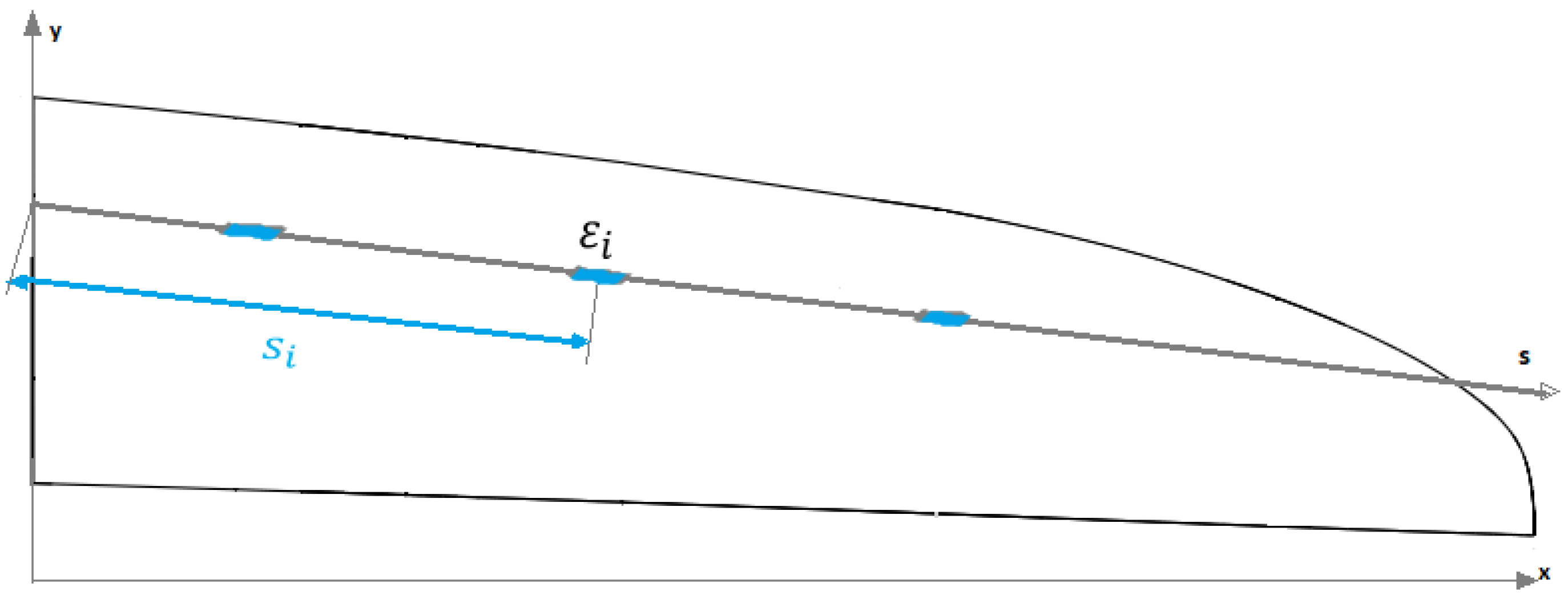
2.1. Ko’s Displacement Theory
2.2. Modal Method
3. Multirotor UAV
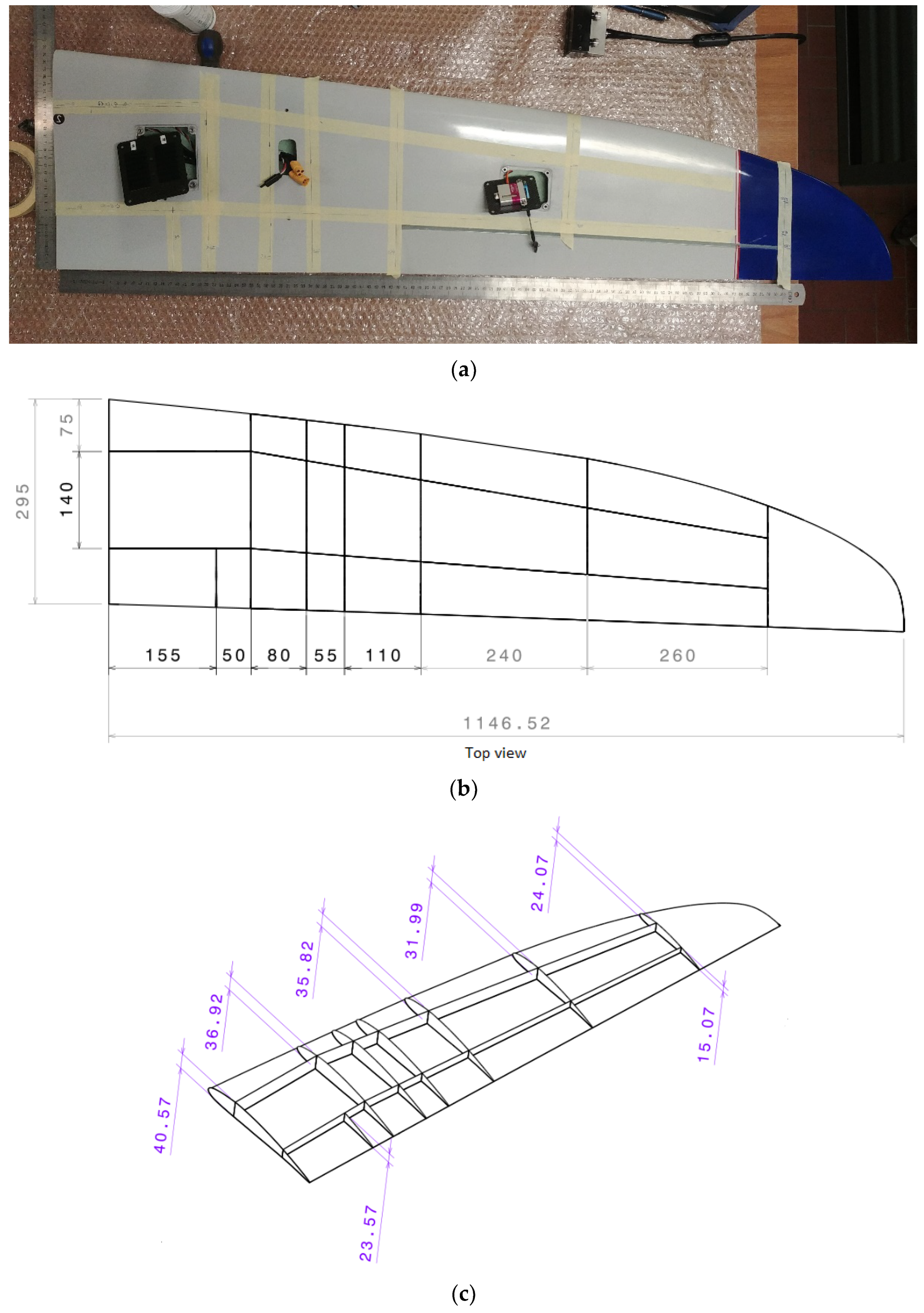
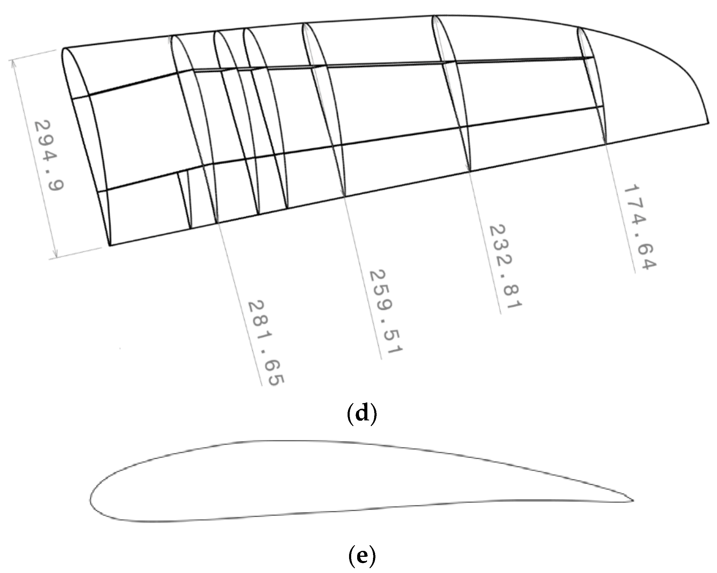
3.1. Geometry and Material Properties
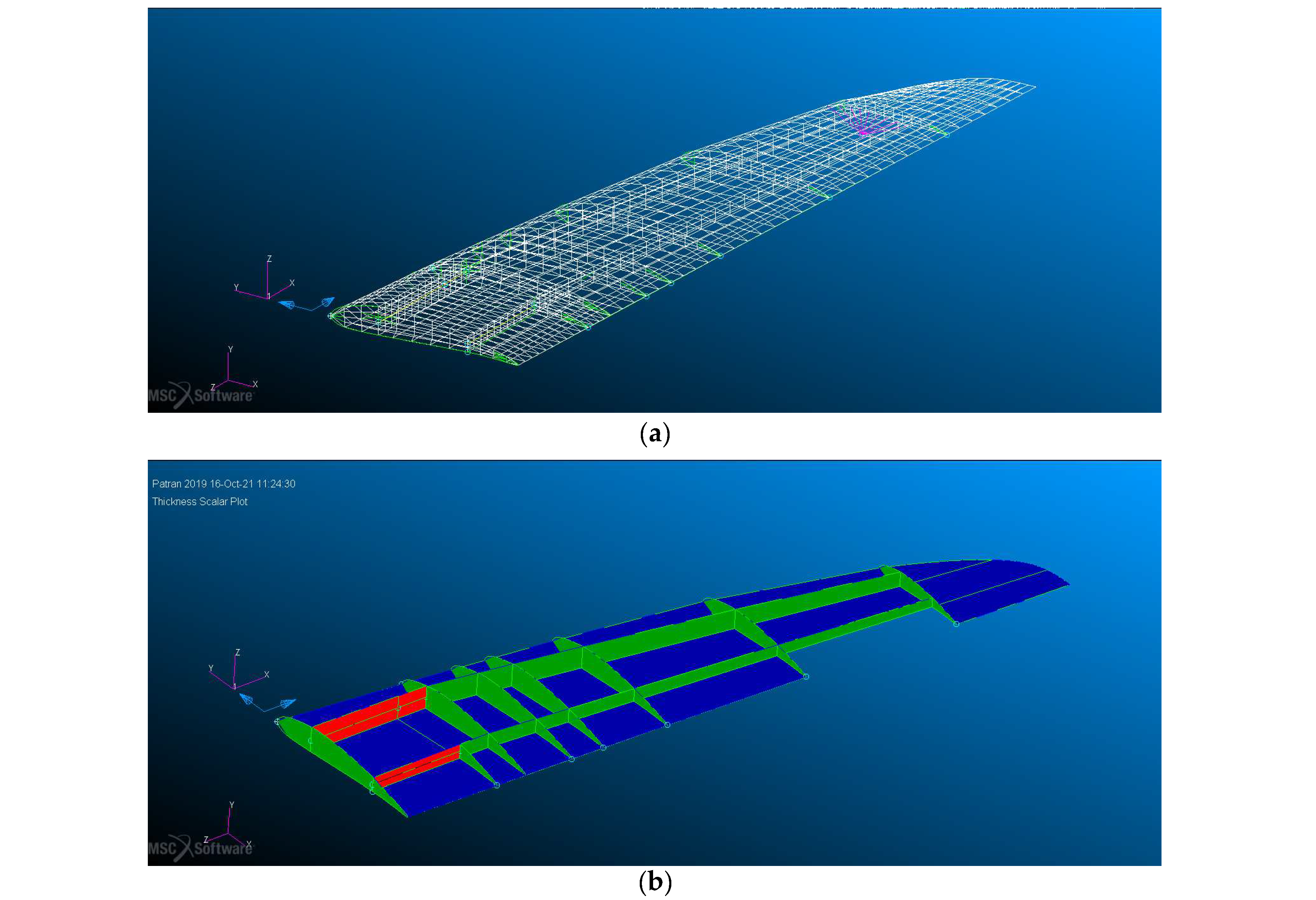
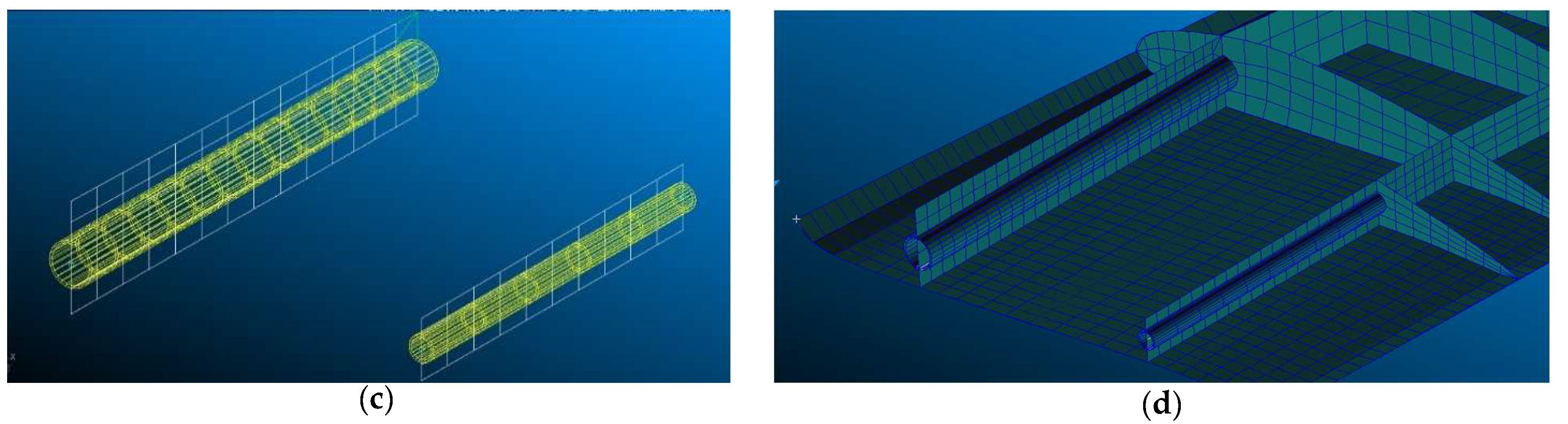
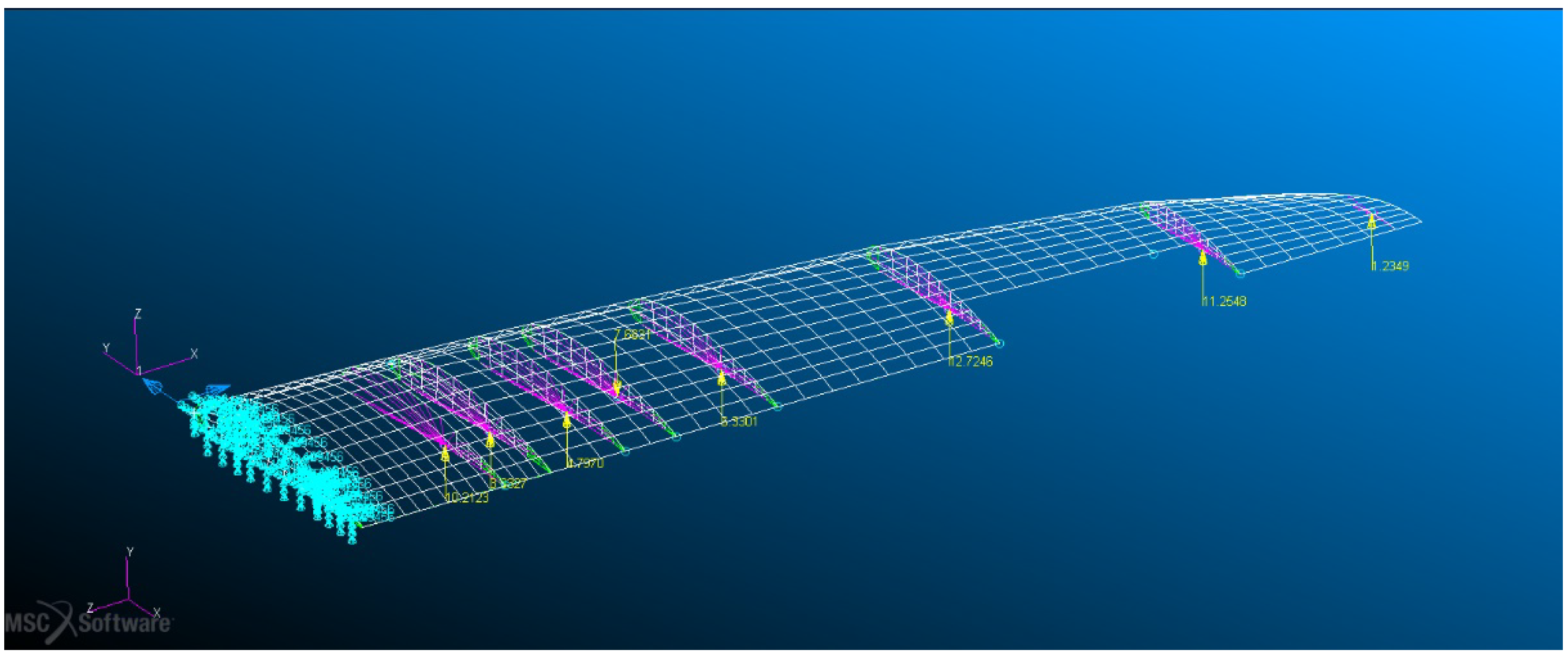
3.2. Half-Wing Finite Element Model
4. Results
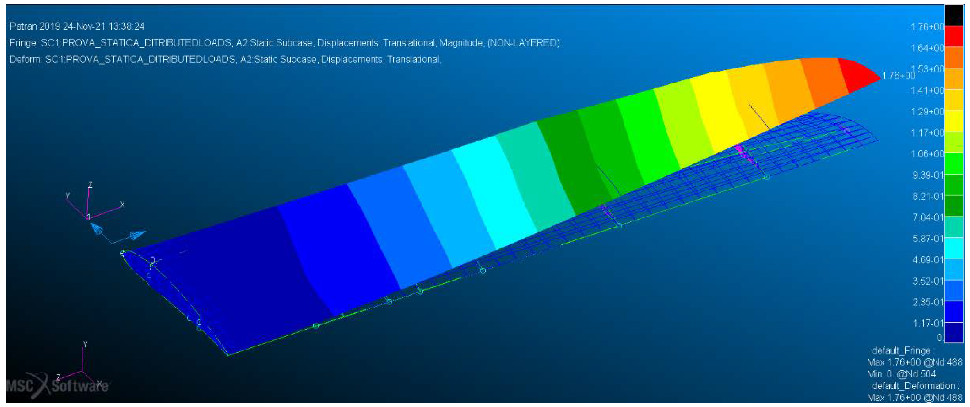
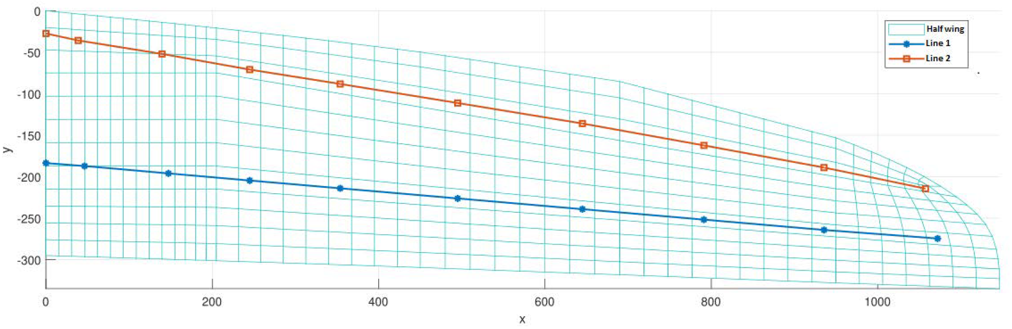
4.1. Shape-Sensing Comparative Investigation
4.2. Enhancement of the Modal Method results
5. Conclusions
Author Contributions
Funding
Informed Consent Statement
Data Availability Statement
Acknowledgments
Conflicts of Interest
References
- Gherlone, M.; Cerracchio, P.; Mattone, M. Shape sensing methods: Review and experimental comparison on a wing-shaped plate. Prog. Aerosp. Sci. 2018, 99, 14–26. [Google Scholar] [CrossRef]
- Evenblij, R.; Kong, F.; Koimtzoglou, C.; Ciminello, M.; Dimino, I. Shape sensing for morphing structures using fiber Bragg grating technology. In Smart Intelligent Aircraft Structures (SARISTU); Springer: Cham, Switzerland, 2016; pp. 471–491. [Google Scholar]
- Brian, J.S.; Dawn, K.G.; Wolfe, M.S.; Mark, E.F. High resolution optical frequency domain reflectometry for characterization of components and assemblies. Opt. Express 2005, 13, 666–674. [Google Scholar]
- Di Sante, R. Fibre Optic Sensors for Structural Health Monitoring of Aircraft Composite Structures: Recent Advances and Applications. Sensors 2015, 15, 18666–18713. [Google Scholar] [CrossRef] [PubMed]
- Ko, W.L.; Tran, V.T.; Richards, W.L. Displacement Theories for In-Flight Deformed Shape Predictions of Aerospace Structures; National Aeronautics and Space Administration, Dryden Flight Research Center: Edwards, CA, USA, 2007. [Google Scholar]
- Akl, W.; Poh, S.; Baz, A. Wireless and distributed sensing of the shape of morphing structures. Sens. Actuators A Phys. 2007, 140, 94–102. [Google Scholar] [CrossRef]
- Bogert, P.; Haugse, E.; Gehrki, R. Structural shape identification from experimental strains using a modal transformation technique. In Proceedings of the 44th AIAA/ASME/ASCE/AHS/ASC Structures, Structural Dynamics, and Materials Conference, Norfolk, VA, USA, 7–10 April 2003. [Google Scholar]
- Foss, G.; Haugse, E. Using modal test results to develop strain to displacement transformations. In Proceedings of the 13th International Modal Analysis Conference, Nashville TN, USA, 13–16 February 1995. [Google Scholar]
- Tessler, A.; Spangler, J.L.; Gherlone, M.; Mattone, M.; Di Sciuva, M. Real-Time Characterization of Aerospace Structures Using Onboard Strain Measurement Technologies and Inverse Finite Element Method; National Aeronautics and Space Administration Hampton Va Langley Research Center: Hampton, VA, USA, 2011. [Google Scholar]
- Tessler, A.; Spangler, J.L. An inverse FEM for application to structural health monitoring. In Proceedings of the 14th US National Congress of Theoretical and Applied Mechanics, Blacksburg, VA, USA, 23–28 June 2002. [Google Scholar]
- Tessler, A.; Spangler, J.L. A least-squares variational method for full-field reconstruction of elastic deformations in shear-deformable plates and shells. Comput. Methods Appl. Mech. Eng. 2005, 194, 327–339. [Google Scholar] [CrossRef]
- Bruno, R.; Toomarian, N.; Salama, M. Shape estimation from incomplete measurements: A neural-net approach. Smart Mater. Struct. 1994, 3, 92–97. [Google Scholar] [CrossRef]
- Mao, Z.; Todd, M. Comparison of shape reconstruction strategies in a complex flexible structure. In Sensors and Smart Structures Technologies for Civil, Mechanical, and Aerospace Systems; SPIE: Bellingham, WA, USA, 2008. [Google Scholar]
- Esposito, M.; Gherlone, M. Composite wing box deformed-shape reconstruction based on measured strains: Optimization and comparison of existing approaches. Aerosp. Sci. Technol. 2020, 99, 105758. [Google Scholar] [CrossRef]
- Esposito, M.; Gherlone, M. Material and strain sensing uncertainties quantification for the shape sensing of a composite wing box. Mech. Syst. Signal Process. 2021, 160, 107875. [Google Scholar] [CrossRef]
- Ko, W.L.; Richards, W.L.; Fleischer, V.T. Applications of Ko Displacement Theory to the Deformed Shape Predictions of the Doubly-Tapered Ikhana Wing; NASA Dryden Flight Research Center: Edwards, CA, USA, 2009. [Google Scholar]
- Jutte, C.V.; Ko, W.L.; Stephens, C.A.; Bakalyar, J.A.; Richards, W.L. Deformed Shape Calculation of a Full-Scale Wing Using Fiber Optic Strain Data from a Ground Loads Test; National Aeronautics and Space Administration, Dryden Flight Research Center: Edwards, CA, USA, 2011. [Google Scholar]
- Pisoni, A.; Santolini, C.; Hauf, D.; Dubowsky, S. Displacements in a vibrating body by strain gage measurements. In Proceedings-SPIE the International Society for Optical Engineering; Society of Photo-Optical Instrumentation Engineers: Bellingham, WA, USA, 1995. [Google Scholar]
- Rapp, S.; Kang, L.H.; Han, J.H.; Mueller, U.C.; Baier, H. Displacement field estimation for a two-dimensional structure using fiber Bragg grating sensors. Smart Mater. Struct. 2009, 18, 025006. [Google Scholar] [CrossRef]
- SIEMENS. Basic Dynamic: Analysis User’s Guide; SIEMENS: Munich, Germany, 2014. [Google Scholar]
- Rose, T. Using Residual Vectors in MSC Nastran Dynamic Analysis to Improve Accuracy; MacNeal-Schwendler Corp: Universal City, CA, USA, 1991. [Google Scholar]
- Dickens, J.; Nakagawa, J.; Wittbrodt, M. A critique of mode acceleration and modal truncation augmentation methods for modal response analysis. Comput. Struct. 1997, 62, 985–998. [Google Scholar] [CrossRef]
- Wijker, J. Mechanical Vibrations in Spacecraft Design; Springer: Berlin/Heidelberg, Germany, 2004; pp. 331–340. [Google Scholar]
- Camatti, D. PROS3 Engineering & Robotics, PROS3. Available online: https://www.pros3.eu/ (accessed on 30 July 2022).
- Drela, M.; Youngren, H. XFOIL, MIT. Available online: https://web.mit.edu/drela/Public/web/xfoil (accessed on 30 July 2022).
- Drela, M.; Youngren, H. AVL, MIT. Available online: http://web.mit.edu/drela/Public/web/avl/ (accessed on 30 July 2022).
- Ardillo, M.; Gherlone, M. Shape Sensing Della Semiala di un Prototipo da Competizione. BSc Thesis, Politecnico di Torino, Turin, Italy, 2018. [Google Scholar]


| ICON V2 | |
|---|---|
| Wingspan | 2.4 m |
| Length | 0.9 m |
| MTOW | 12 kg |
| Engines | 5, brushless |
| Part | Material | Thickness [mm] |
|---|---|---|
| Upper and lower panels | GFRP | 1.6 |
| Ribs | Balsa | 3 |
| Spars | Balsa | 3 |
| Tubular spars | CFRP + foam | 1 + 5 |
| Properties | GFRP | CFRP | Balsa | Foam |
|---|---|---|---|---|
| E1 [MPa] | 47,712 | 104,556 | 1900 | 36 |
| E2 | 12,997 | 7339 | 50 | |
| G12 | 4723 | 4826 | 40 | 14 |
| G13 | 4723 | 4826 | 40 | |
| G23 | 4723 | 4826 | 40 | |
| Poisson ratio [-] | 0.115 | 0.335 | 0.490 | / |
| Density [g/cm3] | 1.15 | 1.27 | 0.08 | 0.018 |
| Total Strain Energy Associated with the Static Deformation [J] | 15.012 | |
|---|---|---|
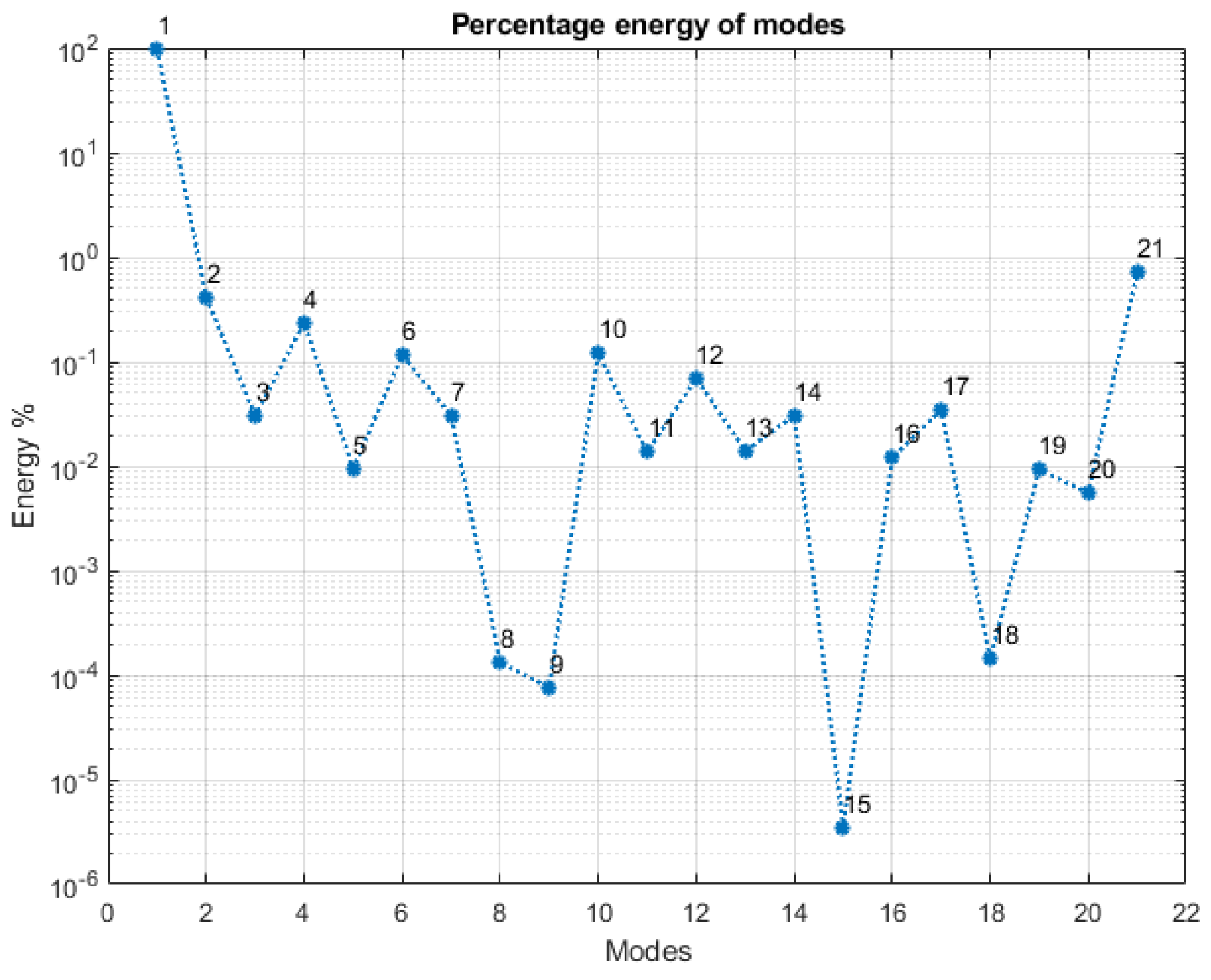
| Mode Shape | Strain energy [J] | Percent strain energy w.r.t. the total strain energy [%] |
| 1 | 14.7 | 98.1 |
| 2 | 0.0619 | 0.412 |
| Residual vector | 0.1068 | 0.712 |
| Tot | 14.9 | 99.27 |
| Ko | MM | |||
|---|---|---|---|---|
| Line 1 | Line 2 | Mode shapes 1st and 2nd (residual vector omitted) | Mode shapes 1st, 2nd and residual vector | |
| 11.07 | 10.31 | 1.434 | 1.334 | |
| 20.13 | 12.05 | 13.19 | ||
| Used Mode Shapes | Percent Strain Energy Represented w.r.t. the Total Strain Energy [%] | |
|---|---|---|
| 2:17 | 1.13 | 51.71 |
| 1 | 98.14 | 1.924 |
| 1:5 | 98.83 | 3.408 |
| 1:15 | 99.23 | 3.319 |
| 1, 2, 21 | 99.27 | 1.334 |
| 1:3, 21 | 99.30 | 1.450 |
| 1:5, 21 | 99.54 | 2.169 |
Publisher’s Note: MDPI stays neutral with regard to jurisdictional claims in published maps and institutional affiliations. |
© 2022 by the authors. Licensee MDPI, Basel, Switzerland. This article is an open access article distributed under the terms and conditions of the Creative Commons Attribution (CC BY) license (https://creativecommons.org/licenses/by/4.0/).
Share and Cite
Valoriani, F.; Esposito, M.; Gherlone, M. Shape Sensing for an UAV Composite Half-Wing: Numerical Comparison between Modal Method and Ko’s Displacement Theory. Aerospace 2022, 9, 509. https://doi.org/10.3390/aerospace9090509
Valoriani F, Esposito M, Gherlone M. Shape Sensing for an UAV Composite Half-Wing: Numerical Comparison between Modal Method and Ko’s Displacement Theory. Aerospace. 2022; 9(9):509. https://doi.org/10.3390/aerospace9090509
Chicago/Turabian StyleValoriani, Filippo, Marco Esposito, and Marco Gherlone. 2022. "Shape Sensing for an UAV Composite Half-Wing: Numerical Comparison between Modal Method and Ko’s Displacement Theory" Aerospace 9, no. 9: 509. https://doi.org/10.3390/aerospace9090509
APA StyleValoriani, F., Esposito, M., & Gherlone, M. (2022). Shape Sensing for an UAV Composite Half-Wing: Numerical Comparison between Modal Method and Ko’s Displacement Theory. Aerospace, 9(9), 509. https://doi.org/10.3390/aerospace9090509