
Surrogate-Based Optimization Design for Air-Launched Vehicle Using Iterative Terminal Guidance


Abstract
:1. Introduction
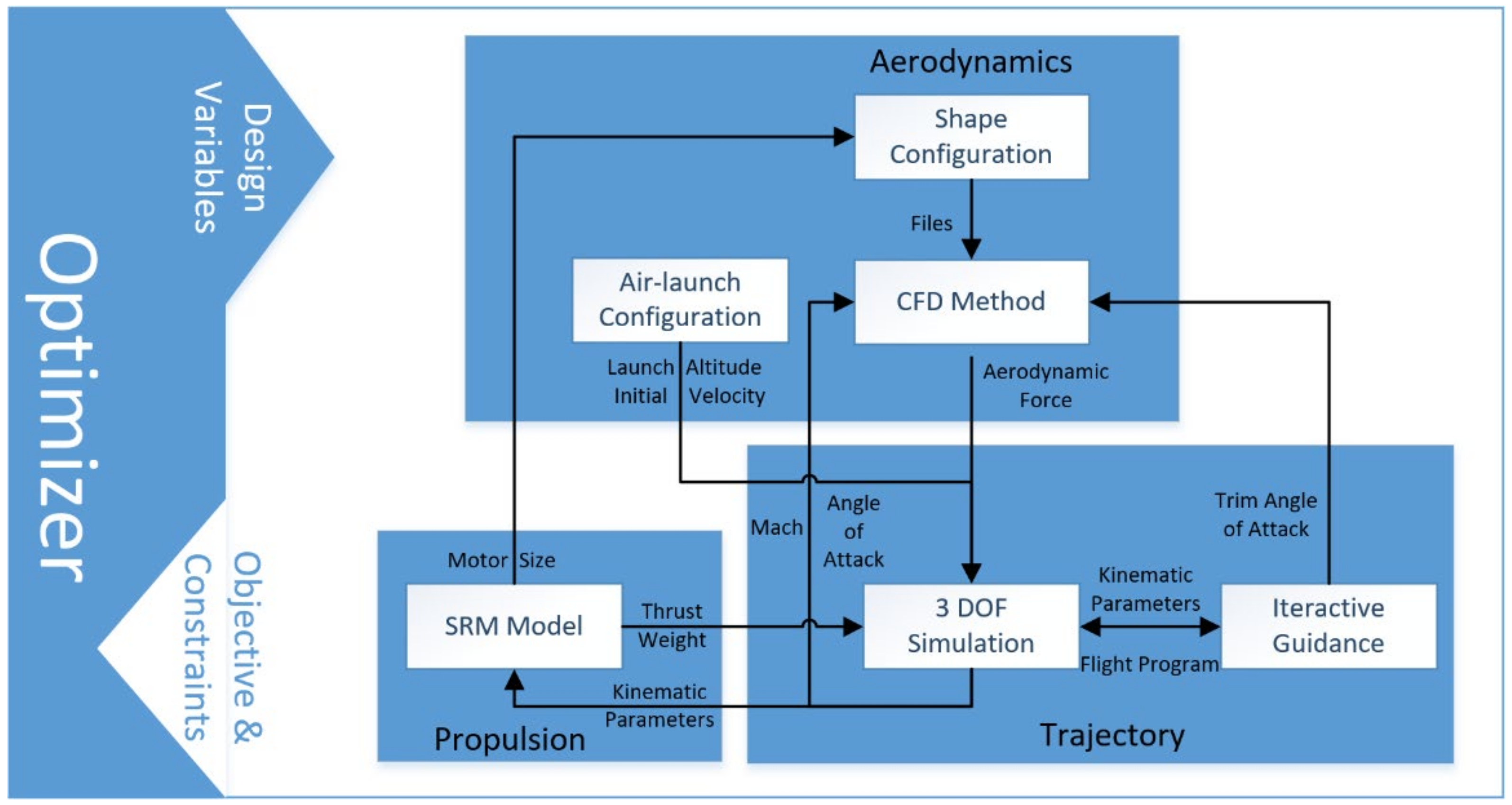
2. Multidisciplinary Optimization Framework and Overall Parameters Modules
2.1. Aerodynamic Calculation Model
2.2. Mass Estimate Module
2.3. Propulsion Module
2.4. Trajectory Module
2.5. Terminal Guidance Module
3. Optimization Design for Overall Parameters of Air-Launched Vehicle
3.1. Design Variables
3.2. Objective Function
3.3. Constraints
4. Surrogate-Based SAO Method
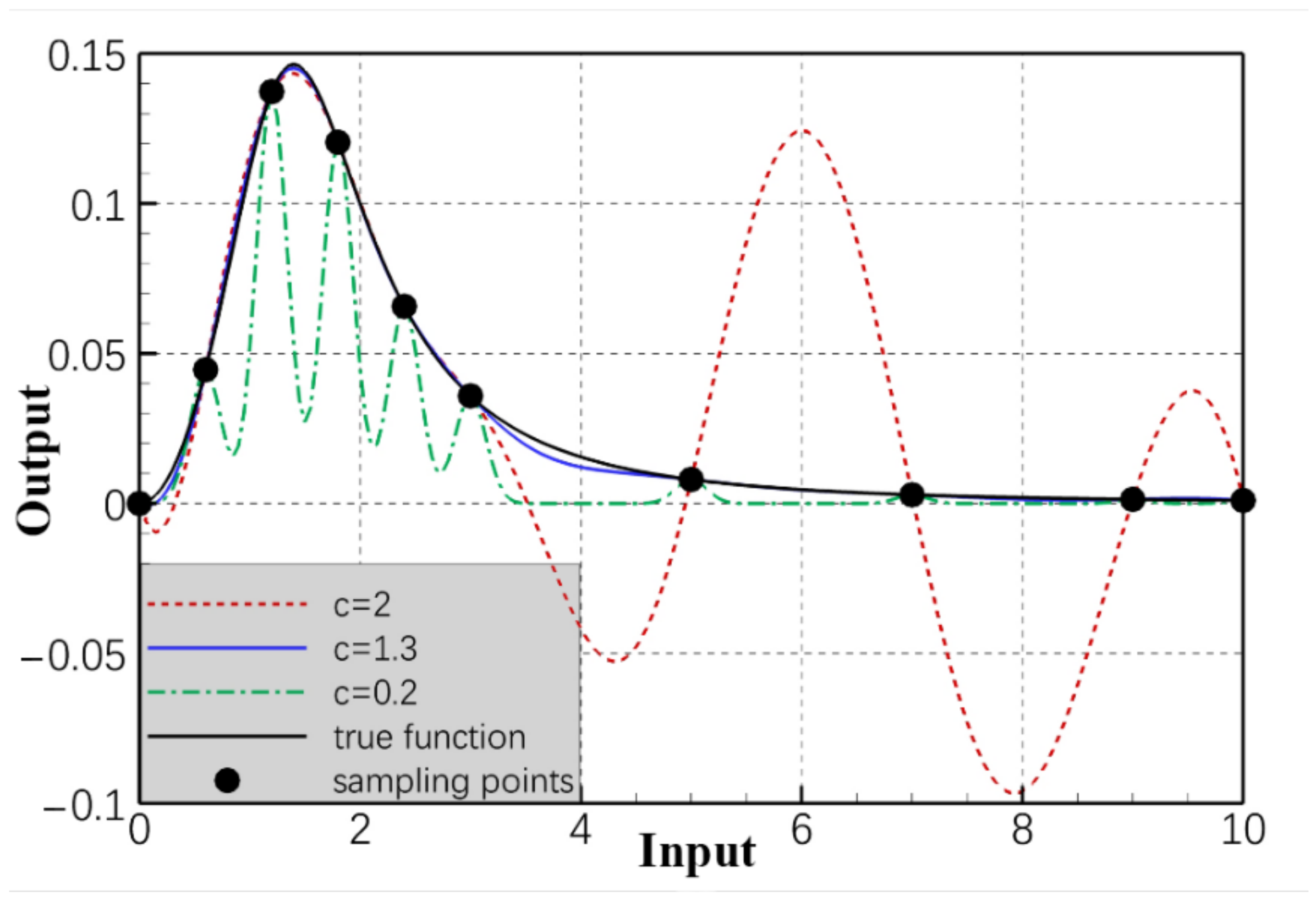
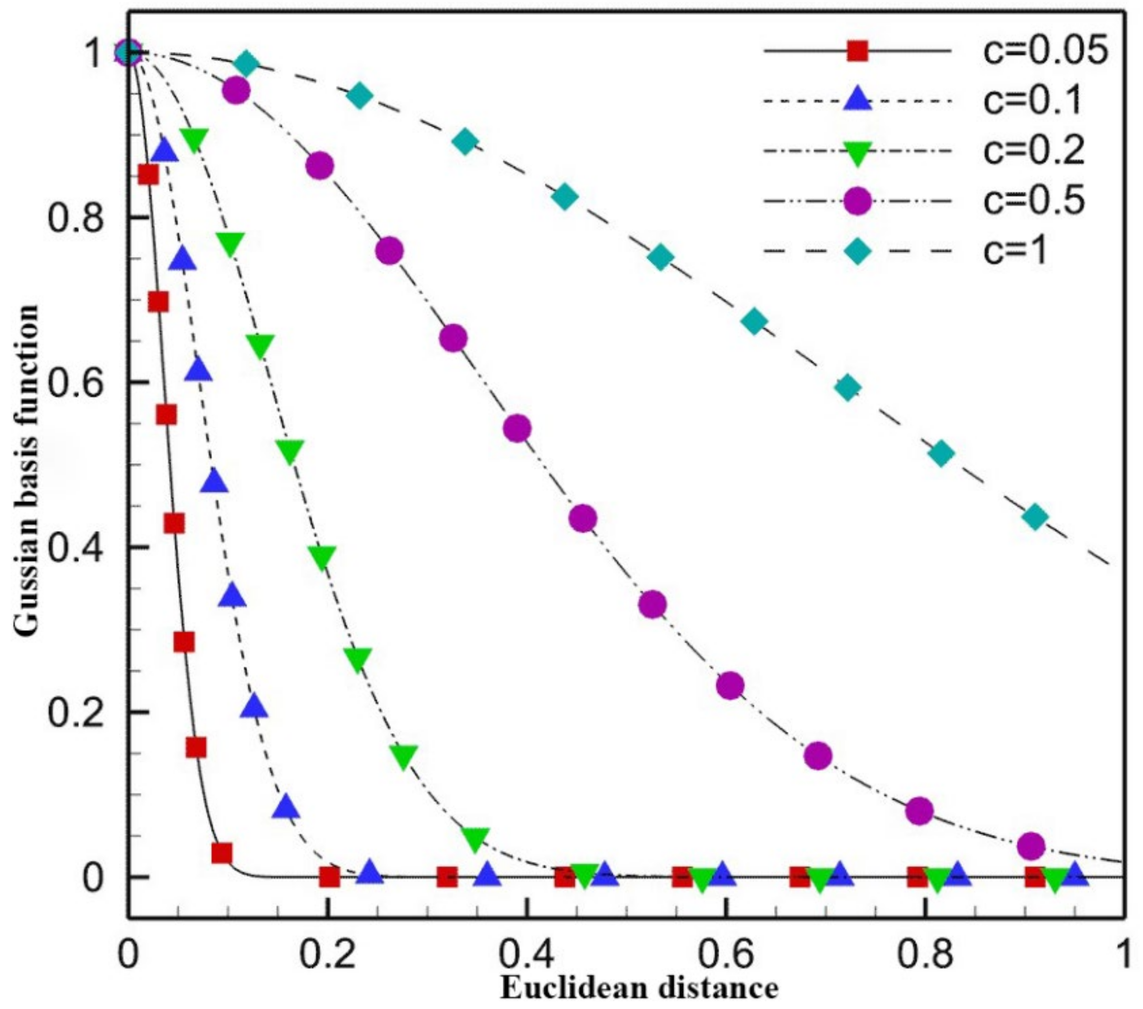
4.1. Local Density-Based RBF Shape Parameter Determination Method
4.2. Particle Swarm Optimization Method Using Adaptive Control Parameters
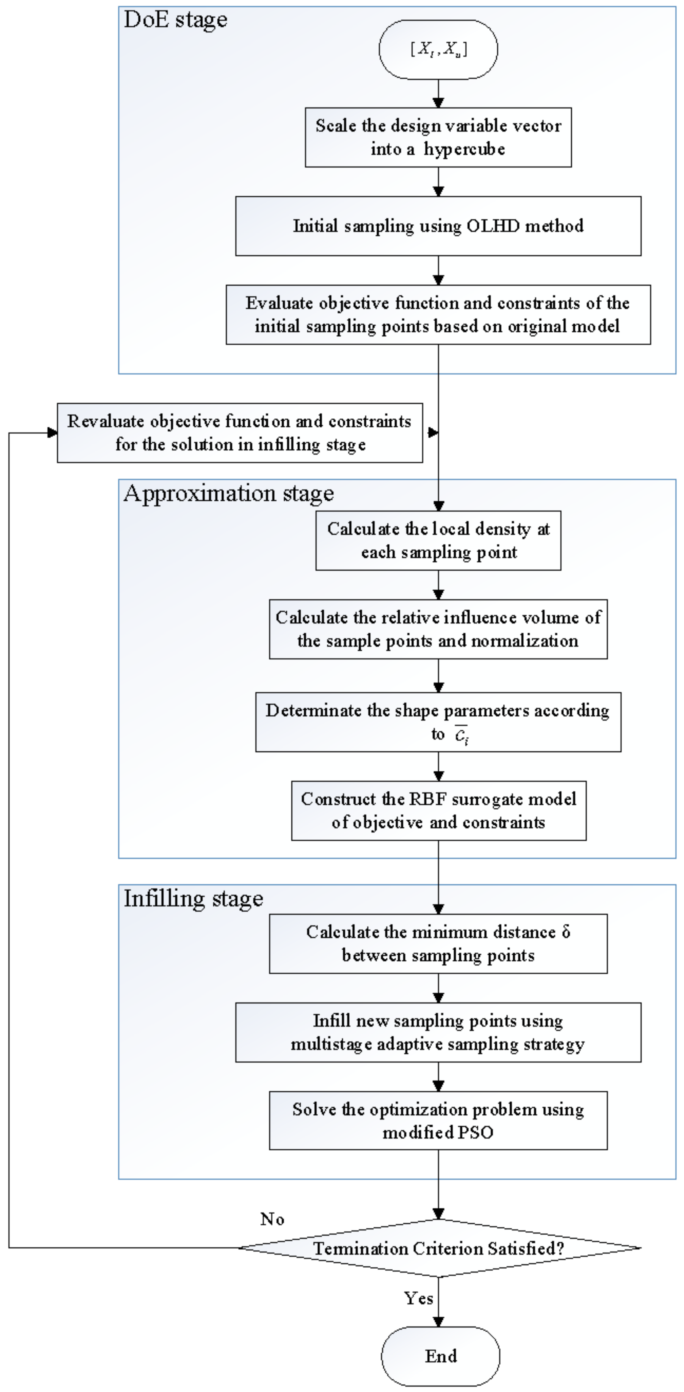
4.3. Modified Sequence Approximate Optimization Method
4.3.1. DoE Stage
4.3.2. Approximation Stage
4.3.3. Termination Criteria
4.3.4. Infilling Stage
- (1)
- Potentially feasible region locating stage (Stage 1)
- (2)
- Exploring in potentially feasible regions stage (Stage 2)
- (3)
- Optimum point of the response surfaces sampling stage (Stage 3)
4.4. Numerical Examples
5. Optimization Results and Analysis
5.1. Results and Discussion
5.2. Performance Analysis
6. Conclusions
Author Contributions
Funding
Institutional Review Board Statement
Informed Consent Statement
Data Availability Statement
Conflicts of Interest
References
- Charania, A.C.; Isakowitz, S.; Matsumori, B.; Pomerantz, W.; Vaughn, M.; Kubiak, H.; Caponio, D. LauncherOne: Virgin Galactic’s Dedicated Launch Vehicle for Small Satellites. In Proceedings of the LauncherOne: Virgin Galactics Dedicated Launch Vehicle for Small, 30th Annual AIAA/USU, Logan, UT, USA, 6–11 August 2016. [Google Scholar]
- Jiu Xing, Z.; Haojun, X.; Dengcheng, Z.; Yanhua, Z. Study on conditions of internally carried air-launched launch vehicles based on the virtual prototype technology. High Tech. Commun. 2014, 20, 166–172. [Google Scholar]
- Sarigul-Klijn, N.; Sarigul-Klijn, M. A comparative analysis of methods for air-launching vehicles from earth to sub-orbit or orbit. Proc. Inst. Mech. Eng. Part G J. Aerosp. Eng. 2006, 220, 439–452. [Google Scholar] [CrossRef]
- Lepore, D.F.; Padavano, J. AirLaunch’s QuickReach Small Launch Vehicle: Operationally Responsive Access to Space. In Proceedings of the 20th Annual AIAA/USU Conference on Small Satellites, Logan, UT, USA, 14–17 August 2006. [Google Scholar]
- Hudson, G.C. An Air-Launched Low-Cost Launch Vehicle. Am. Inst. Phys. 2005, 746, 213–219. [Google Scholar]
- Donahue, B.B. Beating the Rocket Equation: Air Launch with Advanced Chemical Propulsion. J. Spacecr. Rocket. 2004, 41, 302–309. [Google Scholar] [CrossRef]
- Rhee, I.; Lee, C.; Lee, J.-W. Optimal design for hybrid rocket engine for air launch vehicle. J. Mech. Sci. Technol. 2008, 22, 1576–1585. [Google Scholar] [CrossRef]
- Sohier, H.; Piet-Lahanier, H.; Farges, J.L. Analysis and optimization of an air-launch-to-orbit separation. Acta Astronaut. 2015, 108, 18–29. [Google Scholar] [CrossRef]
- Rafique, A.F.; He, L.S.; Zeeshan, Q.; Kamran, A.; Nisar, K. Multidisciplinary design and optimization of an air launched satellite launch vehicle using a hybrid heuristic search algorithm. Eng. Optim. 2011, 43, 305–328. [Google Scholar] [CrossRef]
- Rafique, A.; He, L.; Kamran, A.; Zeeshan, Q. Multidisciplinary design of air launched satellite launch vehicle: Performance comparison of heuristic optimization methods. Acta Astronaut. 2010, 67, 826–844. [Google Scholar] [CrossRef]
- Zhang, D.; Zhang, Y. Multidisciplinary design and optimization of an innovative nano air launch vehicle with a twin-fuselage UAV as carrier aircraft. Acta Astronaut. 2020, 170, 397–411. [Google Scholar] [CrossRef]
- Abaza, A.; Elsehiemy, R.A.; Mahmoud, K.; Lehtonen, M.; Darwish, M. Optimal Estimation of Proton Exchange Membrane Fuel Cells Parameter Based on Coyote Optimization Algorithm. Appl. Sci. 2021, 11, 2052. [Google Scholar] [CrossRef]
- Elsisi, M.; Tran, M.Q.; Hasanien, H.M.; Turky, R.A.; Albalawi, F.; Ghoneim, S.M. Robust Model Predictive Control Paradigm for Automatic Voltage Regulators against Uncertainty Based on Optimization Algorithms. Mathematics 2021, 9, 2885. [Google Scholar] [CrossRef]
- Ghoneim, S.; Mahmoud, K.; Lehtonen, M.; Darwish, M. Enhancing Diagnostic Accuracy of Transformer Faults Using Teaching-Learning Based Optimization. IEEE Access 2021, 9, 30817–30832. [Google Scholar] [CrossRef]
- Mqta, C.; Mea, D.; Mkla, B. Effective Feature Selection with Fuzzy Entropy and Similarity Classifier for Chatter Vibration Diagnosis. Measurement 2021, 184, 109962. [Google Scholar]
- Said, M.; Shaheen, A.M.; Ginidi, A.R.; El-Sehiemy, R.A.; Darwish, M. Estimating Parameters of Photovoltaic Models Using Accurate Turbulent Flow of Water Optimizer. Processes 2021, 9, 627. [Google Scholar] [CrossRef]
- Elsisi, M.; Ebrahim, M.A. Optimal design of low computational burden model predictive control based on SSDA towards autonomous vehicle under vision dynamics. Int. J. Intell. Syst. 2021, 36, 6968–6987. [Google Scholar] [CrossRef]
- Wang, D.; Wu, Z.; Fei, Y.; Zhang, W. Structural design employing a sequential approximation optimization approach. Comput. Struct. 2014, 134, 75–87. [Google Scholar] [CrossRef]
- Goldberg, D. Genetic Algorithms in Search, Optimization, and Machine Learning; Addison-Wesley Longman Publishing Co., Inc.: Boston, MA, USA, 1988; Volume 9, pp. 95–99. [Google Scholar]
- Kirkpatrick, S.; Gelatt, C.D.; Vecchi, A. Optimization by Simulated Annealing. Science 1983, 220, 671–680. [Google Scholar] [CrossRef]
- Kennedy, J.; Eberhart, R. Particle Swarm Optimization. In Proceedings of the ICNN’95—International Conference on Neural Networks, Perth, WA, Australia, 27 November–1 December 1995. [Google Scholar]
- Yıldız, A.R.Z. An effective hybrid immune-hill climbing optimization approach for solving design and manufacturing optimization problems in industry. J. Mater. Process. Technol. 2009, 209, 2773–2780. [Google Scholar] [CrossRef]
- Karaboga, D.; Basturk, B. A powerful and efficient algorithm for numerical function optimization: Artificial bee colony (ABC) algorithm. J. Glob. Optim. 2007, 39, 459–471. [Google Scholar] [CrossRef]
- Kitayama, S.; Arakawa, M.; Yamazaki, K. Sequential Approximate Optimization using Radial Basis Function network for engineering optimization. Optim. Eng. 2011, 12, 535–557. [Google Scholar] [CrossRef] [Green Version]
- Wang, G.G.; Shan, S. Review of Metamodeling Techniques in Support of Engineering Design Optimization. J. Mech. Des. 2007, 129, 415–426. [Google Scholar] [CrossRef]
- Haykin, S. Neural Networks: A Comprehensive Foundation, 3rd ed.; Prentice Hall: Hoboken, NJ, USA, 1998. [Google Scholar]
- Martin, J.D.; Simpson, T.W. Use of Kriging Models to Approximate Deterministic Computer Models. AIAA J. 2004, 43, 853–863. [Google Scholar] [CrossRef]
- Huang, D.; Allen, T.T.; Notz, W.I.; Zeng, N. Global Optimization of Stochastic Black-Box Systems via Sequential Kriging Meta-Models. J. Glob. Optim. 2006, 34, 441–466. [Google Scholar] [CrossRef] [Green Version]
- Kleijnen, J. Kriging metamodeling in simulation: A review. Eur. J. Oper. Res. 2009, 192, 707–716. [Google Scholar] [CrossRef] [Green Version]
- Buhmann, M. Radial Basis Functions. Scholarpedia 2010, 5, 9837. [Google Scholar] [CrossRef]
- Schwenker, F.; Kestler, H.A.; Palm, G. Three learning phases for radial-basis-function networks. Neural Netw. 2001, 14, 439–458. [Google Scholar] [CrossRef]
- Park, J.; Sandberg, I. Universal Approximation Using Radial-Basis-Function Networks. Neural Comput. 2014, 3, 246–257. [Google Scholar] [CrossRef]
- Basak, D.; Srimanta, P.; Patranbis, D.C. Support Vector Regression. Neural Inf. Process. Lett. Rev. 2007, 11, 203–224. [Google Scholar]
- Suykens, J.A.K.; Brabanter, J.D.; Lukas, L.; Vandewalle, J. Weighted least squares support vector machines: Robustness and sparse approximation. Neurocomputing 2002, 48, 85–105. [Google Scholar] [CrossRef]
- Evgeniou, T.; Pontil, M.; Poggio, T. Regularization Networks and Support Vector Machines. Adv. Comput. Math. 2000, 13, 1–50. [Google Scholar] [CrossRef]
- Unal, R.; Lepsch, R.; Engelund, W.; Stanley, D. Approximation model building and multidisciplinary design optimization using response surface methods. In Proceedings of the Symposium on Multidisciplinary Analysis & Optimization, Bellevue, WA, USA, 4–6 September 1996. [Google Scholar]
- Venter, G.; Haftka, R.T.; Starnes, J.H. Construction of Response Surfaces for Design Optimization Applications. In Proceedings of the 6th AIAA/NASA/ISSMO Symposium on Multidisciplinary Analysis & Optimization, Bellevue, WA, USA, 4–6 September 1996. [Google Scholar]
- Chen, W.; Allen, J.K.; Mavris, D. A concept exploration method for determining robust top-level specifications. Eng. Optim. 1996, 26, 137–158. [Google Scholar] [CrossRef]
- Hardy, R.L. Multiquadric equations of topography and other irregular surfaces. J. Geophys. Res. 1971, 76, 1905–1915. [Google Scholar] [CrossRef]
- Jin, R.; Chen, W.; Simpson, T.W. Comparative Studies of Metamodeling Techniques under Multiple Modeling Criteria. J. Struct. Multidiscip. Optim. 2001, 23, 1–13. [Google Scholar] [CrossRef]
- Han, H.; Wu, X.; Zhang, L.; Tian, Y.; Qiao, J. Self-Organizing RBF Neural Network Using an Adaptive Gradient Multi-objective Particle Swarm Optimization. IEEE Trans. Cybern. 2017, 49, 69–82. [Google Scholar] [CrossRef]
- Zhang, Y.; Gong, C.; Fang, H.; Su, H.; Li, C.; Da Ronch, A. An efficient space-division-based width optimization method for RBF network using fuzzy clustering algorithms. Struct. Multidiscip. Optim. 2019, 60, 461–480. [Google Scholar] [CrossRef] [Green Version]
- Fei, L.; Yang, C.; Qiao, J. A novel RBF neural network design based on immune algorithm system. In Proceedings of the 2017 36th Chinese Control Conference (CCC), Dalian, China, 26–28 July 2017. [Google Scholar]
- Slema, S.; Errachdi, A.; Benrejeb, M. A Radial Basis Function Neural Network Model Reference Adaptive Controller for Nonlinear Systems. In Proceedings of the 2018 15th International Multi-Conference on Systems, Signals & Devices (SSD), Yasmine Hammamet, Tunisia, 19–22 March 2018. [Google Scholar]
- Wang, D.; Fan, H.; Ma, Z.; Wu, Z.; Zhang, W. A CAD/CAE integrated framework for structural design optimization using sequential approximation optimization. Adv. Eng. Softw. 2014, 76, 56–68. [Google Scholar] [CrossRef]
- Chen, K.; Liu, L.; Meng, Y. Launch Vehicle Flight Dynamics and Guidance; National Defense Industry Press: Beijing, China, 2014. [Google Scholar]
- Zhao, Y.; Sheng, Y.; Liu, X. Sliding mode control based guidance law with impact angle constraint. Chin. J. Aeronaut. 2014, 27, 145–152. [Google Scholar] [CrossRef] [Green Version]
- Chen, K.; Zhou, F.; Yin, L.; Wang, S.; Wang, Y.; Wan, F. A hybrid particle swarm optimizer with sine cosine acceleration coefficients. Inf. Sci. 2017, 422, 218–241. [Google Scholar] [CrossRef]
- Li, J.; Peng, K.; Wang, W.; Wu, Z.; Zhang, W. Optimization design of rockoons based on improved sequential approximation optimization. Proc. Inst. Mech. Eng. Part G J. Aerosp. Eng. 2022, 236, 140–153. [Google Scholar] [CrossRef]
- Dong, H.; Song, B.; Wang, P.; Dong, Z. Surrogate-based optimization with clustering-based space exploration for expensive multimodal problems. Struct. Multidiscip. Optim. 2018, 57, 1553–1577. [Google Scholar] [CrossRef]
- Jones, D.R.; Schonlau, M.; Welch, W.J. Efficient Global Optimization of Expensive Black-Box Functions. J. Glob. Optim. 1998, 13, 455–492. [Google Scholar] [CrossRef]
- Gu, J.; Li, G.Y.; Dong, Z. Hybrid and adaptive meta-model-based global optimization. Eng. Optim. 2012, 44, 87–104. [Google Scholar] [CrossRef]


| Overall Parameters | Three Stage Case | Four Stage Case |
|---|---|---|
| Specific impulse (m/s) | = 2450 = = 2750 | = 2450 = = = 2750 |
| Average thrust (kN) | = 800 = 123 = 18 | = 800 = 450 = 120 = 18 |
| Propellant mass ratio | 1st: 0.93 2nd: 0.92 3rd: 0.89 | 1st: 0.93 2nd: 0.92 3rd: 0.89 4th: 0.85 |
| Objective orbit | 500 km SSO | |
| Launch altitude (km) | 10.67 | |
| Initial velocity (m/s) | 262 | |
| Launch velocity inclination (°) | 25 | |
| Takeoff mass (ton) | 25.85 | |
| Payload mass (kg) | 300 | |
| Total length (m) | 21.34 | |
| Design Variables (Units) | Description | 3-Stage Configuration | 4-Stage Configuration | ||
|---|---|---|---|---|---|
| Lower Limit | Upper Limit | Lower Limit | Upper Limit | ||
| (kN) | Average thrust of 1st stage motor | 600 | 1000 | 800 | 1200 |
| (s) | Working time of 1st stage motor | 40 | 60 | 40 | 80 |
| (kN) | Average thrust of 1st stage motor | 50 | 500 | 400 | 800 |
| (s) | Working time of 1st stage motor | 30 | 55 | 30 | 60 |
| (kN) | Average thrust of 1st stage motor | 18 | 100 | 100 | 300 |
| (s) | Working time of 1st stage motor | 10 | 30 | 20 | 40 |
| (kN) | Average thrust of 1st stage motor | -- | -- | 20 | 40 |
| (s) | Working time of 1st stage motor | -- | -- | 10 | 35 |
| (s) | Gliding time of 1st stage | 15 | 30 | 15 | 30 |
| (s) | Gliding time of 2nd stage | 200 s | 500 | 100 | 300 |
| (s) | Gliding time of 3rd stage | -- | -- | 200 | 500 |
| (kg) | Mass of the payload | −300 | 300 | −500 | 500 |
| (s) | Working time of program angle | 5 | 40 | 20 | 50 |
| (deg) | Program angle of attack | 0.5 | 20 | 0.5 | 20 |
| Benchmark Function | Number of Design Variables | Design Space | Global Optimum |
|---|---|---|---|
| 2 | [−2,2] | −186.7309 | |
| 6 | [0,1] | −3.32 | |
| 2 | [−5,10] | 0 | |
| 2 | [−10,10] | 0 | |
| 10 | [−600,600] | 0 |
| Functions | ||||||
|---|---|---|---|---|---|---|
| SAO | Best | −186.728 | −3.319 | 2.84 × 10⁷ | 1.87 × 10⁶ | 3.36 × 10³ |
| Median | −186.717 | −3.313 | 1.93 × 10⁴ | 5.90 × 10⁵ | 4.25 × 10² | |
| Worst | −185.055 | −3.300 | 3.08 × 10³ | 7.57 × 10³ | 9.56 × 10² | |
| MNFE | 48 | 49 | 54 | 67 | >300 | |
| SOCE | Best | −186.701 | −3.317 | 7.58 × 10⁶ | 2.86 × 10⁶ | 1.18 × 10² |
| Median | −186.053 | −3.306 | 2.72 × 10⁴ | 2.14 × 10⁴ | 3.28 × 10² | |
| Worst | −185.342 | −3.290 | 8.47 × 10⁴ | 8.28 × 10⁴ | 9.75 × 10² | |
| MNFE | 68 | 89 | 135 | 140 | >300 | |
| KMS | Best | −186.203 | −3.312 | 2.32 × 10⁵ | 7.40 × 10³ | 0.912 |
| Median | −101.456 | −3.308 | 5.04 × 10⁴ | 8.63 × 10³ | 1.093 | |
| Worst | −39.589 | −3.291 | 2.80 × 10³ | 1.97 × 10² | 1.367 | |
| MNFE | >244 | 87 | >198 | >300 | >300 | |
| EGO | Best | −186.664 | −3.318 | 6.31 × 10⁶ | 1.03 × 10⁶ | 13.968 |
| Median | −186.109 | −3.298 | 7.68 × 10⁴ | 5.73 × 10⁴ | 28.083 | |
| Worst | −184.941 | −3.201 | 7.71 × 10³ | 3.53 × 10³ | 56.223 | |
| MNFE | 71 | >123 | >158 | >157 | >300 | |
| HAM | Best | −186.720 | −3.316 | 3.31 × 10⁶ | 2.30 × 10⁶ | 9.88 × 10³ |
| Median | −119.826 | −3.295 | 7.51 × 10⁵ | 7.40 × 10³ | 2.39 × 10² | |
| Worst | −39.589 | −3.159 | 2.35 × 10⁴ | 9.86 × 10³ | 0.585 | |
| MNFE | 209 | >151 | 48 | >244 | >300 | |
| Cases | Configuration | Optimization Method | Terminal Guidance |
|---|---|---|---|
| Case1 | 3 stages | PSO | None |
| Case2 | Employ | ||
| Case3 | SAO | None | |
| Case4 | Employ | ||
| Case5 | 4 stages | PSO | None |
| Case6 | Employ | ||
| Case7 | SAO | None | |
| Case8 | Employ |
| Variables | Case 1 | Case 2 | Case 3 | Case 4 | Case 5 | Case 6 | Case 7 | Case 8 |
|---|---|---|---|---|---|---|---|---|
| (kN) | 993.01 | 777.27 | 898.52 | 765.26 | 811.28 | 846.44 | 909.97 | 878.58 |
| (s) | 47.68 | 54.72 | 44.46 | 54.39 | 47.19 | 45.79 | 42.75 | 42.41 |
| (kN) | 226.88 | 441.03 | 383.20 | 482.45 | 552.66 | 479.55 | 409.94 | 414.07 |
| (s) | 39.58 | 30.90 | 42.12 | 30.03 | 31.93 | 36.10 | 40.70 | 42.05 |
| (kN) | 46.42 | 80.62 | 60.11 | 45.80 | 144.20 | 110.68 | 128.40 | 135.38 |
| (s) | 31.00 | 25.00 | 41.93 | 49.29 | 17.90 | 18.62 | 19.16 | 24.37 |
| (kN) | -- | -- | -- | -- | 25.04 | 37.55 | 39.74 | 42.45 |
| (s) | -- | -- | -- | -- | 24.88 | 21.50 | 26.02 | 29.51 |
| (s) | 15.47 | 16.16 | 25.12 | 26.58 | 20.19 | 15.28 | 29.90 | 16.25 |
| (s) | 456.17 | 410.75 | 380.63 | 396.13 | 222.94 | 113.66 | 89.69 | 96.10 |
| (s) | -- | -- | -- | -- | 349.67 | 469.39 | 421.88 | 373.18 |
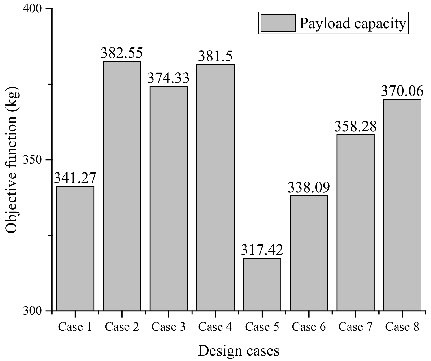
| (kg) | 341.27 | 382.55 | 374.33 | 381.50 | 317.42 | 338.09 | 358.28 | 370.06 |
| (s) | 12.71 | 22.09 | 24.21 | 18.04 | 44.84 | 49.09 | 18.75 | 76.66 |
| (deg) | 10.10 | 14.30 | 12.03 | 19.13 | 8.26 | 5.63 | 13.36 | 6.00 |
Publisher’s Note: MDPI stays neutral with regard to jurisdictional claims in published maps and institutional affiliations. |
© 2022 by the authors. Licensee MDPI, Basel, Switzerland. This article is an open access article distributed under the terms and conditions of the Creative Commons Attribution (CC BY) license (https://creativecommons.org/licenses/by/4.0/).
Share and Cite
Li, J.; Wang, D.; Zhang, W. Surrogate-Based Optimization Design for Air-Launched Vehicle Using Iterative Terminal Guidance. Aerospace 2022, 9, 300. https://doi.org/10.3390/aerospace9060300
Li J, Wang D, Zhang W. Surrogate-Based Optimization Design for Air-Launched Vehicle Using Iterative Terminal Guidance. Aerospace. 2022; 9(6):300. https://doi.org/10.3390/aerospace9060300
Chicago/Turabian StyleLi, Jiaxin, Donghui Wang, and Weihua Zhang. 2022. "Surrogate-Based Optimization Design for Air-Launched Vehicle Using Iterative Terminal Guidance" Aerospace 9, no. 6: 300. https://doi.org/10.3390/aerospace9060300
APA StyleLi, J., Wang, D., & Zhang, W. (2022). Surrogate-Based Optimization Design for Air-Launched Vehicle Using Iterative Terminal Guidance. Aerospace, 9(6), 300. https://doi.org/10.3390/aerospace9060300