Effects of Surface Errors of Antennas on Detection Performance of Space VLBI

Abstract

This work investigates the effects of the surface errors of the satellite antenna on the detection performance of the space VLBI system. First, the relationship between the surface errors and the antenna gain loss is analyzed, and then the influence of the gain loss on the detection performance of the VLBI system is analyzed. Both the uniform and nonuniform distributions of errors are studied, and the second-order Taylor expansion is performed on the errors to simplify the calculation. When the errors distribute nonuniformly, the solver SCIP is adopted to solve the corresponding distribution, which leads to the maximum gain loss of the antenna. Taking the VLBI system with two base stations as the object, and each station’s radio telescope is a hoop truss deployable antenna with 30 m aperture, the effects of antenna gain loss on the detection capability of the radio telescope and the delay error of the VLBI system are studied. The study of extreme working conditions will have a higher guiding significance for the overall link analysis of practical projects.

1. Introduction

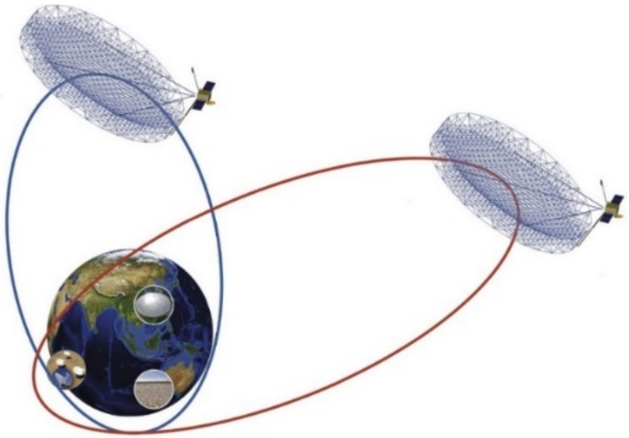
Very long baseline interferometry (VLBI) is an astronomical observation technique with the highest spatial resolution and has been widely used in deep space exploration [1]. The resolution of VLBI is proportional to its baseline length and observation frequency, as shown in Figure 1. In the case of a certain wavelength, in order to obtain a higher resolution, it is necessary to launch some radio telescopes into space to form a space VLBI network (SVLBI) [2]. The baseline length of the SVLBI is much larger than the diameter of the earth, as shown in Figure 2. Limited by the size of the rocket launch envelope, it is necessary to use a deployable space antenna in order to obtain a sufficiently high antenna gain. The truss-type deployable antenna is one of the most widely used types of space satellite antennas, and can meet the requirements of a good flexibility, light weight, high surface accuracy and high stability [3].

Figure 1. Schematic diagram of very long baseline interferometry. d is the distance between the two antennas, $\theta$ is the signal source direction and $\tau$ is the geometric delay characterizing the time difference between the arrival of the signal to the two antennas.

Figure 2. Sketch of SVLBI.

In order to ensure a high electromagnetic performance, antennas have high requirements for the accuracy of the reflector surface [4], and the root-mean-square error (rms) is a standard parameter used to characterize random surface errors. Paolo Rocca [5] divided the root-mean-square of the surface errors into a certain number of areas for radiation analysis, and then integrated the entire aperture surface to obtain the total antenna radiation, which is an effective method when the errors distribute uniformly. In order to analyze the electrical performance deeper when the surface errors distribute nonuniformly, Peiyuan Lian [6] used a genetic algorithm to analyze the antenna gain loss and the first side lobe level under the nonuniform distribution. However, the disadvantage is that the obtained result may not be the global optimal solution.

Then, under the premise of meeting the accuracy requirements, scholars applied the Taylor expansion to approximate the influence of antenna error analysis to further reduce the complexity of mathematical operations; the resulting approximate radiation integral is then decomposed by expanding an exponential phase error function. Abolfazl Haddadi [7] analyzed the radiation integral using functional calculus and extracted the first variational derivative of the radiation field of the surface profile. Shuxin Zhang [8] applied the second-order Taylor expansion to the phase error analysis caused by the parabolic antenna profile error. Compared with the conventional method, the deviation can be ignored. Although the antenna performance when the errors are not uniformly distributed has been studied in [8], this paper will further study the case where the gain loss is maximized.

Different from the research on general radars and communication antennas, the focus of this paper is the gain loss caused by the antenna surface errors of the 30 m aperture space VLBI observatory. The antenna gain loss is further studied for its influence on the antenna’s minimum detection ability and the resolution of the VLBI system. This paper not only applies the second-order Taylor expansion to the study of the electrical performance of the antenna when the surface errors distribute nonuniformly, but also establishes a mathematical model that takes the gain loss as the objective function, where solving constraint integer programs (SCIP) can be applied when the errors distribute nonuniformly.

2. Formulation

The times for the electromagnetic waves radiated by the radio source to reach different VLBI observation stations at a certain moment are different. Take the VLBI system of two base stations as the project. Under ideal conditions, the signals $x\left(t\right)$ and $y(t+\tau )$ detected by the two base stations should be completely consistent, except for the time delay $\tau$. However, due to various interferences, the delay value that minimizes the variance of the two signals in actual processing is the required delay value, as shown in (1):

$$minQ\left(\tau \right)={\int }_{-\infty }^{+\infty }{[x\left(t\right)-y(t+\tau )]}^{2}dt$$

(1)

Expanding and simplifying can transform the problem into maximizing signal autocorrelation as

$$maxR\left(\tau \right)={\int }_{-\infty }^{+\infty }x\left(t\right)y(t+\tau )dt$$

(2)

For SVLBI, the detection error comes from various factors, such as the performance of the antenna itself, the movement of the earth, atmospheric interference and the space environment. In this study, the main concern is the performance change in the satellite antenna, so other effects are idealized. The detection accuracy under this condition depends on the sensitivity of the receiver, which means the ability to receive weak signals, usually expressed by the minimum detectable signal power. In the field of radio astronomy, the sensitivity of the antenna is usually measured by the system equivalent flux density (SEFD) as

$$f_{sys}=\frac{2k}{\eta A}{T}_s$$

(3)

where k is the Planck constant, $\eta$ is the efficiency of the antenna, A is the antenna aperture area and $T_s$ is the system noise temperature. Then, the deterioration of the minimum observable flux density $F_{min}$ of the radio telescope is computed as

$$F_{min}=\frac{2k{T}_s}{\eta A\sqrt{TB}}$$

(4)

where T is the integration time and B is the observation bandwidth. In actual engineering, $\eta$ is jointly determined by radiation efficiency $e_r$ (the ratio of the total power radiated by an antenna to the net power accepted by the antenna from the connected transmitter), sharpening efficiency ${\eta }_t$ (the antenna aperture field distribution is generally higher in the center than at the edge), overflow power ${\eta }_s$ (the power pattern of the feed always has a part outside the reflector) and technical efficiency ${\eta }_a$ (feed phase error, design error, etc.), $\eta =e_r{\eta }_t{\eta }_s{\eta }_a$.

Among them, the technical efficiency ${\eta }_a$ is determined by the antenna surface errors, aperture occlusion, feed phase errors, etc. Combined with the analysis of this article, other factors are idealized, and only the antenna profile error is concerned.

$F_{min}$ is the analysis target of a single base station antenna, and the signal-to-noise ratio (SNR) of a VLBI system is determined by the antennas of multiple base stations. For a VLBI system with two base stations,

$$SNR=\frac{2}{\pi }\sqrt{\frac{T_{a1}{T}_{a2}{N}_b}{T_{s1}{T}_{s2}}}$$

(5)

where $N_b$ is the noise bandwidth and $T_{si}(i=1,2)$ is the system noise temperature. The error of the VLBI observation index delay caused by surface shape errors can be derived from (6).

$${\sigma }_{\tau }=\frac{\sqrt{2}c}{2\pi B\sqrt{T}}\frac{1}{SNR}$$

(6)

$$T_{ai}=0.0003{\eta }_{i}A{S}_c$$

(7)

where $T_{ai}(i=1\&2)$ is the effective source temperature of the observing station, $N_b$ is the noise bandwidth, ${\eta }_i$ is the antenna efficiency and $S_c$ is the flux density of radio source.

From the above analysis, it can be seen that, after the other factors are idealized, only the influence of the shape error on the antenna efficiency needs to be studied, and the antenna gain and efficiency meet the following requirements:

$$G=\frac{4\pi A}{{\lambda }^2}\eta$$

(8)

To analyze the influence of the surface shape accuracy on the antenna gain, the radiation characteristics of the antenna with the surface shape error must be studied first. The geometry of a parabolic reflector with random surface errors is depicted in Figure 3. The aperture has a diameter $D=2a$ and a focal length F, A is the projected region on the focal plane with the polar coordinates ${\rho }^{\prime }$ and ${\varphi }^{\prime }$, and $\widehat{r}$ is the unit vector in the observation direction. Here, the amplitude aperture distribution is

$$Q\left({\rho }^{\prime }\right)=B+C{(1-\frac{{\rho }^{\prime }}{a^2})}^P$$

(9)

where B and P determine the shape of the aperture distribution, $C=1-B$, the edge taper $ET=20logB$ and, for engineering, $1\le P\le 2$.

Figure 3. Reflector with random surface errors.

The far field pattern of the antenna is proportional to the Fourier transform of its aperture distribution and may be expressed as

$$E=\int \int Q\left({\rho }^{\prime }\right)e^{j\delta }{e}^{jk{\overrightarrow{\rho }}^{\prime }·\overrightarrow{r}}d{s}^{\prime }$$

(10)

The model of [9] is adopted. It is assumed that the reflector aperture is divided into N annular regions as shown in Figure 4, where ${\rho }_n=\frac{1}{2}(a_n+a_{n-1})$, $tan{\xi }_n=\frac{{\rho }_n}{2F}$ and ${\sigma }_n=\frac{4\pi }{\lambda }{\epsilon }_{rms\left(n\right)}cos{\xi }_n$. By assuming that the phase errors ${\delta }_n$ in the $nth$ annular region and ${\delta }_m$ in the $mth$ annular region are statistically independent and have Gaussian distribution with zero mean and standard deviation equal to ${\sigma }_n$ and ${\sigma }_m$, respectively, the radiation pattern of the antenna with surface errors can be derived as

$$E=\sum _{n=1}^N{E}_{n,n-1}{e}^{j{\delta }_n}$$

(11)

where

$$E_{n,n-1}=E_n-E_{n-1}={\int }_{a_{n-1}}^{a_n}{\int }_0^{2\pi }Q\left({\rho }^{\prime }\right)e^{jk{\rho }^{\prime }\sin \theta \cos (\varphi -{\varphi }^{\prime })}{\rho }^{\prime }d{\rho }^{\prime }d{\varphi }^{\prime }$$

(12)

Figure 4. Reflector aperture divided into N annular regions.

Zhang et al. [8] have proven that the second-order Taylor expansion can not only ensure the calculation accuracy but also reduce the computational complexity. Performing the second-order Taylor series expansion on phase errors and combining the radiation fields in subdivision strips, the radiation pattern can be expressed as

$$E=\sum _{n=1}^N{E}_{n,n-1}(1+j{\delta }_n-\frac{1}{2}{\delta }_n^2)$$

(13)

The radiated power can be constructed as

$$E{E}^{\ast }=\sum _{n=1}^N{E}_{n,n-1}(1+j{\delta }_n-\frac{1}{2}{\delta }_n^2)·\sum _{m=1}^N{E}_{m,m-1}^{\ast }(1-j{\delta }_m-\frac{1}{2}{\delta }_m^2)$$

(14)

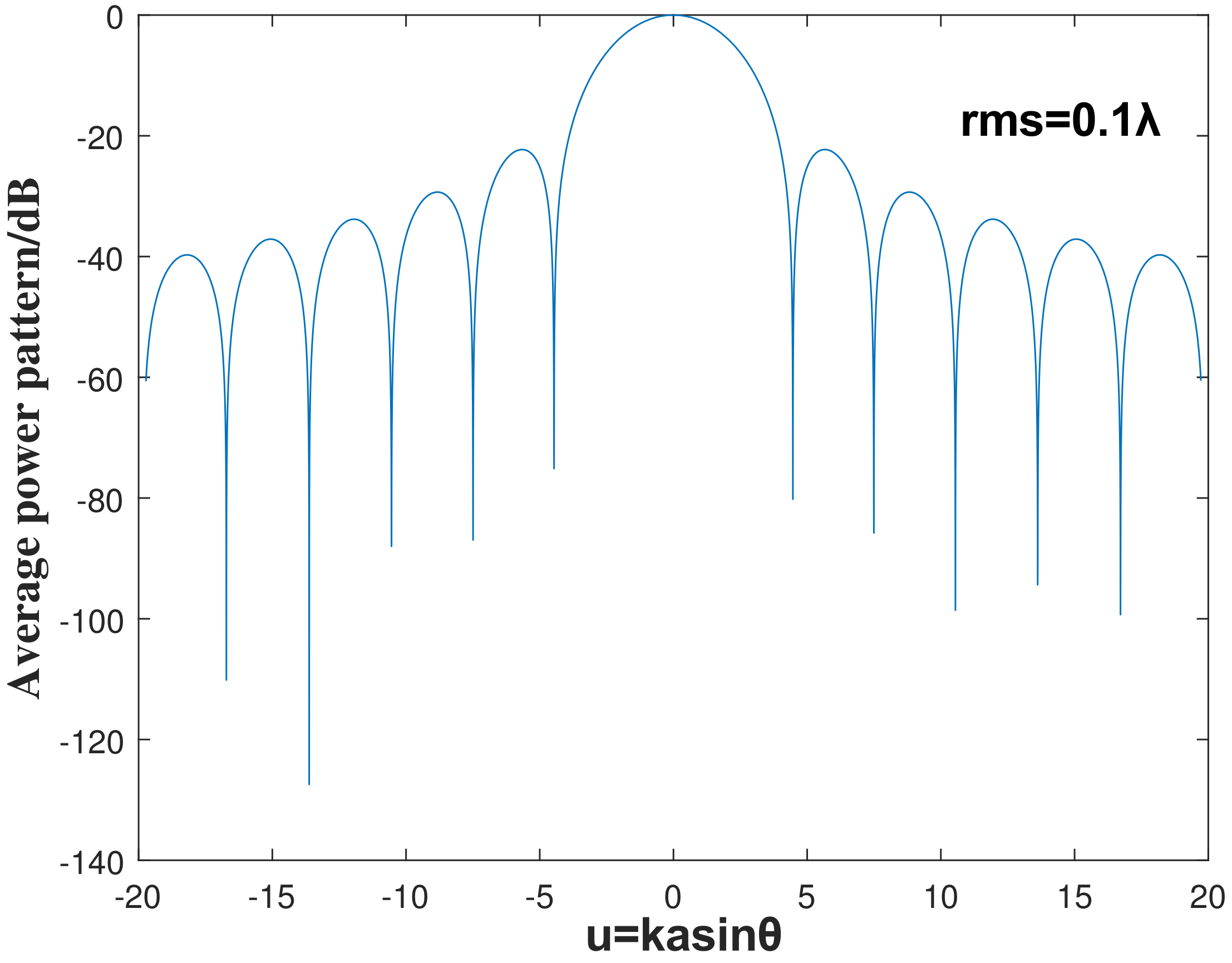
The corresponding average radiation power is

$$\overline{E{E}^{\ast }}=\sum _{n=1}^N\sum _{m=1}^N{E}_{n,n-1}{E}_{m,m-1}^{\ast }(1-\frac{1}{2}{\sigma }_n^2-\frac{1}{2}{\sigma }_m^2+\frac{1}{4}{\sigma }_n^2{\sigma }_m^2)$$

(15)

Here, the regular formula for solving $\overline{E{E}^{\ast }}$ is given in order to compare the results of subsequent experiments:

$$\overline{E{E}^{\ast }}=\sum _{n=1}^N\sum _{m=1}^N{E}_{n,n-1}{E}_{m,m-1}^{\ast }{e}^{-0.5({\sigma }_n^2+{\sigma }_m^2)}+\sum _{n=1}^N{E}_{n,n-1}{E}_{n,n-1}^{\ast }(1-{\sigma }_n^2)$$

(16)

In actual engineering, antenna designers usually use the Ruze formula to estimate the gain loss as [9] when the surface errors are uniformly distributed:

$$PGL=10log{e}^{-{(4\pi \kappa {\mathcal{E}}_{rms}/\lambda )}^2}$$

(17)

where ${\mathcal{E}}_{rms}$ is the root-mean-square value of random surface errors, is the wavelength and $\kappa$ is the correction factor.

Before proposing the analysis scheme, give the weight coefficient $S_n$ of each ring and the relationship between the root-mean-square value of each ring surface error ${\mathcal{E}}_{rms\left(n\right)}$ and the root-mean-square error of the entire reflecting surface ${\mathcal{E}}_{rms\left(n\right)}$:

$$a_n=\frac{n}{N}a$$

(18)

$$S_n=\sum _{n=1}^N\frac{a_n^2-a_{n-1}^2}{a^2}$$

(19)

$${\epsilon }_{rms}^2=\sum _{n=1}^N{S}_n{\epsilon }_{rms\left(n\right)}^2$$

(20)

The mathematical model to be established is to find the distribution of the error with the maximum gain loss of the antenna as the objective function given the ${\mathcal{E}}_{rms}$. The model is briefly shown as

$$find{\mathcal{E}}_{\mathbf{rms}}=({\epsilon }_{rms\left(1\right)},{\epsilon }_{rms\left(2\right)},\dots ,{\epsilon }_{rms\left(N\right)})$$

(21)

$$minF\left({\mathcal{E}}_{\mathbf{rms}}\right)=\left(antennagain\right)$$

(22)

s.t.

$$\sum _{n=1}^N{S}_n{\epsilon }_{rms\left(n\right)}^2={\epsilon }_{rms}^2(n=1,2,\dots ,N)$$

(23)

$$0\le {\epsilon }_{rms\left(n\right)}^2\le {\epsilon }_{rms}^2/S_n$$

(24)

As for the mathematical model where the error is only distributed in a single circle, its constraint becomes much simpler:

$${\epsilon }_{rms\left(n\right)}^2={\epsilon }_{rms}^2/S_n(n=1,2,\dots ,N)$$

(25)

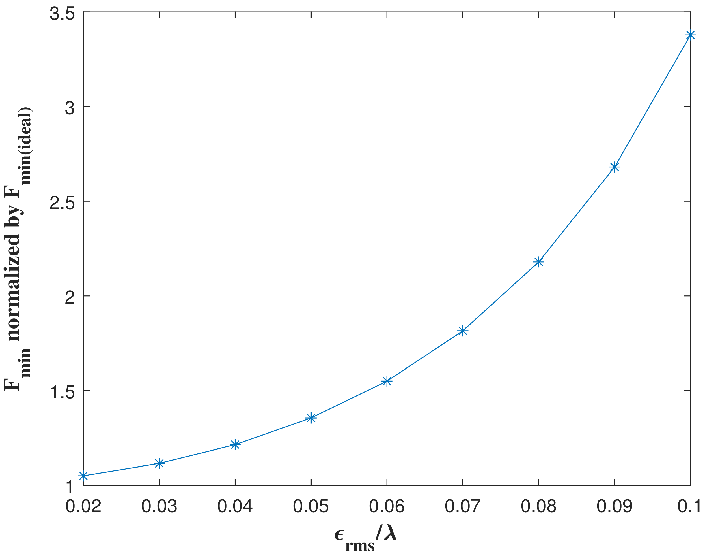
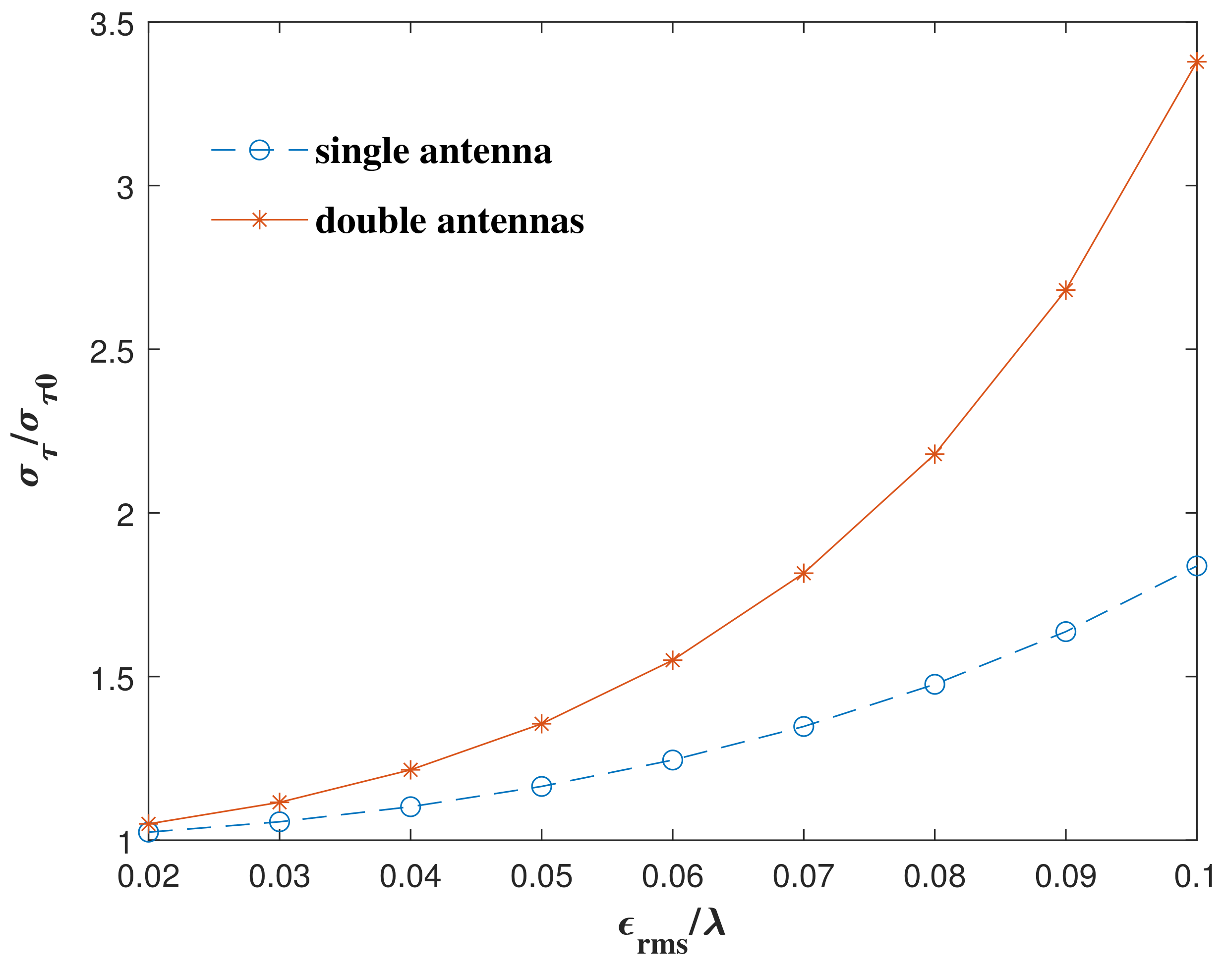
As mentioned earlier, for the multiobjective function optimization model when studying the performance of antenna gain and the side lobe level at the same time, various algorithms, such as the particle swarm algorithm, genetic algorithm and their combinations, can be used to find the Patero solution set. However, many traditional algorithms, such as ant colony optimization, genetic algorithm, etc., find it easy to fall into a local optimal solution, and their crossover and mutation values are highly dependent on experience. In actual engineering, we should study whether the worst case meets the detection requirements. In addition, this article mainly considers the influence of antenna gain when analyzing the effects of surface errors on the antenna performance. When gain loss is the only objective function, the SCIP solver can be used to solve the problem, which can not only obtain the global optimal solution stably, but also simply compare.

For the case of uniform error distribution, given the geometric size, operating frequency and error value of the antenna, the gain loss value can be obtained, and then the changes in the antenna detection capability and system delay error can be analyzed. However, the uniform distribution is only a special case, and the gain loss will be greater in the extreme operating conditions when the nonuniform distribution is applied.

3. Numberial Results and Discussion

In order to verify the theoretical analysis of this article, and combined with the actual engineering, in the numerical simulation, the antenna model built is a 30 m aperture peripheral truss-type deployable parabolic antenna [10]; the main parameters of the parabolic antenna are set as follows: diameter of the aperture $D=30$ m, frequency $f=1$ GHz (the antennas work at [300 MHz, 1500 MHz]), focal length $F=18$ m, edge taper $ET=-10$ dB, $P=1$.

3.1. Uniform Surface Errors

Figure 5 shows the change in the normalized gain with the antenna surface errors. From the curve in the figure, it can be seen that the difference between the conventional algorithm and the second-order Taylor expansion algorithm is very small. When ${ϵ}_{rms}=0.1\lambda$, there is a difference of only 0.1 dB. Figure 6 shows the difference between the gain loss obtained by applying the second-order Taylor expansion model and the Ruze equation, which is also negligible.

Figure 5. The difference in antenna gain between second Taylor model and regular calculation.

Figure 6. The magnitude of the gain difference calculated by Taylor expansion model and Ruze equation.

Taking the average radiated power of the antenna when ${ϵ}_{rms}=0.1\lambda$ in Figure 7 as an example, it can be seen that the range of the main beam width is $-5<u<5$. By combining Figure 7 and Figure 8, the difference in the average power radiation patterns obtained by the two calculation models are highly consistent within $-5<u<5$, which further confirms that the second-order Taylor expansion can be applied to analysis radiation characteristics of the distorted antenna.

Figure 7. Normalized average power pattern at ${\epsilon }_{rms}=0.1\lambda$.

Figure 8. Difference in normalized average power pattern of second Taylor model and regular calculation at ${\epsilon }_{rms}=0.1\lambda$.

The results calculated by both methods in Figure 5 clearly show that the gain of the antenna decreases rapidly with the increase in the surface errors. Next, analyze the influence of the surface error on the antenna detection capability and the performance of the VLBI system, and normalize them with the values in the ideal state as a reference. The influence of surface errors on the minimum observable flux density $F_{min}$ of a single radio telescope is shown in Figure 9. The change in the VLBI observation delay error caused by the surface shape error of a single radio telescope and two radio telescopes is shown in Figure 10, and the value in the ideal state is also used as the normalization standard. The minimum detectable flow density of the telescope or the observation delay error will increase with the attenuation of the gain, which also verifies the practical significance of launching large apertures antennas. When the ground antenna is deformed, mechanically compensated and electronically compensated, it can be implemented in order to maintain the antenna gain. However, space antennas cannot be calibrated currently when deformed.

Figure 9. The minimum observable flux density $F_{min}$ for different random surface errors.

Figure 10. Delay error ${\sigma }_{\tau }$ for different random surface errors.

3.2. Errors Exist in Single Region

Different error distributions with the same rms error for the whole reflector result in different gain losses; in this experiment, taking ${\epsilon }_{rms}=0.05\lambda$ as an example to illustrate. When the whole rms surface errors is constant and the weight coefficient of each region is not adjusted, place the errors in a single region in turn, and then analyze the antenna gain loss. The $rms$ of the surface error of each region and the corresponding antenna gain loss are shown in Figure 11. Obviously, as the position of the errors goes from the inside to the outside, the ${\epsilon }_{rms\left(n\right)}$ corresponding to each ring continues to decrease. This is because, as n increases, the total surface errors’ root-mean-square remains unchanged when the weight coefficient keeps increasing, which is consistent with (16). At the same time, the gain loss changes from $-0.821$ dB to $-3.090$ dB; however, the gain loss is $-1.322$ dB when the errors distribute uniformly, which means that, even if ${\epsilon }_{rms}$ is constant, the gain loss is not necessary; that is to say, the Ruze equation is only applicable to the case where the errors are uniformly distributed. Figure 12 shows the extreme value of gain loss of different ${\epsilon }_{rms}$ to compare the gain loss when the errors are distributed uniformly.

Figure 11. ${\epsilon }_{rms\left(n\right)}$ and gain loss when errors exist in single region.

Figure 12. Comparison of extreme gain loss when errors exist in single region and gain loss for errors with uniform distribution.

3.3. Solve the Maximum Gain Loss with SCIP

When the errors exist in a single circle, it is a special case; in actual engineering, the error distribution is more uncertain. Therefore, studying the extreme conditions under the nonuniform distribution of the errors is more instructive. When the gain loss is the objective function, the SCIP solution can avoid the problems that easily enter the local optimum, such as the genetic algorithm, and the global optimum solution can be obtained quickly and accurately. Figure 13 shows the comparison of the maximum gain loss under several groups of different ${\epsilon }_{rms}$ and the gain loss when the errors are uniformly distributed. As ${\epsilon }_{rms}$ of the entire surface increases, the difference between the maximum gain loss under the nonuniform distribution and the gain loss under the uniform distribution also increases, so the uncertainty and error caused by the solution formula when applying the uniform distribution will become larger. Figure 14 shows the difference between the results obtained by SCIP when $N=20$ and $N=50$; apparently, the influence of different values of N can be ignored, which is why $N=20$ is chosen.

Figure 13. Comparison of the biggest gain loss solved by SCIP and gain loss for errors with uniform distribution.

Figure 14. The value of the difference in the biggest gain loss between $N=20$ and 50.

Figure 15 shows the influence of the surface errors on the minimum detection flow density of the base station antenna and the delay error of the radio source noise of the VLBI system when the gain loss is maximum under the condition of $N=20$ and an uneven error distribution. By comparing Figure 9, Figure 10 and Figure 15, the influence of the gain loss caused by nonuniform surface errors on the performance of the radio telescope and VLBI system is similar to that when the errors are distributed uniformly. However, under the extreme distribution, both the minimum detectable flow density and the system delay error change much more than the uniform distribution; the main reason is that the gain loss caused by the surface error under the extreme distribution is greater than the gain loss under the uniform distribution, which is consistent with the previous analysis. What needs more attention in actual engineering is this extreme situation; otherwise, once the set limit value is exceeded, the entire system cannot work normally.

Figure 15. The effects of the biggest gain loss on $F_{min}$ and ${\sigma }_{\tau }$ when errors exist nonuniformly.

The general limit of SNR is $\sqrt{2}$, and 10 in actual engineering, so the requirement of the delay error cannot exceed 1/10. This project requires ${\epsilon }_{rms}=0.05\lambda$. For ${\epsilon }_{rms}=0.05\lambda$, when errors distribute uniformly, the gain loss is $1.32$ dB, and the delay error will increase by $16\%$, which requires an integration time extending by an extra $12\%$. When errors distribute uniformly, the largest gain loss achieves 3.09 dB, corresponding to an extension of the integration time that will be larger than $50\%$. However, increasing the integration time is also limited, and will require higher requirements for data recording equipment, occupy more resources, reduce the data processing speed and even affect clock stability. Therefore, in the antenna design stage, the extreme operating conditions should be used as a reference to ensure that the system performance can meet the requirements and avoid a waste of resources.

4. Conclusions

The transitive relationship between the reflector surface errors and the detection performance of SVLBI has been established. By taking a hoop truss deployable antenna with 30 m aperture as the project, the effects of different values and distributions of the surface errors on the performance of the antenna are obtained. Different from conventional research, the working condition when the antenna gain loss is the largest is analyzed, and the corresponding VLBI detection delay deviation is calculated. The actual detection delay error will even double. Due to the deterioration of the antenna performance, the delay error of the VLBI system increases. The delay error requires additional resources to compensate, and the delay error cannot be remedied sometimes. A simplified numerical analysis provides the necessary foundation for calibration or compensation work in future.

Based on the working conditions when the antenna gain loss is the largest studied in this paper, the corresponding compensation measures will be studied at the signal processing through software means in the future. In addition, the deformation of the antenna is not fixed when the satellite is working, and real-time dynamic compensation is also part of future work.

References

- Duev, D.A.; Calvés, G.M.; Pogrebenko, S.V.; Gurvits, L.I.; Cimo, G.; Bahamon, T.B. Spacecraft VLBI and doppler tracking: Algorithms and implementation. Astron. Astrophys. 2012, 541, A43. [Google Scholar] [CrossRef] [Green Version]
- An, T.; Hong, X.; Zheng, W.; Ye, S.; Qian, Z.; Fu, L.; Guo, Q.; Jaiswal, S.; Kong, D.; Lao, B.; et al. Space very long baseline interferometry in China. Adv. Space Res. 2020, 65, 850–855. [Google Scholar] [CrossRef] [Green Version]
- Zhang, J.; He, B.; Zhang, L.; Nie, R.; Ma, X. High surface accuracy and pretension design for mesh antennas based on dynamic relaxation method. Int. J. Mech. Sci. 2021, 209, 106687. [Google Scholar] [CrossRef]
- Yang, D.W.; Liu, J.S.; Zhang, Y.Q.; Zhang, S.X. Optimal surface profile design of deployable mesh reflectors via a force density strategy. Acta Astronaut. 2017, 130, 137–146. [Google Scholar] [CrossRef]
- Paolo, R.; Nicola, A.; Adrea, M. Interval arithmetic for pattern tolerance analysis of parabolic reflectors. IEEE Trans. Antennas Propag. 2014, 62, 4952–4960. [Google Scholar]
- Lian, P.; Duan, B.; Wang, W.; Xiang, B.; Hu, N. Effects of nonuniform surface errors along the radius on reflector’s radiation characteristic and its quality evaluation. IEEE Trans. Antennas Propag. 2015, 63, 2312–2316. [Google Scholar] [CrossRef]
- Abolfazl, H.; Ayaz, G. Distorted reflector antennas: Analysis of radiation pattern and polarization performance. IEEE Trans. Antennas Propag. 2016, 64, 4159–4167. [Google Scholar]
- Zhang, S.X.; Duan, B.Y.; Song, L.W.; Zhang, X.H. A handy formula for estimating the effects of random surface errors on average power pattern of distorted reflector antennas. IEEE Trans. Antennas Propag. 2019, 67, 649–653. [Google Scholar] [CrossRef]
- Rahmat-Samii, Y. An efficient computational method for characterizeing the effects of random surface errors on the average power pattern of reflectors. IEEE Trans. Antennas Propag. 1983, 31, 92–98. [Google Scholar] [CrossRef]
- Liu, L.; Zheng, W.M. The optimization of satellite orbit for Space-VLBI observation. Res. Astron. Astrophys. 2021, 21, 37. [Google Scholar] [CrossRef]
Publisher’s Note: MDPI stays neutral with regard to jurisdictional claims in published maps and institutional affiliations. |
© 2022 by the authors. Licensee MDPI, Basel, Switzerland. This article is an open access article distributed under the terms and conditions of the Creative Commons Attribution (CC BY) license (https://creativecommons.org/licenses/by/4.0/).