A Numerical Study on the Water Entry of Cylindrical Trans-Media Vehicles

Abstract

In recent years, more attention has been paid to vehicles that can travel between air and water, known as trans-media vehicles. They are often designed as cylindrical bodies in order to reduce the impact load during water entry. In this paper, the water-entry processes of small-sized cylindrical trans-media vehicles, with a characteristic length of 1 m, were investigated numerically by solving the unsteady Reynolds-averaged Navier–Stokes equations using the volume-of-fluid method, the dynamic grid method and the six degrees of freedom solver. The numerical methods were first validated by comparing the numerical results with the existing experimental data. Then, the effects of the body mass, the diameter-to-length ratio, the water-entry angle and the head shape on the water-entry process were investigated. The results show that the peak impact load, measured by the peak force exerted by water on the body, can be significantly reduced by decreasing the body mass, decreasing the diameter, entering the water at an optimum water-entry angle or installing an ellipsoidal head. In particular, the peak impact load was found to be approximately proportional to the square of the body mass or the cube of the cylinder diameter. Furthermore, installing an ellipsoidal head can reduce about 94% of the peak impact load experienced by a cylindrical body.

1. Introduction

The vehicles that can travel freely between air and water, known as trans-media vehicles, have become technically feasible in recent years. These vehicles are often designed as cylindrical bodies with a circular section or close to a circular section. This design has mostly been driven by the requirement to reduce the impact load during water entry. Operating at sea, the trans-media vehicles either accidentally or intentionally enter free water. The water entry of the object is a transient trans-media process that involves interactions between solids, liquids and gasses. When the object touches the surface of the water or is about to be completely immersed in the water, the object’s velocity and the impact force exerted by the water will undergo drastic nonlinear changes. Therefore, it is of great interest to investigate the hydrodynamic characteristics of cylindrical bodies entering the water. The research on water entry can be divided according to the research methods used, including theoretical research, experimental research and numerical research.

In terms of theoretical research, the earliest research on water entry can be traced back to 1929. Von Kármán [1] idealized the water-entry process of an airplane as a two-dimensional (2D) wedge-shaped object falling into water, thus developing the earliest fluid dynamic theory for such problems. This theory provides the earliest theoretical basis for the study of impact loads. Wagner [2] introduced the principle of potential flow theory and proposed that the wedge-shaped body is equivalent to an extended plate structure. He solved the fluid velocity potential equation and then used Bernoulli’s equation to find the distribution of the impact loads on the plate surface. Zhao et al. [3] proposed a method for calculating the slamming force of an object with a general shape falling into water. Verhagen [4] smoothed the pressure distribution to some extent by using the principle of jet effect on the edge of the plate, thus calculating the pressure distribution of the plate edge. Peseux et al. [5] combined the three-dimensional (3D) Wagner theory and the finite element method (FEM) in order to analyze a cone slamming into the water.

Experimental research is also an indispensable part of this field of study. May and Woodhull [6] conducted experiments on spheres composed of different materials and with different radii, and studied the influence of sphere density and volume on the water-entry process. Chu et al. [7] studied the hydrodynamic characteristics of a 3D cylinder slamming into the water horizontally, and studied the influence of physical parameters, including diameter, length and center of gravity, and initial falling conditions on the trajectory of the 3D cylinder. Yettou et al. [8] conducted a water-entry experiment for a 3D wedge. They used pressure sensors and velocity sensors to obtain variations in the velocity, displacement and pressure distributions of the 3D wedge during the water-entry process. This detailed experimental data can be used to validate the numerical simulation methods. Alaoui et al. [9] installed a pressure sensor on the head of the cone and successfully measured the pressure distribution on the surface of the cone during the water-entry process. Truscott et al. [10] compared a large number of spheres and cylinders in their water-entry experiments in order to analyze the formation and closure of cavitation, water splashing and the cavitation effects for objects entering the water at a high velocity. Van Nuffel et al. [11] conducted a water-entry experimental study on a rigid cylinder and measured the local pressure on its surface.

Meanwhile, various numerical methods have been developed and applied to solve the water-entry problems. Takagi [12] numerically simulated the water-entry process of an elliptic paraboloid and used the displacement potential approach to calculate the additional water entry mass, water entry velocity attenuation and immersion displacement of the object. Aquelet et al. [13] developed a coupling algorithm by using the slamming penalty function in the LS-DYNA software. Stenius et al. [14] used the LS-DYNA software to study the impact problem of a 2D wedge slamming into water. Subsequently, Stenius et al. [15] investigated the hydroelastic effect of 2D elastomers by using explicit finite element methods. Wick et al. [16] employed the finite volume method (FVM) to study the slamming force exerted by water on an unmanned aerial vehicle (UAV). Yang and Qiu [17] used the CIP method to simulate the water-entry process of 2D and 3D objects. Abraham et al. [18] studied the water-entry process of small balls with different initial velocities. Van Nuffel et al. [11] used the volume-of-fluid (VOF) method to study the effects of cylinder diameter, length, velocity and density on the water-entry process of a horizontal 3D cylinder. Qu et al. [19] used the VOF method and dynamic grid method to simulate the relative motion of objects and the water surface. Facci et al. [20] used the OpenFOAM software to simulate the water-entry process of a multi-curvature structure. Xiao et al. [21] used the SPH method to investigate the performance of a helicopter landing on the water. Xiang et al. [22] employed the OpenFOAM software to investigate the falling process of a horizontal cylinder. Shi et al. [23] investigated the cavity characteristics and impact loads of an autonomous underwater vehicle (AUV) by using the arbitrary Lagrange–Euler (ALE) numerical algorithm. Subsequently, Wang et al. [24] studied the trajectories of AUVs with asymmetric nose shapes during high-speed water entry. Wu et al. [25] conducted a study on the impact forces of an air-launched underwater glider under wave conditions by using the commercial software STAR-CCM+ and found that the water-entry point has a great influence on the peak value of the vertical impact force.

The aforementioned numerical studies are summarized in

Table 1. Summary of the relevant studies.

Year	Authors	Research Objects	Numerical Methods
2004	Takagi [12]	3D elliptic paraboloids	Potential method
2006	Aquelet et al. [13]	2D wedges	Explicit FEM
2006	Stenius et al. [14]	2D wedges	Explicit FEM
2007	Stenius et al. [15]	2D elastomers	Explicit FEM
2007	Wick et al. [16]	A UAV	VOF method
2012	Yang and Qiu [17]	2D and 3D wedges	CIP method
2014	Abraham et al. [18]	3D balls	VOF method
2014	Van Nuffel et al. [11]	Horizontal cylinders	VOF method
2015	Qu et al. [19]	An airplane	VOF method
2016	Facci et al. [20]	Multi-curvature structures	VOF method
2017	Xiao et al. [21]	A helicopter	SPH method
2019	Shi et al. [23]	AUVs	Explicit FEM
2020	Xiang et al. [22]	Horizontal cylinders	VOF method
2021	Wang et al. [24]	AUVs	VOF method
2022	Wu et al. [25]	An air-launched underwater glider	VOF method

. It can be seen that these studies mostly focus on wedge-shaped bodies, spheres, horizontal cylindrical bodies or AUVs. The water-entry processes of cylindrical trans-media vehicles are still not fully understood. Therefore, this paper aims to investigate the water-entry processes of small-sized cylindrical bodies by solving the unsteady Reynolds-averaged Navier–Stokes (RANS) equations using the VOF method, the dynamic grid method and the six degrees of freedom (6DOF) solver. The effects of body mass, the diameter-to-length ratio, the water-entry angle and head shape on the water-entry process will be fully investigated in order to understand the key factors for reducing the impact load. It is believed that the current study is valuable for developing the next generation of unmanned trans-media vehicles.

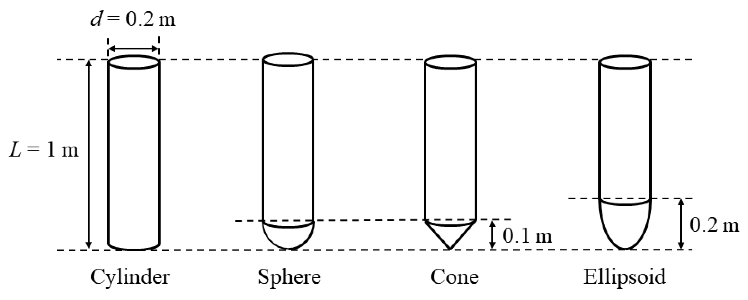
2. Problem Definition

In this study, a cylinder with a length of 1 m, a diameter of 0.2 m and a mass of 31.416 kg was first defined as the baseline model. It was considered a small-sized unmanned trans-media vehicle with a characteristic length of 1 m, as shown in Figure 1. The trans-media vehicle, developed by the first and second authors [26], can transform into a cylindrical body by the variant structure. Then, the water-entry processes were investigated by varying its mass, diameter-to-length ratio, water-entry angle and head shape.

In total, four arrays of computational models were designed for this study. The first array is shown in Figure 2. The cylinder with a length of 1 m and a diameter of 0.2 m was chosen, and its mass was either 15.708 kg, 31.416 kg or 47.124 kg. The second array (shown in Figure 3) consists of three cylinders with the same mass of 31.416 kg. In addition, Model 1 was 1 m in length and 0.2 m in diameter, Model 2 was 0.5 m in length and 0.2 m in diameter and Model 3 was 1 m in length and 0.4 m in diameter. The third array (shown in Figure 4) used the same cylinder with a length of 1 m, a diameter of 0.2 m and a mass of 31.416 kg, and the water-entry angle (α) was set to 30°, 45°, 60°, 75° or 90°. The fourth array is shown in Figure 5. The cylinders with a cylindrical head, a spherical head, a conical head or an ellipsoidal head were studied, and all of them were 1 m in length, 0.2 m in diameter and 31.416 kg in mass.

3. Numerical Methods

3.1. Governing Equations

The Ansys Fluent 19.4 software was employed to simulate the flow field of a falling object. The three-dimensional, incompressible and unsteady RANS equations were adopted as the governing equations [27], which include the continuity equation and the momentum conservation equations. The continuity equation for the fluid flow is expressed as follows:

$$\frac{\partial u}{\partial x}+\frac{\partial v}{\partial y}+\frac{\partial w}{\partial z}=0$$

(1)

where $u$, $v$ and $w$ represent the flow velocity in the $x$, $y$ and $z$ directions, respectively. The momentum conservation equations for the fluid flow are expressed as follows:

$$\frac{\partial u}{\partial t}+u\frac{\partial u}{\partial x}+v\frac{\partial u}{\partial y}+w\frac{\partial u}{\partial z}=f_x-\frac{1}{\rho }\frac{\partial P}{\partial x}+\frac{\mu +{\mu }_T}{\rho }\left(\frac{{\partial }^{2}u}{\partial x^2}+\frac{{\partial }^{2}u}{\partial y^2}+\frac{{\partial }^{2}u}{\partial z^2}\right)$$

(2)

$$\frac{\partial v}{\partial t}+u\frac{\partial v}{\partial x}+v\frac{\partial v}{\partial y}+w\frac{\partial v}{\partial z}=f_y-\frac{1}{\rho }\frac{\partial P}{\partial y}+\frac{\mu +{\mu }_T}{\rho }\left(\frac{{\partial }^{2}v}{\partial x^2}+\frac{{\partial }^{2}v}{\partial y^2}+\frac{{\partial }^{2}v}{\partial z^2}\right)$$

(3)

$$\frac{\partial w}{\partial t}+u\frac{\partial w}{\partial x}+v\frac{\partial w}{\partial y}+w\frac{\partial w}{\partial z}=f_z-\frac{1}{\rho }\frac{\partial P}{\partial z}+\frac{\mu +{\mu }_T}{\rho }\left(\frac{{\partial }^{2}w}{\partial x^2}+\frac{{\partial }^{2}w}{\partial y^2}+\frac{{\partial }^{2}w}{\partial z^2}\right)$$

(4)

where $P$ represents the fluid pressure; $f_x$, $f_y$ and $f_z$ represent the unit mass force in the $x$, $y$ and $z$ directions, respectively; $\rho$ represents the fluid density; $\mu$ represents the dynamic viscosity coefficient of fluid; and ${\mu }_T$ represents the turbulence eddy viscosity solved by the standard k–ε two-equation model [28].

3.2. VOF Method

The VOF method was employed in this study due to its high accuracy and good robustness in numerical simulations. For each grid cell in the flow field, the fluid volume fraction was defined as the ratio of the volume of the target fluid to the grid cell volume. Then, the free surface was tracked by calculating the value of the fluid volume fraction on each grid cell. The phase change of the flow field is presented by solving the governing equation for the fluid volume function [29], which is expressed as follows:

$$\frac{\partial F}{\partial t}+u\frac{\partial F}{\partial x}+v\frac{\partial F}{\partial y}+w\frac{\partial F}{\partial z}=0$$

(5)

where $F$ represents the fluid volume function.

3.3. 6DOF Motion Solver

The 6DOF motion solver can deal with the six-degrees-of-freedom motions of the falling rigid bodies in translational or rotational modes. The mass attributes, such as the mass, the center of gravity and the inertia tensor, were defined by the user-defined function. The displacement of the object was obtained by monitoring variations in the center of gravity. Assuming the variation of displacement is $\Delta s$ and the variation of time is $\Delta t$, the vertical force exerted by water on the object was obtained by solving the following formula:

$$v=\frac{\Delta s}{\Delta t}=\frac{s_{i+1}-s_i}{t_{i+1}-t_i}$$

(6)

$$a=\frac{\Delta v}{\Delta t}=\frac{v_{i+1}-v_i}{t_{i+1}-t_i}$$

(7)

$$F_{total}=Mg-F_w=Ma$$

(8)

where $v$ represents the vertical velocity, $a$ represents the vertical acceleration, $s$ represents the vertical displacement, $F_{total}$ represents the total vertical force, $M$ represents the mass and $F_w$ represents the vertical force exerted by water on the object.

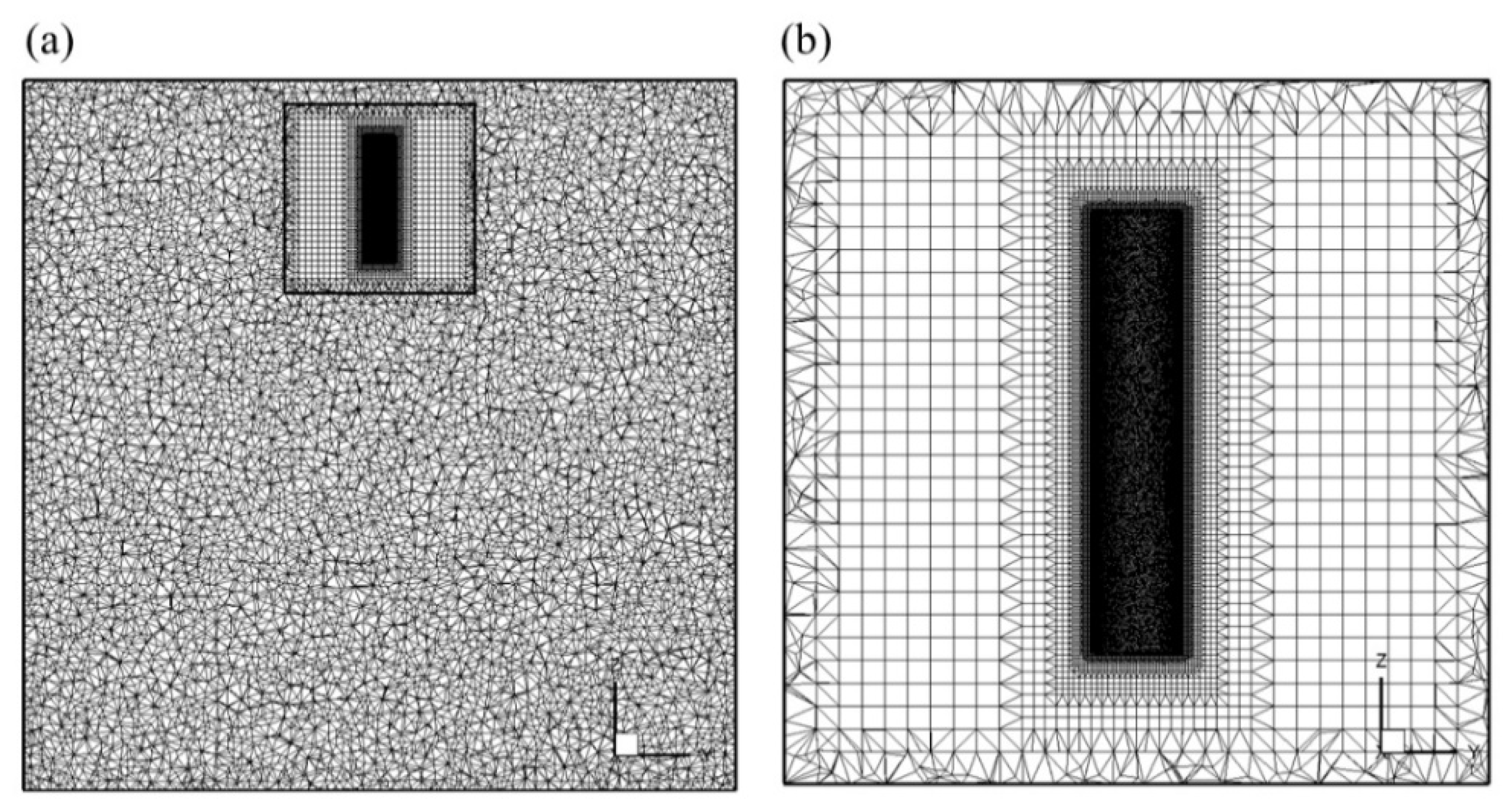
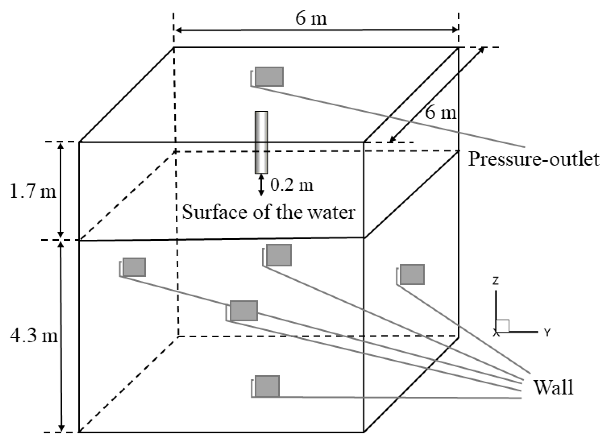
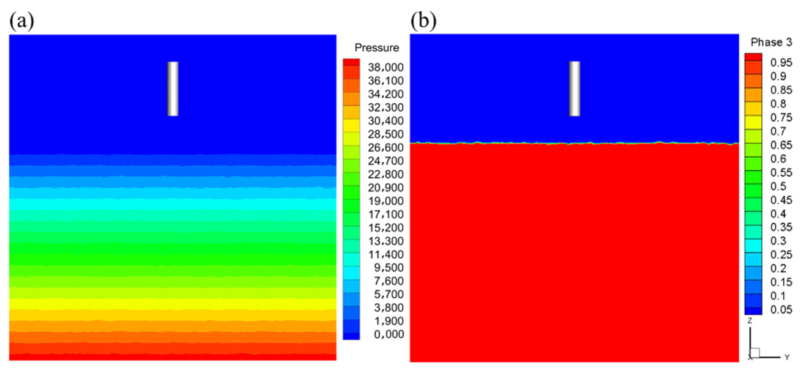
3.4. Grid, Boundary and Initial Conditions

The dynamic grid method, combining the spring-based smoothing algorithm and the mesh reconstruction algorithm, was adopted in the simulations. As shown in Figure 6a, the external flow field, denoted as the overall grid region, adopts the tetrahedral grid cells, due to the fact that the tetrahedral grid cells are more robust in the grid deformation compared with the hexahedral grid cells. As shown in Figure 6b, a square-shaped moving grid region is generated around the cylindrical body, which is dominated by the high-quality hexahedral grid cells for better spatial resolution. In order to accurately capture the water splashing phenomenon around the cylindrical body, the grid cells in the square-shaped moving grid region were specifically refined. In addition, the grid cells in the moving grid region were assumed to be rigid and to have moved together with the cylindrical body.

The computational region is a box of 6 m × 6 m × 6 m, as shown in Figure 7. The top surface is defined as the pressure-outlet boundary, and the remaining surfaces are defined as the solid wall boundaries. The initial location of the body’s bottom was set to 0.5 m above the water surface, and the initial velocity was assumed to be 5 m/s. Since the initial pressure field has a great impact on the water-entry process, it was necessary to perform a pretreatment in order to obtain a steady-state flow field as the initial flow field of an unsteady simulation. As shown in Figure 8a, the pressure field under the water was calculated using the following formula:

$$P=\rho gh$$

(9)

where $P$ represents the relative pressure, $\rho =998.2 \mathrm{kg}/{\mathrm{m}}^3$ represents the density of water, $g=9.81 \mathrm{m}/{\mathrm{s}}^2$ represents the acceleration of gravity, $h$ represents the depth of the water and the operating pressure is the standard atmospheric pressure of 101,325 Pa. The phase contour is shown in Figure 8b. Note that the volume fraction of air is 0, the volume fraction of water is 1 and the volume fraction in the air–water interface is between 0 and 1.

3.5. Grid Convergence Study

The baseline model defined in the previous section was used for the grid convergence study. Three grids with different densities were generated for the grid convergence study, as shown in

Table 2. The details of three grids for the grid convergency study.

Grid Name	Minimum Size of Moving Grid Region (mm)	Minimum Size of Overall Grid Region (mm)	$\mathbf{Number} \mathbf{of} \mathbf{Grid} \mathbf{Cells} (\times {10}^6)$
Grid 1	1.210	37.372	2.754
Grid 2	0.903	37.372	3.878
Grid 3	0.903	29.066	4.565

.

Figure 9 shows that the results for the three grids are very close to each other, indicating that the solution is sufficiently convergent. The following numerical simulations proceeded with the medium grid, denoted as Grid 2.

3.6. Validation of Numerical Methods

This section refers to the water-entry experiment involving a 3D wedge that was carried out by Yettou et al. [8]. The simulation results were compared with the experimental data in order to validate the accuracy of the numerical methods. As shown in Figure 10a, the simulated wedge had the same geometry as the experimental model. The initial velocity of the wedge was set to 0 m/s and the mass was set to 94 kg. The computational region was a box of 8 m × 8 m × 7.3 m, as shown in Figure 10b. The initial location of the wedge’s bottom was 1.3 m above the water surface and the water depth was 4 m.

As shown in Figure 11, the splash phenomenon was accurately captured. Figure 12 compares the numerical results and the experimental data. It can be seen that the numerical results agree well with the experimental data, indicating sufficient numerical accuracy for the current study.

4. Results and Discussion

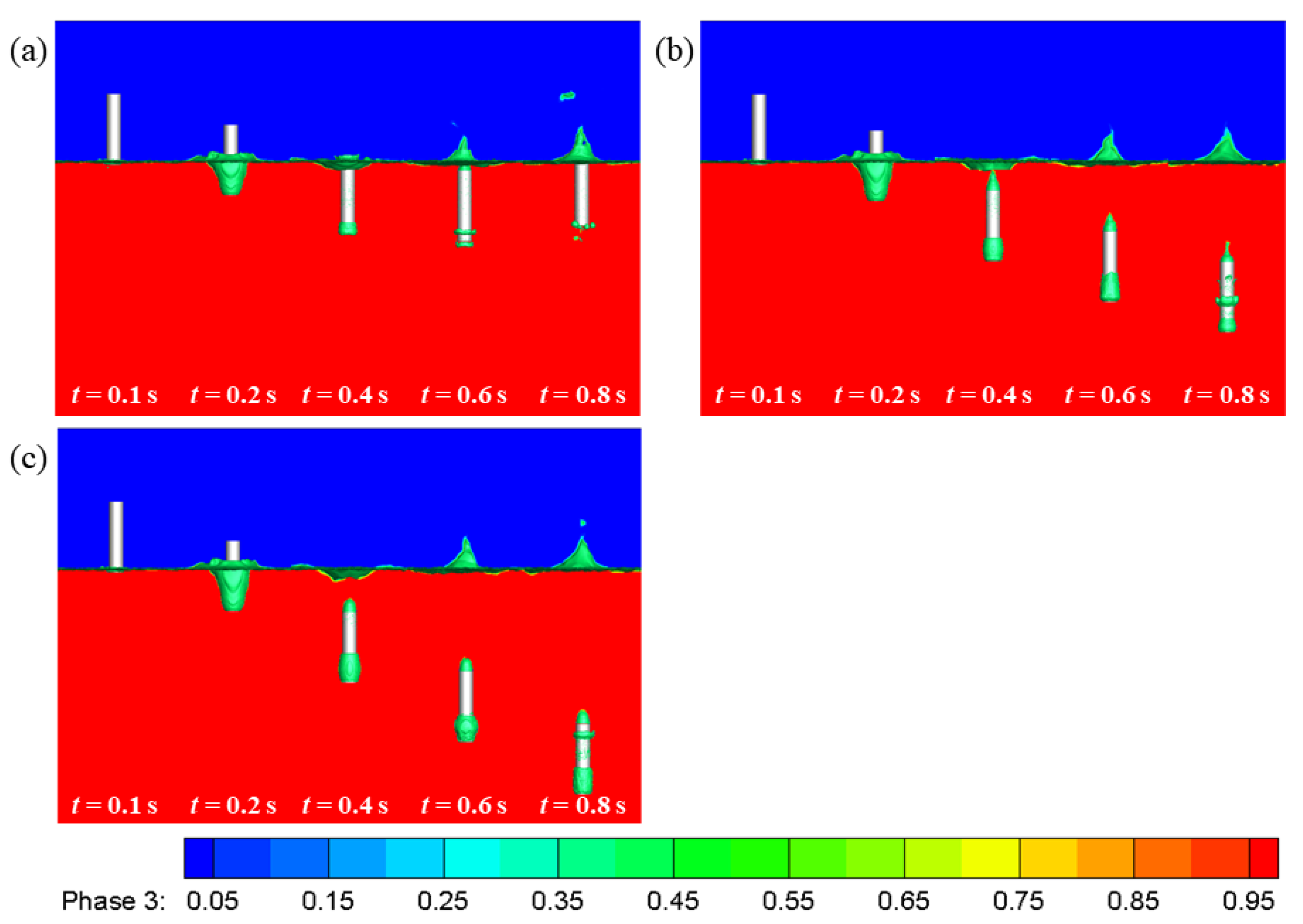
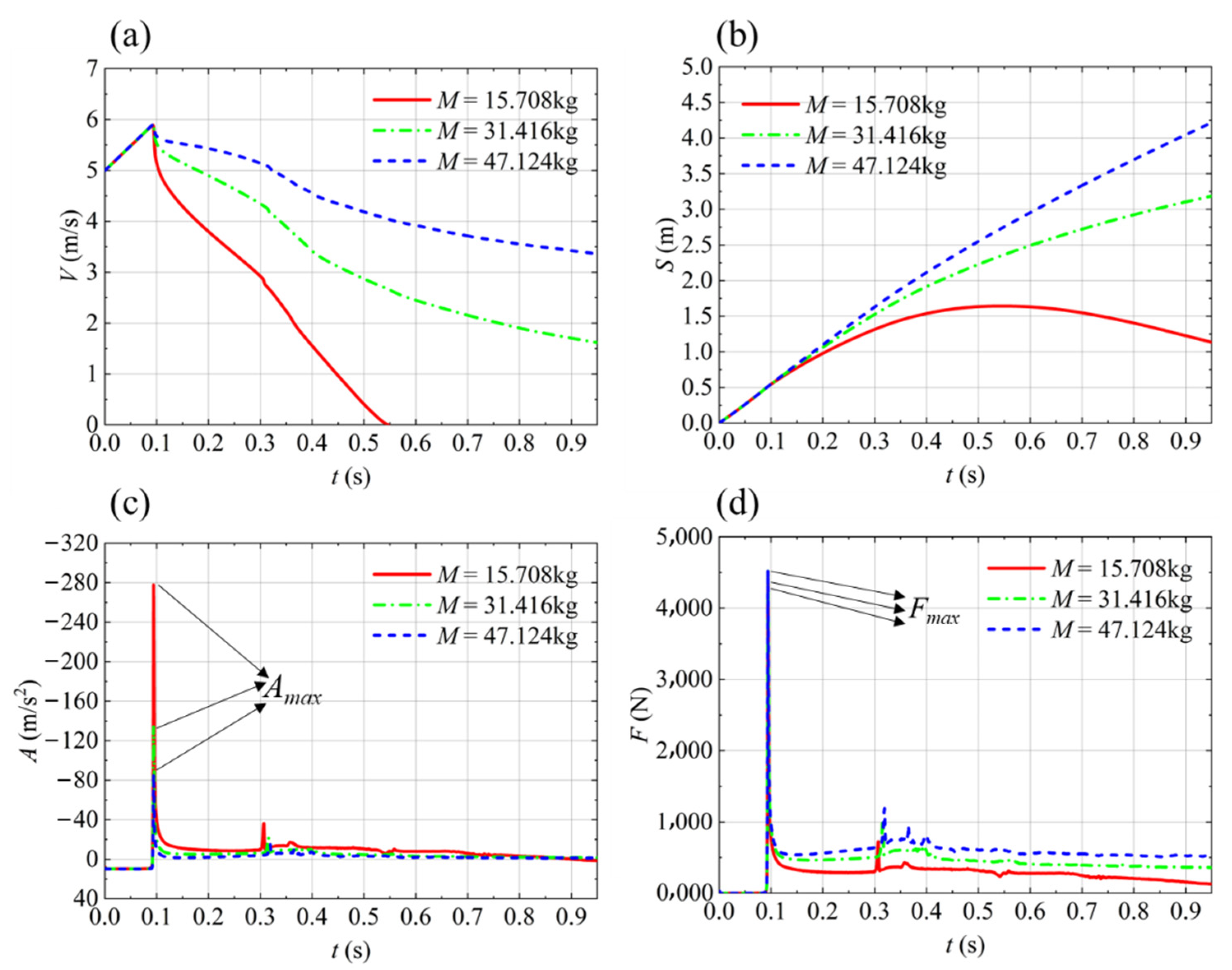
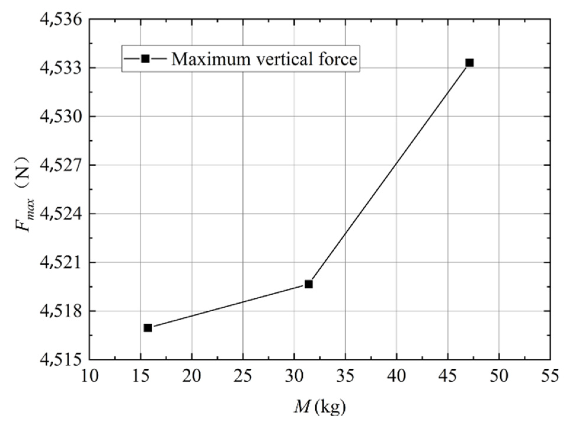
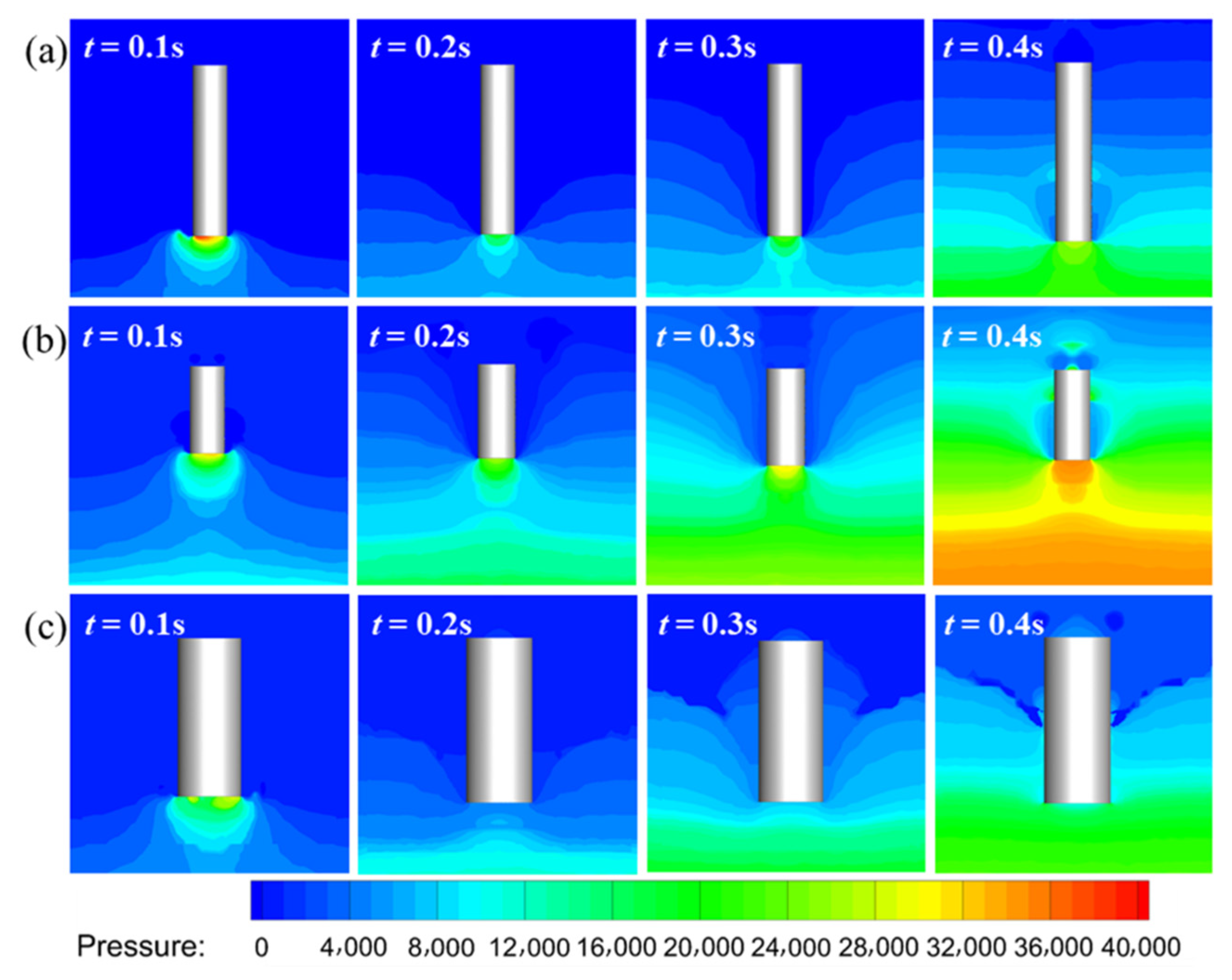
4.1. The Effect of Body Mass

This section studies the influence of body mass on the water-entry process. The geometries of the cylindrical bodies are shown in Figure 2. The inertia tensor of the cylinders is shown in

Table 3. The inertia tensor of the cylinders with varying masses.

Mass (kg)	Ixx (kg·m2)	Iyy (kg·m2)	Izz (kg·m2)	Ixy (kg·m2)	Ixz (kg·m2)	Iyz (kg·m2)
15.708	1.388	1.388	0.157	0.000	0.000	0.000
31.416	2.775	2.775	0.314	0.000	0.000	0.000
47.124	4.163	4.163	0.417	0.000	0.000	0.000

. In addition, the initial location of the body’s bottom was set to 0.5 m above the water surface and the initial velocity was assumed to be 5 m/s.

Figure 13 shows the instantaneous pressure contours of the cylinders with varying masses. When the cylinders touched the water surface, the pressure at their bottoms increased dramatically. After entering the water, the bottom pressure gradually decreased. In addition, the peak value of the bottom pressure was directly related to the body mass. As the mass increased, the bottom pressure also increased. Thus, it can be inferred that decreasing the mass can decrease the impact force. The instantaneous phase contours of the cylinders are shown in Figure 14. As expected, the cylinder with more mass fell faster under the water. Additionally, when the cylinders approached the water surface, they captured some air beneath them. In the figure, it is clear that some air was trapped beneath these cylinders, and the volume of the air trapped by the cylinder increased as the mass increased.

Figure 15 shows the time histories of the vertical velocity, the vertical displacement, the vertical acceleration and the vertical force. From the figure, it can be seen that before t = 0.094 s, the vertical acceleration of these cylinders was equal to the acceleration of gravity, and the vertical force exerted by the air was negligible. At t = 0.094 s, the cylinders began to touch the water surface and the vertical force exerted by water increased suddenly, confirming the observations in Figure 13. This peak impact load was the major reason for the damage that the vehicle structure sustained. A second peak impact load can be seen at the moment that the body completely fell into the water. However, compared with the first peak impact load, the second peak impact load was almost negligible. Further examination of the first peak load is presented in Figure 16. It was estimated that the peak load was approximately proportional to the square of the body mass. Thus, decreasing the mass of the body is an effective way to reduce the impact load. However, this may not be very practical due to the load-carrying requirements, so other methods of reducing the impact load have to be pursued as well.

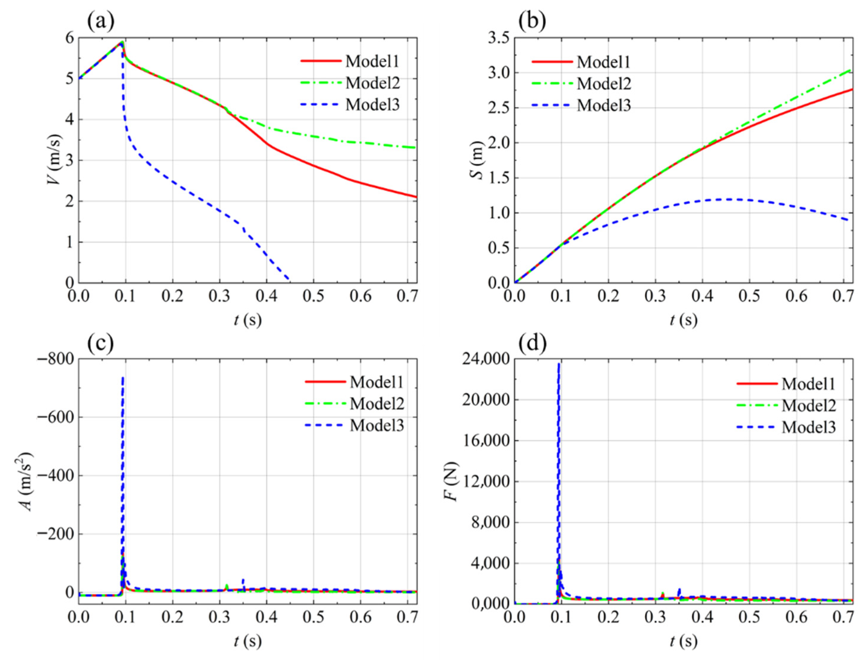
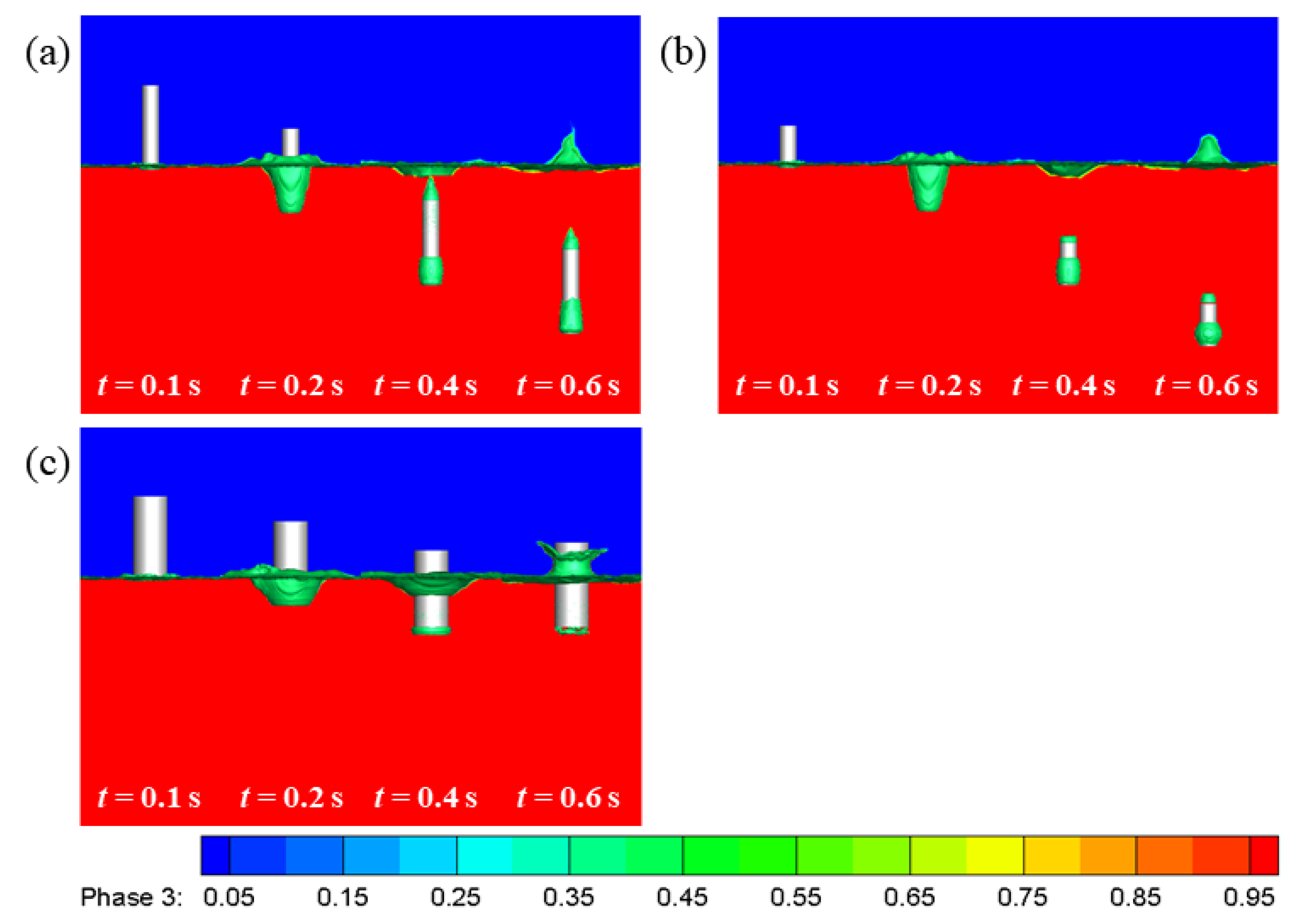
4.2. The Effect of Diameter-to-Length Ratio

In order to study the influence of the diameter-to-length ratio on the water-entry process, three cylinders with varying diameter-to-length ratios were chosen as the computational models, as shown in Figure 3. The inertia tensor of the cylinders is shown in

Table 4. The inertia tensor of the cylinders with varying diameter-to-length ratios.

Model	Ixx (kg·m2)	Iyy (kg·m2)	Izz (kg·m2)	Ixy (kg·m2)	Ixz (kg·m2)	Iyz (kg·m2)
Model 1	0.812	0.812	0.314	0.000	0.000	0.000
Model 2	2.775	2.775	0.314	0.000	0.000	0.000
Model 3	3.246	3.246	1.257	0.000	0.000	0.000

, and the initial conditions were the same as those in the previous section.

Figure 17 shows the instantaneous pressure contours of the cylinders. The cylinder with a lower diameter-to-length ratio (Model 1) produced a slightly higher peak pressure at the bottom. However, as shown in Figure 18, the cylinder with a diameter that was twice that of Model 1 (Model 3) experienced a peak impact load almost six times higher than that of Model 1 at the moment the body touched the water. The reason for this is that the volume is proportional to the cube of the diameter. Therefore, an increase in diameter greatly increased the total force, which is directly related to the volume of the displaced water. Due to the very high resistance, Model 3 was not fully immersed in water, as shown in Figure 19. On the other hand, decreasing the length has minor effects on the water-entry process. The behaviors of Model 1 and Model 2 were almost the same, except that noticeable differences were observed after the bodies completely entered the water. It can be concluded that the peak impact load is approximately proportional to the cube of the cylinder diameter, and decreasing the diameter of the cylinder is another effective way to reduce the peak impact load exerted by water on the object.

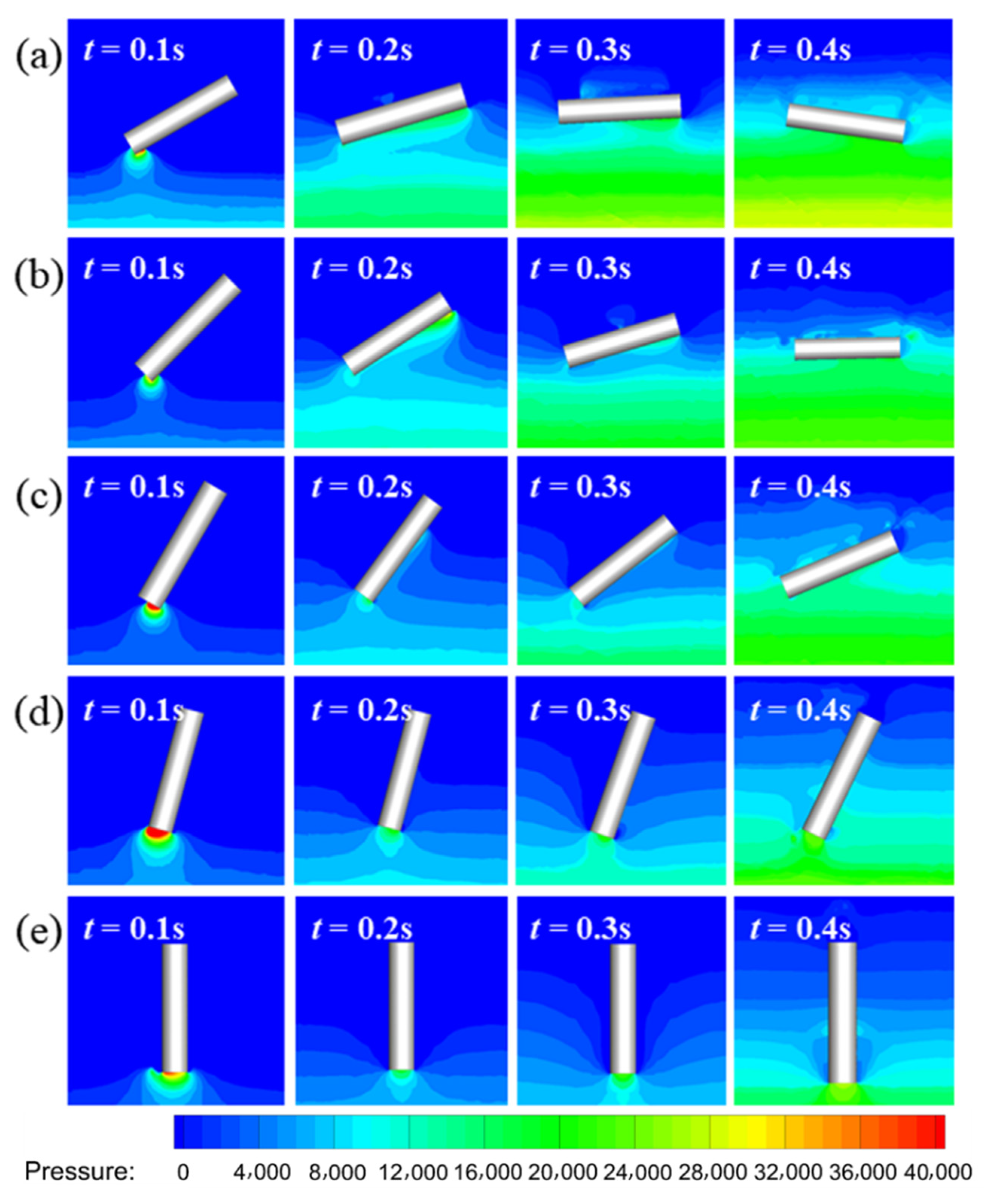
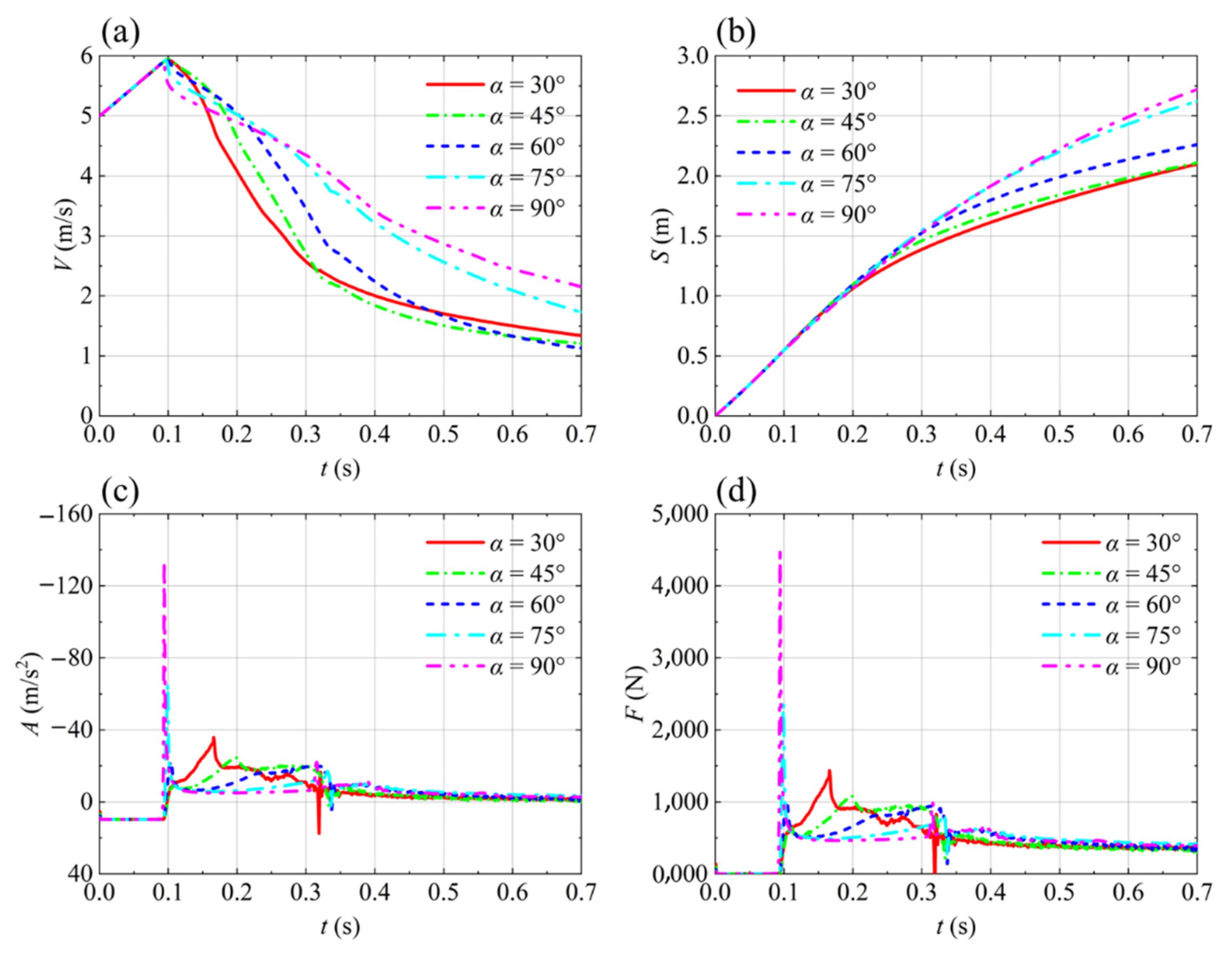
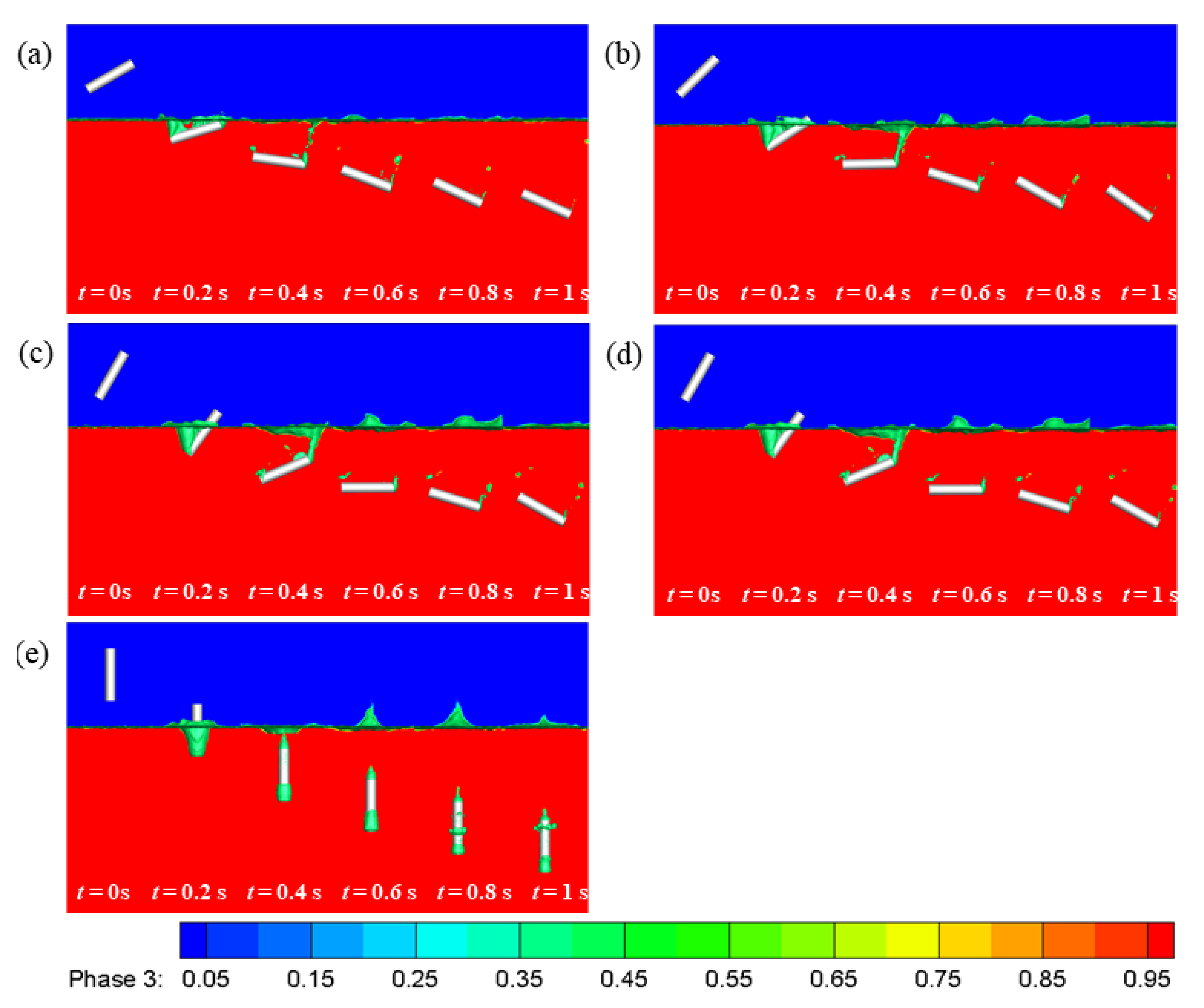
4.3. The Effect of Water-Entry Angle

In order to study the effect of the water-entry angle on the water-entry process, five water-entry angles (30°, 45°, 60°, 75° and 90°) were chosen, as shown in Figure 4. The inertia tensor of the cylinders is shown in

Table 5. The inertia tensor of the cylinders with varying water-entry angles.

Water-Entry Angle	Ixx (kg·m2)	Iyy (kg·m2)	Izz (kg·m2)	Ixy (kg·m2)	Ixz (kg·m2)	Iyz (kg·m2)
30°	2.775	0.929	2.160	0.000	0.000	−1.066
45°	2.775	1.545	1.545	0.000	0.000	−1.230
60°	2.775	2.160	0.929	0.000	0.000	−1.066
75°	2.775	2.610	0.479	0.000	0.000	−0.615
90°	2.775	2.775	0.314	0.000	0.000	0.000

, and the initial conditions were the same as those in the previous section.

Figure 20 shows the instantaneous pressure contours of the cylinders with varying water-entry angles. As expected, it can be seen that the peak pressure on the body decreased as the water-entry angle decreased. This is because a lower water-entry angle has increased the wettened area, and therefore has relieved the peak impact load. This observation was confirmed by further examination, as seen in Figure 21. It can be seen that the peak impact load at an angle of 90° was about 4.5 times larger than that at an angle of 60°. However, as shown in Figure 21d, the cylinder entering the water at a small water-entry angle experienced a bumpy force, which is unfavorable in some applications. Note that although a higher water-entry angle resulted in a higher peak load, the cylinder with a higher water-entry angle reached the target location at a faster speed, as shown in Figure 22. Depending on the requirements of the mission, an optimum water-entry angle should be pursued in practical applications.

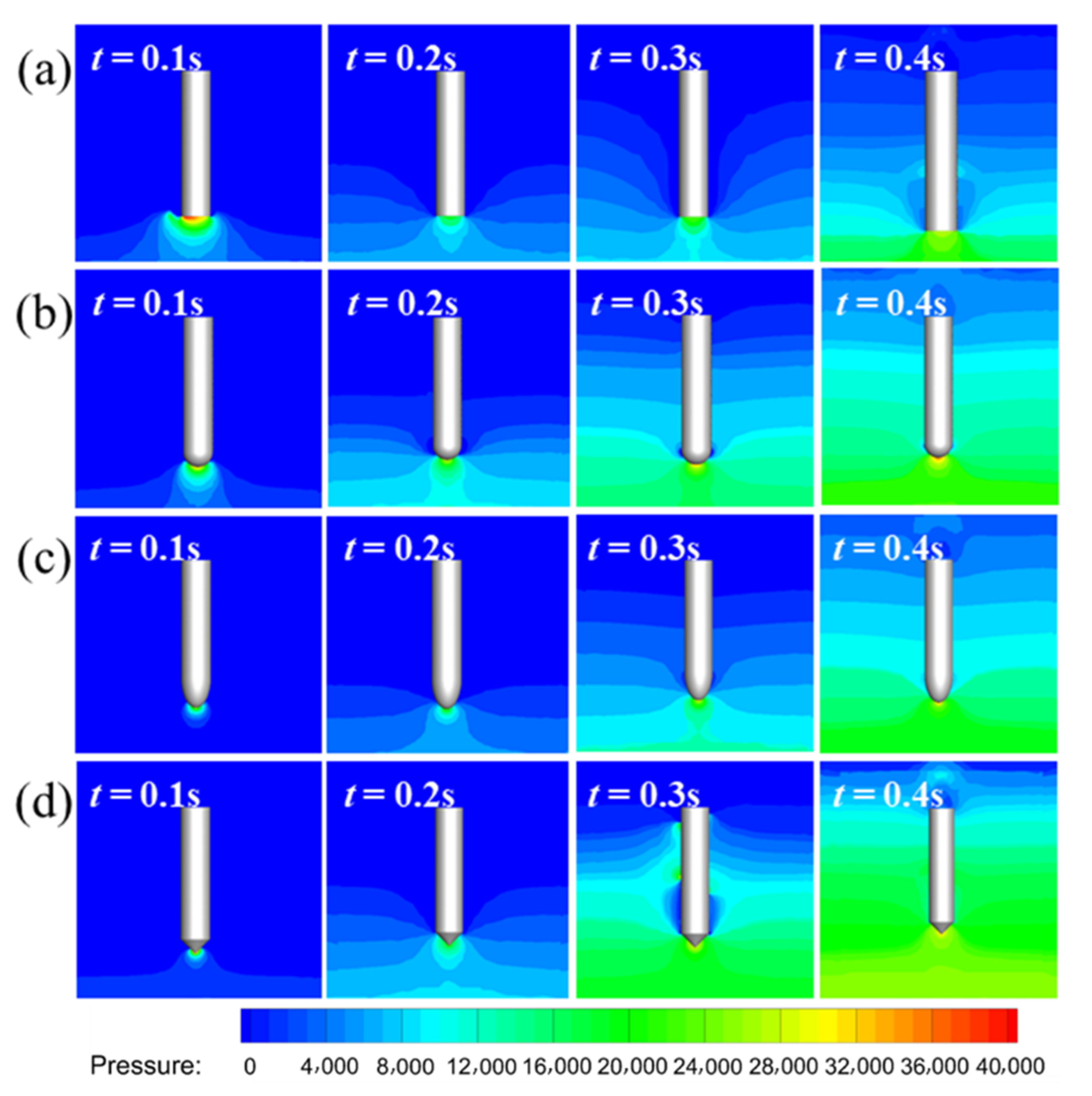
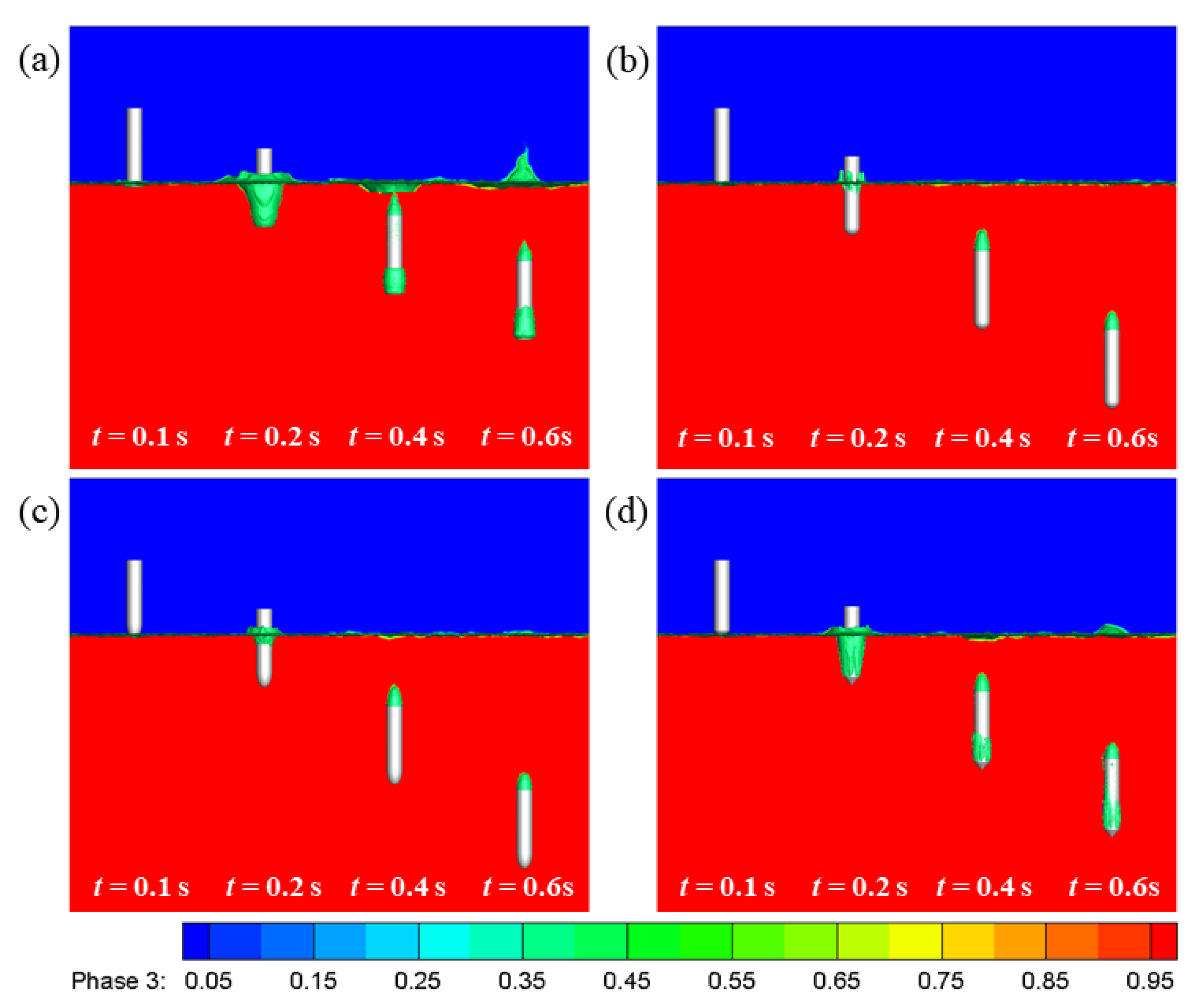
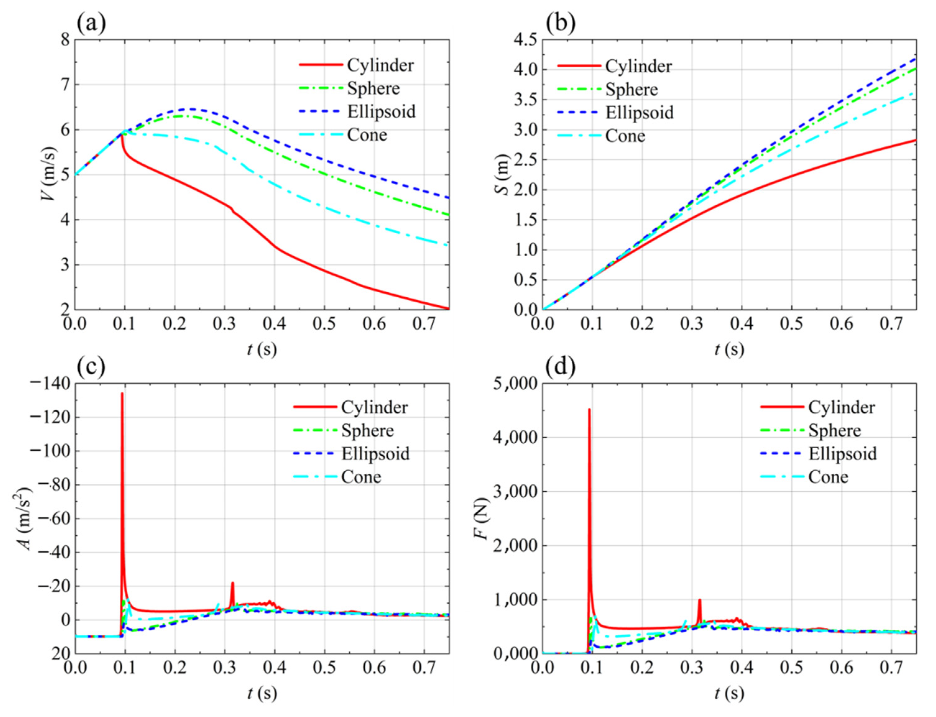
4.4. The Effect of Head Shape

In this section, the effect of head shape on the water-entry process is studied. The geometries of the chosen head shapes are shown in Figure 5. The inertia tensor of the cylindrical bodies is shown in

Table 6. The inertia tensor of the cylindrical bodies with varying head shapes.

Head Shape	Ixx (kg·m2)	Iyy (kg·m2)	Izz (kg·m2)	Ixy (kg·m2)	Ixz (kg·m2)	Iyz (kg·m2)
Cylinder	2.775	2.775	0.314	0.000	0.000	0.000
Sphere	2.278	2.278	0.314	0.000	0.000	0.000
Ellipsoid	1.833	1.833	0.314	0.000	0.000	0.000
Cone	2.278	2.278	0.314	0.000	0.000	0.000

, and the initial conditions were the same as those in the previous section.

The instantaneous pressure contours of the cylindrical bodies with varying head shapes are shown in Figure 23. It was observed that the cylindrical bodies with non-cylindrical head shapes had less pressure at the bottom compared to the cylinder. Figure 24 shows the instantaneous phase contours of the cylindrical bodies. Except for the cylinder and the cylindrical body with the cone head, the other models carried very few air bubbles at their heads. In addition, the cylinder with the ellipsoidal head had the fastest falling velocity among them.

Figure 25 shows the time histories of the cylindrical bodies. It can be seen that the vertical force decreased in the order of cylinder, cone, sphere and ellipsoid, and the vertical displacement increased in that order as well. Note that among the chosen head shapes, the peak vertical force of the cylinder with the ellipsoidal head was the lowest. Specifically, installing an ellipsoidal head can reduce about 94% of the peak impact load experienced by a cylindrical body. Similar observations were also made in the work of Shi et al. [23], who used a different numerical method, namely the ALE method. Compared with changing the water-entry angle, changing the head shape is a more effective means of reducing the peak impact load without any unfavorable effects.

5. Conclusions

The unsteady water-entry processes of small-sized cylindrical trans-media vehicles, with a characteristic length of 1 m, were investigated by solving the unsteady RANS equations using the VOF method, the dynamic grid method and the 6DOF motion solver. We found that the peak impact load, measured by the peak force exerted by water on the body, strongly depends on four key parameters, including the body mass, the diameter-to-length ratio, the water-entry angle and the head shape. In particular, the peak impact load was found to be approximately proportional to the square of the body mass or the cube of the cylinder diameter. Furthermore, installing an ellipsoidal head can reduce about 94% of the peak impact load experienced by a cylindrical body. Therefore, for practical application, decreasing the body mass, decreasing the diameter, entering the water at an optimum water-entry angle or installing an ellipsoidal head are recommended in order to relieve the peak impact load exerted by water on the body. Note that the current study mainly focuses on the water-entry processes of small-sized trans-media vehicles at a low speed (5 m/s). In some applications, bigger trans-media vehicles are designed to enter the water at a very high speed, thus the fluid compressibility, the cavitation effect and the Reynolds number effect cannot be neglected. In addition, fluid–solid interactions need to be addressed in future studies.

References

1. Von Kármán, T. The Impact on Seaplane Floats during Landing; NACA Technical Note No. 321; National Advisory Committee on Aeronautics: Washington, DC, USA, 1929. [Google Scholar]
2. Wagner, H. Über Stoß-und Gleitvorgänge an der Oberfläche von Flüssigkeiten. ZAMM-J. Appl. Math. Mech. Angew. Math. Mech. 1932, 12, 193–215. [Google Scholar] [CrossRef]
3. Zhao, R.; Faltinsen, O.; Aarsnes, J. Water Entry of Arbitrary Two-Dimensional Sections with and without Flow Separation. In Proceedings of the 21st Symposium on Naval Hydrodynamics, Trondheim, Norway, 24 June 1996; pp. 408–423. [Google Scholar]
4. Verhagen, J.H.G. The Impact of a Flat Plate on a Water Surface. J. Ship Res. 1967, 11, 211–223. [Google Scholar] [CrossRef]
5. Peseux, B.; Gornet, L.; Donguy, B. Hydrodynamic Impact: Numerical and Experimental Investigations. J. Fluids Struct. 2005, 21, 277–303. [Google Scholar] [CrossRef] [Green Version]
6. May, A.; Woodhull, J.C. The Virtual Mass of a Sphere Entering Water Vertically. J. Appl. Phys. 1950, 21, 1285–1289. [Google Scholar] [CrossRef]
7. Chu, P.C.; Gilles, A.; Fan, C. Experiment of Falling Cylinder through the Water Column. Exp. Therm. Fluid Sci. 2005, 29, 555–568. [Google Scholar] [CrossRef]
8. Yettou, E.-M.; Desrochers, A.; Champoux, Y. Experimental Study on the Water Impact of a Symmetrical Wedge. Fluid Dyn. Res. 2006, 38, 47. [Google Scholar] [CrossRef]
9. Alaoui, A.E.M.; Nême, A.; Tassin, A.; Jacques, N. Experimental Study of Coefficients during Vertical Water Entry of Axisymmetric Rigid Shapes at Constant Speeds. Appl. Ocean Res. 2012, 37, 183–197. [Google Scholar] [CrossRef]
10. Truscott, T.T.; Epps, B.P.; Belden, J. Water Entry of Projectiles. Ann. Rev. Fluid Mech. 2014, 46, 355–378. [Google Scholar] [CrossRef]
11. Van Nuffel, D.; Vepa, K.S.; De Baere, I.; Lava, P.; Kersemans, M.; Degrieck, J.; De Rouck, J.; Van Paepegem, W. A Comparison between the Experimental and Theoretical Impact Pressures Acting on a Horizontal Quasi-Rigid Cylinder during Vertical Water Entry. Ocean Eng. 2014, 77, 42–54. [Google Scholar] [CrossRef] [Green Version]
12. Takagi, K. Numerical Evaluation of Three-Dimensional Water Impact by the Displacement Potential Formulation. J. Eng. Math. 2004, 48, 339–352. [Google Scholar] [CrossRef]
13. Aquelet, N.; Souli, M.; Olovsson, L. Euler–Lagrange Coupling with Damping Effects: Application to Slamming Problems. Comput. Methods Appl. Mech. Eng. 2006, 195, 110–132. [Google Scholar] [CrossRef]
14. Stenius, I.; Rosén, A.; Kuttenkeuler, J. Explicit FE-Modelling of Fluid–Structure Interaction in Hull–Water Impacts. Int. Shipbuild. Prog. 2006, 53, 103–121. [Google Scholar]
15. Stenius, I.; Rosén, A.; Kuttenkeuler, J. Explicit FE-Modelling of Hydroelasticity in Panel-Water Impacts. Int. Shipbuild. Prog. 2007, 54, 111–127. [Google Scholar]
16. Wick, A.T.; Zink, G.A.; Ruszkowski, R.A.; Shih, T.I.P. Computational Simulation of an Unmanned Air Vehicle Impacting Water. In Proceedings of the 45th AIAA Aerospace Sciences Meeting, Reno, NV, USA, 8 January 2007. [Google Scholar]
17. Yang, Q.; Qiu, W. Numerical Simulation of Water Impact for 2D and 3D Bodies. Ocean Eng. 2012, 43, 82–89. [Google Scholar] [CrossRef]
18. Abraham, J.; Gorman, J.; Reseghetti, F.; Sparrow, E.; Stark, J.; Shepard, T. Modeling and Numerical Simulation of the Forces Acting on a Sphere during Early-Water Entry. Ocean Eng. 2014, 76, 1–9. [Google Scholar] [CrossRef]
19. Qu, Q.; Hu, M.; Guo, H.; Liu, P.; Agarwal, R.K. Study of Ditching Characteristics of Transport Aircraft by Global Moving Mesh Method. J. Aircr. 2015, 52, 1550–1558. [Google Scholar] [CrossRef]
20. Facci, A.L.; Porfiri, M.; Ubertini, S. Three-Dimensional Water Entry of a Solid Body: A Computational Study. J. Fluids Struct. 2016, 66, 36–53. [Google Scholar] [CrossRef] [Green Version]
21. Xiao, T.; Qin, N.; Lu, Z.; Sun, X.; Tong, M.; Wang, Z. Development of a Smoothed Particle Hydrodynamics Method and Its Application to Aircraft Ditching Simulations. Aerosp. Sci. Technol. 2017, 66, 28–43. [Google Scholar] [CrossRef] [Green Version]
22. Xiang, G.; Wang, S.; Soares, C.G. Study on the Motion of a Freely Falling Horizontal Cylinder into Water Using OpenFOAM. Ocean Eng. 2020, 196, 106811. [Google Scholar] [CrossRef]
23. Shi, Y.; Pan, G.; Yan, G.-X.; Yim, S.C.; Jiang, J. Numerical Study on the Cavity Characteristics and Impact Loads of AUV Water Entry. Appl. Ocean Res. 2019, 89, 44–58. [Google Scholar] [CrossRef]
24. Wang, X.; Shi, Y.; Pan, G.; Chen, X.; Zhao, H. Numerical Research on the High-Speed Water Entry Trajectories of AUVs with Asymmetric Nose Shapes. Ocean Eng. 2021, 234, 109274. [Google Scholar] [CrossRef]
25. Wu, X.; Chang, X.; Liu, S.; Yu, P.; Zhou, L.; Tian, W. Numerical Study on the Water Entry Impact Forces of an Air-Launched Underwater Glider under Wave Conditions. Shock Vib. 2022, 2022, 4330043. [Google Scholar] [CrossRef]
26. Deng, F.; Sun, X. Trans-Media Unmanned Aerial Vehicle Device And Control Method Thereof. PCT/CN2021/098354, 4 June 2021. Chinese Patent Application No. 202110441374.7, 23 April 2021. [Google Scholar]
27. Anderson, J.D. Governing Equations of Fluid Dynamics. In Computational fluid dynamics; Springer: Berlin, Germany, 2009; pp. 15–51. [Google Scholar]
28. Launder, B.E.; Spalding, D.B. Lectures in Mathematical Models of Turbulence; Academic Press: New York, NY, USA, 1972. [Google Scholar]
29. Hirt, C.W.; Nichols, B.D. Volume of Fluid (VOF) Method for the Dynamics of Free Boundaries. J. Comput. Phys. 1981, 39, 201–225. [Google Scholar] [CrossRef]
Figure 1. A concept of the next-generation unmanned trans-media vehicle developed by the first and second authors [26].
Aerospace 09 00805 g001
Figure 2. The cylindrical bodies with varying masses.
Aerospace 09 00805 g002
Figure 3. The cylindrical bodies with varying diameter-to-length ratios.
Aerospace 09 00805 g003
Figure 4. The cylindrical bodies with varying water-entry angles.
Aerospace 09 00805 g004
Figure 5. The cylindrical bodies with varying head shapes.
Aerospace 09 00805 g005
Figure 6. Grid topology. (a) Overall grid region; (b) Moving grid region.
Aerospace 09 00805 g006
Figure 7. Boundary conditions.
Aerospace 09 00805 g007
Figure 8. Initial conditions. (a) Pressure contour; (b) Phase contour.
Aerospace 09 00805 g008
Figure 9. Grid convergence study. (a) Time history of vertical velocity; (b) Time history of vertical acceleration; (c) Time history of vertical displacement; (d) Time history of vertical force.
Aerospace 09 00805 g009
Figure 10. The setup of the validation case. (a) Geometry of the 3D wedge; (b) Computational region.
Aerospace 09 00805 g010
Figure 11. Instantaneous phase contours of the 3D wedge. Blue color represents air and red color represents water.
Aerospace 09 00805 g011
Figure 12. Comparisons between the numerical results and the experimental data. (a) Time history of vertical velocity; (b) Time history of vertical displacement.
Aerospace 09 00805 g012
Figure 13. Instantaneous pressure contours of the cylinders with varying masses. (a) M = 15.708 kg; (b) M = 31.416 kg; (c) M = 47.124 kg.
Aerospace 09 00805 g013
Figure 14. Instantaneous phase contours of the cylinders with varying masses. (a) M = 15.708 kg; (b) M = 31.416 kg; (c) M = 47.124 kg.
Aerospace 09 00805 g014
Figure 15. Comparisons between the time histories of the cylinders with varying masses. (a) Vertical velocity; (b) Vertical displacement; (c) Vertical acceleration; (d) Vertical force.
Aerospace 09 00805 g015
Figure 16. Comparisons between the first peak impact loads of the cylinders with varying masses.
Aerospace 09 00805 g016
Figure 17. Instantaneous pressure contours of the cylinders with varying diameter-to-length ratios. (a) Model 1; (b) Model 2; (c) Model 3.
Aerospace 09 00805 g017
Figure 18. Comparisons between the time histories of the cylinders with varying diameter-to-length ratios. (a) Vertical velocity; (b) Vertical displacement; (c) Vertical acceleration; (d) Vertical force.
Aerospace 09 00805 g018
Figure 19. Instantaneous phase contours of the cylinders with varying diameter-to-length ratios. (a) Model 1; (b) Model 2; (c) Model 3.
Aerospace 09 00805 g019
Figure 20. Instantaneous pressure contours of the cylinders with varying water-entry angles. (a) α = 30°; (b) α = 45°; (c) α = 60°; (d) α = 75°; (e) α = 90°.
Aerospace 09 00805 g020
Figure 21. Comparisons between the time histories of the cylinders with varying water-entry angles. (a) Vertical velocity; (b) Vertical displacement; (c) Vertical acceleration; (d) Vertical force.
Aerospace 09 00805 g021
Figure 22. Instantaneous phase contours of the cylinders with varying water-entry angles. (a) α = 30°; (b) α = 45°; (c) α = 60°; (d) α = 75°; (e) α = 90°.
Aerospace 09 00805 g022
Figure 23. Instantaneous pressure contours of the cylindrical bodies with varying head shapes. (a) Cylinder; (b) Sphere; (c) Ellipsoid; (d) Cone.
Aerospace 09 00805 g023
Figure 24. Instantaneous phase contours of the cylindrical bodies with varying head shapes. (a) Cylinder; (b) Sphere; (c) Ellipsoid; (d) Cone.
Aerospace 09 00805 g024
Figure 25. Comparisons between the time histories of the cylindrical bodies with varying head shapes. (a) Vertical velocity; (b) Vertical displacement; (c) Vertical acceleration; (d) Vertical force.
Aerospace 09 00805 g025