1. Introduction
High-fidelity finite element (FE) models of aero-engines contain a great number of degrees of freedom (DOFs), generally millions [
1]. These models can provide precise predictions of many vibration problems, including blade-casing rubbing [
1,
2] and rotor–stator coupled vibration [
3]. However, the high number of DOFs greatly increases the computational cost, especially when conducting geometry optimization or transient analysis.
Reducing the number of DOFs is imperative to accelerate computation. Directly reducing the mesh density is unreasonable due to the complex geometries of the substructures, such as the blade. An intuitive approach is applying substructural model synthesis techniques, such as the Craig–Bampton method [
4,
5], to the substructures, including the stators. This method is widely applied. It can reduce the number of DOFs by retaining fewer modes, but the geometric details become implied in the reduced matrix of the substructure. Cyclic symmetry analyses can significantly reduce the simulation time. The cyclically periodicity is the necessary condition for cyclic symmetry analyses, however this is often broken in multiple-stage rotors and stators.
Alternatively, finding physical replacements for the substructures with similar vibration characteristics and a small number of DOFs can accelerate the computation with acceptable accuracy on the complete aero-engine level. In high-fidelity FE models, the rotors and stators are circumferential quasi-periodic structures, containing a large portion of the DOFs. The former involves many severe vibration problems, which need an exact mesh. Conversely, the vibration of the latter is moderate, due to their high rigidity. Therefore, identifying physical replacements for the stators can improve the design process without affecting the main dynamics of the engine.
The homogenization method aims at substituting heterogeneous periodic or quasi-periodic structures with dynamically equivalent homogeneous structures [
6]. Its applications are wide-ranging, including two main areas. The first is at the material level, involving polycrystals [
7] and particle-reinforced composites [
8], etc. The second is at the structural level, dealing with metamaterials [
9,
10], whose unit cells have a micro-scale length compared to the length of the assembled structure. The unit cell is the smallest repeatable substructure. When the unit cell has a medium-scale length, which is the case for stators, homogenization is possible based on the long-wave assumption [
11,
12]. This assumption states that a structure can be considered homogenous if the wavelength is much larger than the length of the unit cell. Relevant research has been conducted on trusses [
13,
14] and framed structures [
15,
16], among other things, which encouraged us to design a physical replacement based on the long-wave characteristics.
An intuitive approach is to use topological methods [
17,
18] to optimize the geometry and the material distribution of the physical replacement. However, the range of the optimized parameters is huge, thus the process is time-consuming. The optimal geometry can be complex, which can even increase the number of DOFs. Therefore, introducing parameter constraints is critical to determine the search direction and accelerate the search process.
The analytical description of long-wave motion is needed to bridge the gap between the pristine stators and their physical replacements. In this way, we divide the homogenization approach into two steps. The first step is producing a continuous analytical description of the pristine structure. Many approaches have been developed for such a task, such as the representative volume element [
19] (RVE) method and asymptotic homogenization [
20] (AH). These two methods involve obtaining the equivalent elastic modulus of the unit cell. However, the vibration motions of stators are complex, including flexural–torsional coupled vibration. To describe these motions analytically, the macroscopic mechanical properties are needed to be identified in advance. Nevertheless, these kinds of analytical descriptions cannot be directly applied in engineering models. To overcome this issue, the second step which is to substantiate the analytical description into a physical replacement is indispensable. Finally, the physical replacement can be assembled in the whole structure.
In this paper, we design physical replacements of the stators in an aero-engine based on homogenization, aiming at reducing the number of DOFs. Owing to the wave vibration consistency [
21], the structural vibration is viewed from the wave motion perspective. The principle is to make the physical replacements have the same long wave characteristics as pristine stators. To do that, two homogenizations are conducted subsequently. The first involves the analytical description of the flexural and flexural–torsional coupled wave motions. The second comprised substantiating the analytical descriptions into physical replacements with three selected cross-sections.
Specifically, we first use the wave finite element method [
22,
23,
24] (WFEM) to investigate the wave characteristics of the stators (
Section 3). Based on the dispersion curves and wave shapes, the wave motions are divided into flexural and flexural–torsional coupled motion, respectively. Second, we derive the analytical descriptions of these two wave motions and extract twelve mechanical properties from the stator cells (
Section 4). Next, we substantiate the two analytical descriptions into physical replacements with I, box, and open cross-sections (
Section 5). Then, we implement the genetic algorithm (GA) to initiate the search process, which is very efficient thanks to the analytical expressions (
Section 4 and
Section 5). Finally, we validate the quality of the physical replacements by comparing the modal frequencies with the pristine stators through commercial software (
Section 5).
2. Problem Formulation
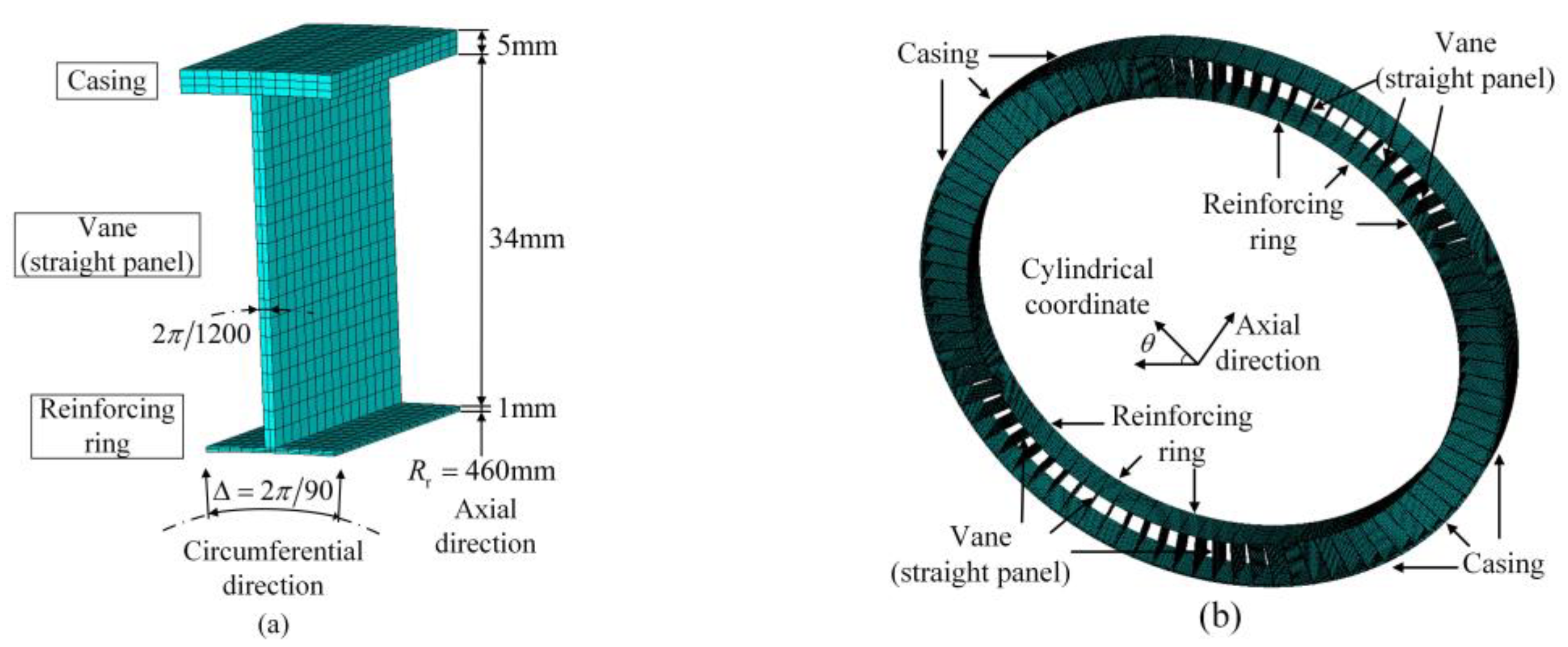
The finite element (FE) model of a single-stage stator is illustrated in
Figure 1. This model contains three components: casing, vane, and reinforcing ring. For simplicity and without loss of generality, the vanes are simplified to the straight panels. The element is SOLID185 in ANSYS and the material parameters are elastic modulus
, Poisson’s ratio
and density
. The angle of one cell is 4° and thus a full circle contains 90 cells. The stator with straight panels possesses much fewer DOFs compared with the one with real vanes. But the total number of the DOFs in
Figure 1 still reaches 626,400.
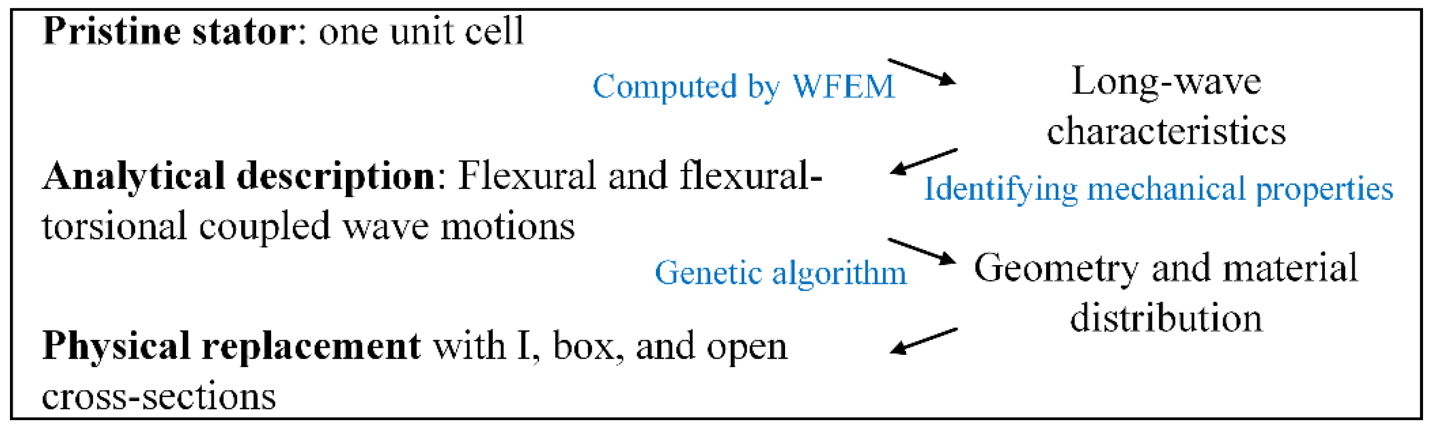
We first investigate the wave characteristics of the stator along the circumferential direction by WFEM. From the knowledge of the dispersion curves and the wave shapes, we find that the flexural and flexural-torsional coupled wave motions are dominant in long-wave cases. Two homogenizations are successively initiated. The details of the technical route are shown in
Figure 2.
The first homogenization involves identifying analytical descriptions for two wave motions. Two analytical beams, the flexural Timoshenko (FT) and flexural-torsional coupled Timoshenko (FTCT) beams, are introduced to describe the two wave motions, respectively. Twelve mechanical properties associated with these two beams are estimated preliminarily according to the static analyses. Based on the initial estimation, we then employ GA to further optimize the properties.
The second homogenization refers to substantiating the two analytical descriptions into physical replacements with I, box, and open cross-sections. We derive analytical expressions of the mechanical properties based on geometric and material parameters of the cross-sections. Then we use GA to search for these parameters. Finally, for verification, we conduct modal analyses on the pristine stator and the physical replacements by the commercial packages, and compare the differences in natural frequencies.
4. Analytical Description
The first homogenization involves identifying analytical descriptions of the stator. According to the wave motions computed in
Section 3, we select the flexural Timoshenko (FT) and flexural-torsional coupled Timoshenko (FTCT) beams. In this section, we first preliminarily estimate the macroscopic mechanical properties. Based on the estimation, we subsequently use the genetic algorithm to optimize the properties.
4.1. Timoshenko Beams
A segment of the beam with an arbitrary cross-section is shown in
Figure 6. The centroid and the shear center of this cross-section are
and
, respectively, between which
is the distance. The flexural displacement in
direction, the bending slope and the torsional rotation with respect to
direction are donated by
,
, and
, respectively.
The motion equations of the FT beam [
34] is
where
and
are the bending and shear rigidities, respectively;
is the mass per unit length;
is the mass moment of inertia with respect to the shear center per unit length.
The motion equations of the FTCT beam [
35,
36] can be expressed as
where
is the mass moment of inertia with respect to the centroid per unit length;
and
indicate the torsional and warping rigidities.
To obtain the wave characteristics of the FTCT beam, let
where
is the wavenumber along
direction;
,
, and
are the magnitudes of these displacements. Introducing Equation (10) into Equation (9) yields
Assuming Equation (11) has nontrivial solutions, namely
, one can obtain
The details of
are shown in
Appendix A. Solving Equation (12) yields the dispersion curves of the FTCT beam. In such a way, the dispersion curves of the FT beam can also be obtained, which is omitted for brevity.
4.2. Identifying Mechanical Properties
Equations (8) and (9) possess a total of 12 mechanical properties. Four properties including
,
,
, and
determine the FT beam, and eight properties including
,
,
,
,
,
,
, and
determine the FTCT beam. The mechanical definitions and analytical formulas are listed in
Table 2. We can divide the properties into two categories. The first category contains the four rigidities, whose identification is based on the four static analyses of the unit cell. The second category contains
,
,
, and
, which can be computed by the analytical integrals. It is to be noted that the FT and FTCT beams share the same properties
and
, but the properties
and
are different.
Let us demonstrate how to use the four static analyses to estimate the four rigidities.
Figure 7 illustrates the details of these analyses implemented on the unit cell. We can observe that the left boundary is fixed and the external loads are all applied on the right boundary. Please note that we use the average displacement in a cross-section as the equivalent displacement. Lagrange interpolation is then employed to construct the fitting function of these displacements.
The first static analysis identifies the neutral axis and the torsional center of the unit cell. As shown in
Figure 7, we apply a bending moment
with respect to the initial node whose radius is 460 mm. The radius of the node who has the minimum stress is used as the updated radius
of the neutral axis. Please note that the relationship between the polar wavenumber
and the wavenumber
is
A torsional moment is subsequently applied to the cell. The torsional center is set to the node with minimum displacement.
The second static analysis identifies the bending rigidity
. We apply a bending moment
with respect to the neutral axis. As aforementioned, the discrete equivalent displacements are fitted to the deformed function
, whose average curvature is
as shown in
Table 2. Therefore,
can be obtained by the first formula in
Table 2.
The third static analysis identifies the shear rigidity
. We apply a shear force
on the right boundary. In the same way, we can obtain the deformed function
. Extracting the average rotation
with respect to the neutral axis from the deformed cell, we can obtain the shear rigidity by the second formula in
Table 2.
The fourth static analysis identifies the torsional rigidity
and the warping rigidity
. We apply two torsional moments
and
with respect to the torsional center. The average rotation angle of every cross-section is used to construct the fitting function
. We can obtain two linear equations by the third formula in
Table 2, which can yield
and
together.
Let us demonstrate how to obtain the left four properties. We use each element of the unit cell as the unit mass
and the unit volume
, as listed in the fourth and fifth formulas in
Table 2, respectively, where
is the distance from the
to the shear center;
is the distance from
to the centroid;
is the total mass of the unit cell. The two integrals are substituted with the discrete summations. Then solving the last four formulas successively yields the four properties.
It is to be noted that the properties
and
are different for FT and FTCT beams. An intuitive explanation is that the flexural directions of these two motions are in different directions according to the wave shapes in
Figure 5. Specifically, the flexural motion of the FT beam is in the radial direction, while the torsional motion tends to couple with the flexural motion who has a weak rigidity in its vibration direction. As shown in
Figure 7, we use the flexural direction ⅰ and ⅱ for FT and FTCT beams, respectively.
4.3. Optimizing Properties
In this section, we optimize the eight properties for the analytical description based on the initial properties identified from the last section and the genetic algorithm. The identified rigidities and the left four properties are listed in
Table 3 (initial rigidities) and
Table 4, respectively.
On this basis, employing the genetic algorithm to further improve the accuracy of the rigidities becomes convenient and very fast, generally in seconds, due to the analytical formulas. One can use commercial software packages such as function ga() in Matlab to initiate the search process.
We use the initial rigidities as a reference, and set the search range around these rigidities. Specifically, the upper and lower bounds are the initial rigidities multiplied by two coefficients, such as (0.5, 2). The objective function is set to
where
is the polar wave-number at the
natural frequency of the analytical description;
is the polar wave-number of the pristine stator, namely 1,2,3… Then, the genetic algorithm can be initiated and the optimal rigidities are listed in
Table 3. Please note that for the FT beam, the optimized rigidities are
and
.
4.4. Dispersion Curves
The dispersion curves of the analytical descriptions are illustrated in
Figure 8. The red lines denote the curves of the initial beams; the blue lines denote the curves of the optimized beams; the black lines denote the curves of the pristine stator. We can observe that the dispersion curves of the four analytical beams have good agreement with those of the pristine stator in long-wave cases. Furthermore, the optimized beams show a better performance. It indicates that GA improves the accuracy of these rigidities based on the initial estimation.
For the flexural wave motion (wave 1), the separation of the curves is at polar wavenumber 15, corresponding to six cells () in one wavelength. It reaches the edge of the long-wave assumption.
For the flexural-torsional coupled wave motion (waves 3 and 4), the curves meet from the polar wavenumber 5. This may be an intrinsic error because the dispersion curve of the analytical description is bound to start at polar wavenumber 0 at 0 Hz. But the dispersion curve of wave 3 starts at polar wave-number 1.25 at 0 Hz. It means that the analytical FTCT beam cannot exactly describe the wave motion in this frequency band. But when we substantiate the FTCT beam into a physical replacement, the error is mitigated as illustrated in the next section.
5. Physical Replacements
The second homogenization substantiates the analytical descriptions into physical replacements. To do that, we select I, box, and open cross-sections, and derive analytical formulas for the mechanical properties based on the geometric and material parameters. Then we employ GA to search for optimal cross-sections. The modal analyses are finally performed on a physical replacement to estimate the differences in natural frequencies and modal shapes.
5.1. Mechanical Properties of Selected Cross-Section
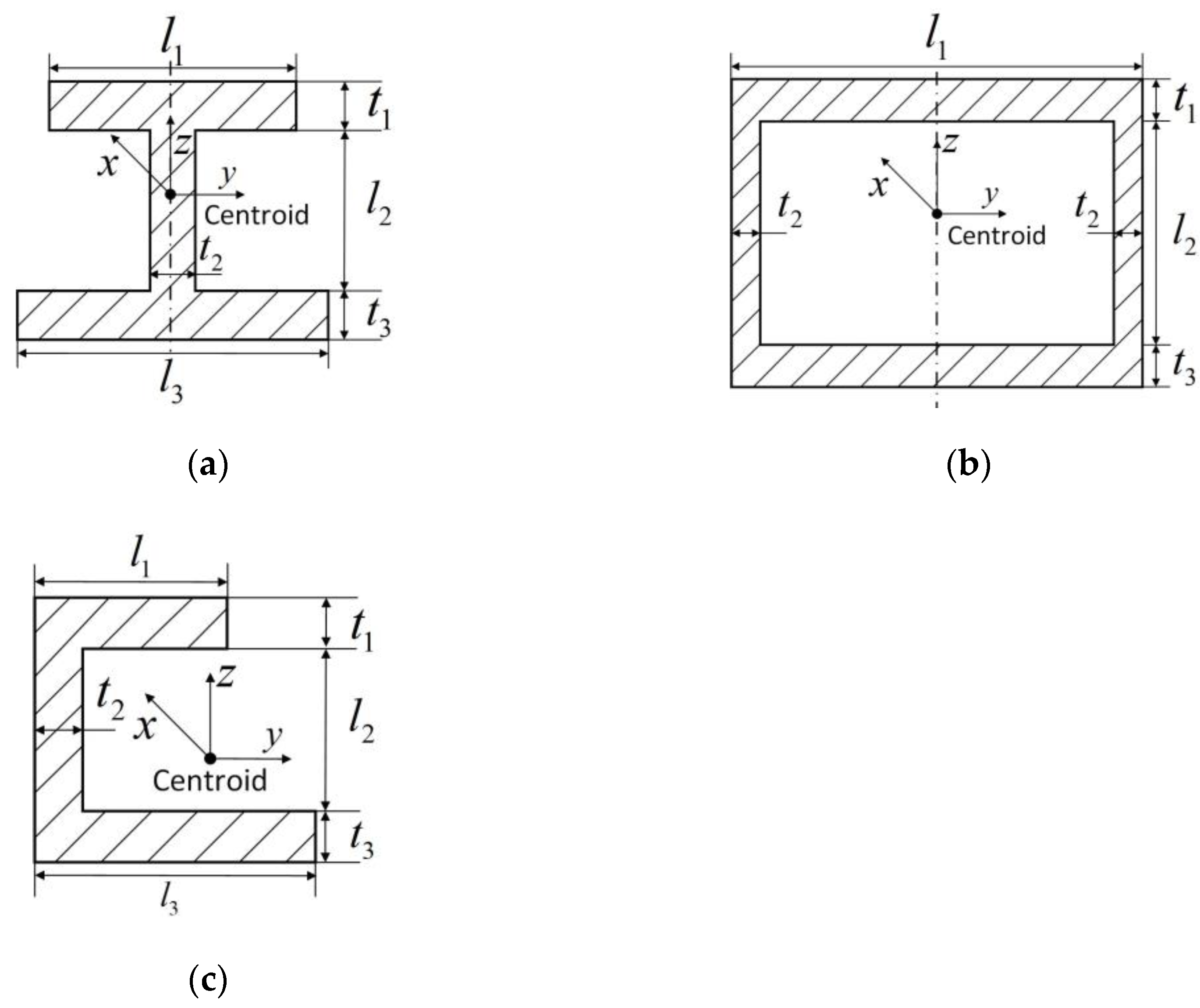
The I, box, and open cross-sections are shown in
Figure 9a–c, respectively. The former two are set to be bilaterally symmetric following the geometric features of the stator. The geometric parameters are thicknesses
,
,
and lengths
,
,
. The coordinates origin locates at the centroid. The formulas of the mechanical properties are listed in
Table 5. It is to be noted that the difference between
Table 2 and
Table 5 is that all the integrals in
Table 5 can be computed analytically owning to the uniform cross-sections.
The first step is identifying the centroid. The distance from the centroid to the bottom is
where
is the static moment of the cross-section with respect to the bottom;
is the distance from the surface element
to the bottom;
is the area of the cross-section. For the I and box cross-sections, the centroid locates on its symmetric axis. But for the open cross-section, we also need the distance from the centroid to the left edge. It can be obtained by replacing
with
, which is the distance from
to the left edge.
The second step is identifying the torsional center. Let us demonstrate the sectorial coordinate system [
38]. An example is the open cross-section as shown in
Figure 10. A sectorial axis initiates from
to
and
and terminates at
. The sectorial coordinate [
39] is defined as
where
is the vertical distance from the micro unit
to the centroid as shown in
Figure 10. In analogy with the product of inertial in Cartesian coordinates, the sectorial products of inertia are
where
is the thickness of the micro unit
as shown in
Figure 9c. The torsional center locates at
where
and
are inertia moments with respect to the
and
axes, respectively.
For the I and box cross-sections, the torsional center locates on each symmetric axes due to the bilateral symmetry. The I cross-section contains two sectorial axes, which lie on the center lines of the upper and lower plates, respectively. The sectorial axis of the box cross-section is a loop line.
The third step performs the analytical formulas in
Table 5 to obtain the four properties of the FT beam and the eight properties of the FTCT beam. But the warping rigidity needs further demonstration.
To calculate
, we suggest using the principal sectorial coordinate
. That is to let
where
indicates the sectorial coordinate with respect to the torsional center. The warping moment of inertia can be expressed as
In this section, we use six geometric parameters of the selected cross-sections together with three material parameters , and to explicitly express the eight properties. Hence, we can directly relate the nine parameters to the wave characteristics.
5.2. Searching for Parameters of Cross-Sections
We use GA to search for the parameters of the cross-sections. The objective function is expressed as
where
is the optimal properties of the analytical beams in
Table 3 and
Table 4. Please note that the FT and FTCT beams possess four and eight properties, respectively. The optimization constraints are listed in
Table 6.
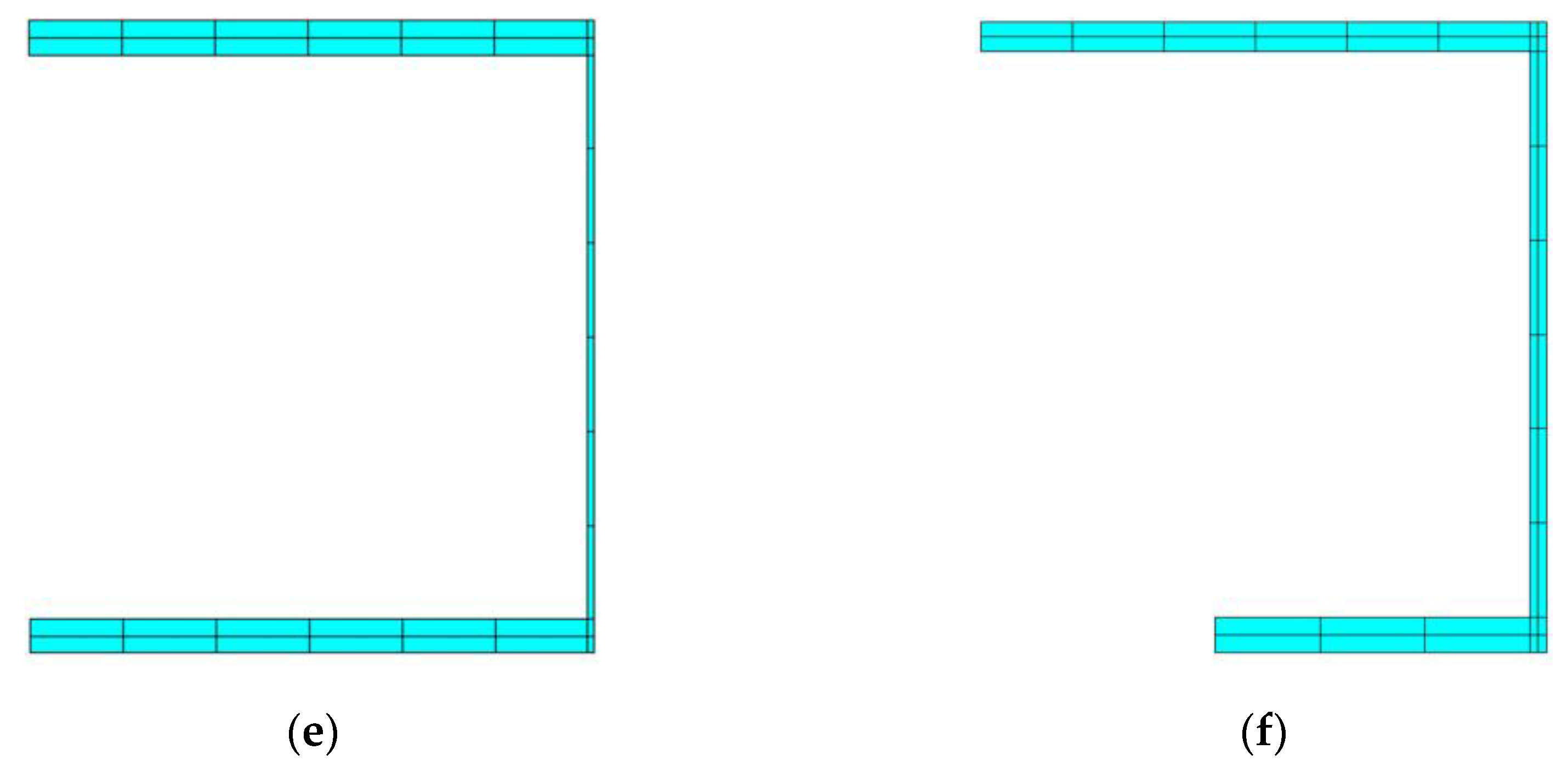
The genetic algorithm finds six cross-sections. The I, box, and open cross-sections of the FT beams are shown in
Figure 11a,c,e, respectively. The cross-sections of the FTCT beams are shown in
Figure 11b,d,f, respectively. We can observe that the centroid and the torsional center in
Figure 11a,c are overlapped and locate at each geometric center. It denotes that the flexural-torsional coupled motion will not occur. For the left four cross-sections, the centroid and the shear center are in different positions, and thus the coupled wave motion will occur.
5.3. Dispersion Curves
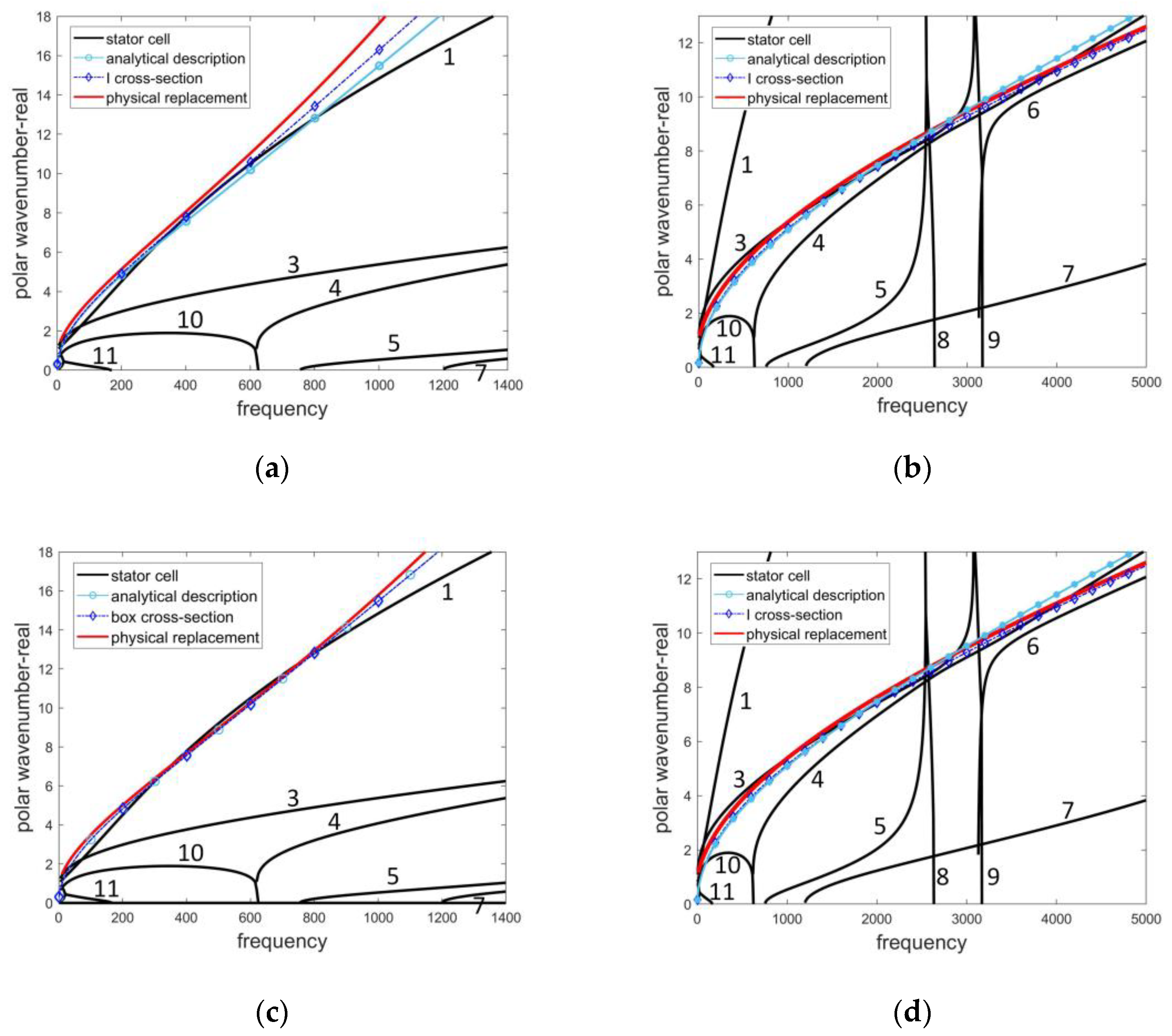
Once dragging the cross-sections in
Figure 11 along the circumferential direction, we can construct the unit cells of the physical replacements in FE packages. WFEM is subsequently used to obtain the dispersion curves.
Figure 12 illustrates the dispersion curves of the six cases, which are of the FT and FTCT beams with the I (
Figure 12a,b), box (
Figure 12c,d), and open (
Figure 12e,f) cross-sections, successively.
The black lines are the numerical dispersion curves of the pristine stator. The solid lines with circles are the analytical dispersion curves of the analytical descriptions which are the same as those of the optimal beams in
Figure 8. The dash-dot lines with rhombus are the analytical dispersion curves of the six cross-sections found by GA in the last section. The red lines are the numerical dispersion curves of the physical replacements with I, box, and open cross-sections.
The dispersion curves of the I and box cross-sections consist with the curves of each physical replacement. The valid range of the polar wavenumber is from 0 to 10 or 13. It verifies the accuracy of the formulas in
Table 5.
The dispersion curves of the I, box, and open cross-sections also have good agreement with the curves of the analytical descriptions, especially in
Figure 12c,d,f. It indicates that GA shows a good performance in searching the desired cross-sections. The best homogenization is using the physical replacement with the box cross-section to describe the flexural motion of the stator cell in
Figure 12c.
Concerning the difference observed in
Figure 8, it is mitigated after substantiating the FTCT beam into the I and box cross-sections as shown in
Figure 12b,d.
However, errors occur between the dispersion curves of the open cross-section and its physical replacement. This may be caused by the higher evaluation of flexural rigidity. We assume that the flexural direction is in the
axis as shown in
Figure 9c, which can be different with the real flexural motion of the open section. Because the flexural motion tends to occur in the direction with lower flexural rigidity. This leads to the high dispersion curves of the physical replacements compared to those of the analytical beams as illustrated in
Figure 12e,f. The open cross-section is not recommended due to its complex geometry.
5.4. Verification: Modal Analysis
This verification selects the case of using box cross-section to describe the flexural motion of the pristine stator. It is the case shown in
Figure 12c. A full-circle FE model of the physical replacement with the box cross-section is established by the FE packages, as shown in
Figure 13. The modal analysis is subsequently conducted, and the natural frequencies of the flexural motion along the radial direction are listed in
Table 7.
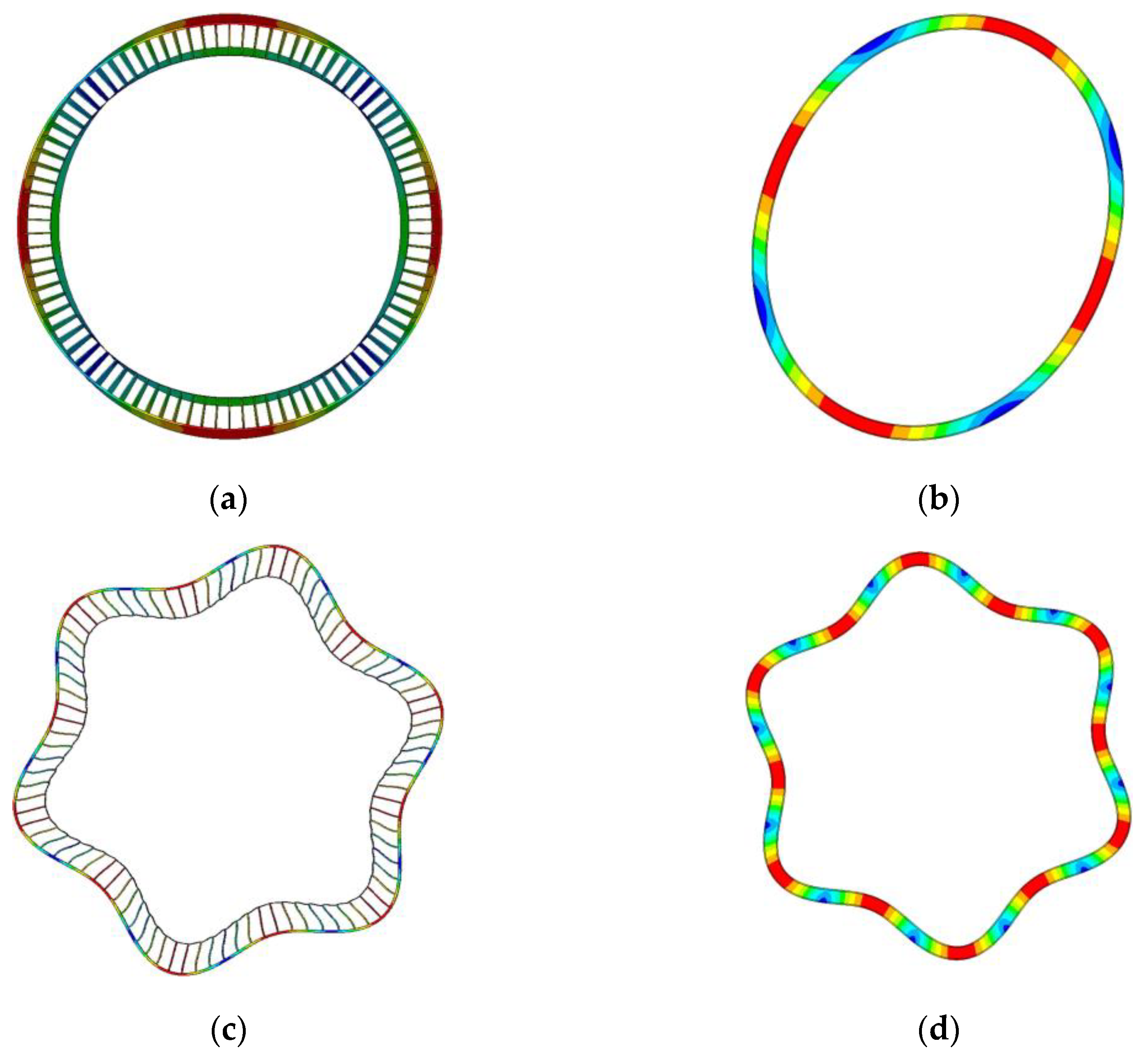
We can observe that the relative errors from the nodal diameters 2 to 5 are much higher than those of the nodal diameters 6–15. This is because the mode shapes of the nodal diameters 2–5 associated with the stator do not only vibrate in the radial direction, but the axial direction also. Examples including the 2nd and 6th nodal diameter modes are illustrated in
Figure 14. With the number of the nodal diameter increasing, the mode shape evolves into the pure flexural motion, and the relative error decreases. When it reaches 17, there are only five cells (
) in a wavelength, resulting in an increment of the relative error. It means that with the polar wavenumber increases, fewer cells exist in a wavelength to describe the wave motion and thus the relative error increases. It enters the edge of the long-wave assumption in the stator case.
It can be concluded that the physical replacement with the box cross-section is able to describe the flexural motion of the pristine stator. This model can be implemented in the aero-engine FE model, and meanwhile, it decreases the DOFs from 626,400 to 60,480.
Besides, the decrease of the DOFs generally denotes that the physical replacement can save computational costs. But it can be different depending on the application and the selected algorithm. To acquire the data in
Table 7, we use the Block Lanczos algorithm to compute the 100 modal frequencies of the pristine stator and the physical replacement with box cross-section, respectively. The calculation times of the former is 249.734 s and that of the latter is 50.796 s. Therefore, the calculation time is reduced by around 80%.
6. Conclusions
In this paper, a two-step homogenization modeling approach for the stator of an aero-engine is proposed based on the long-wave assumption. The corresponding physical replacement, containing fewer DOFs, keeps the same vibration features as the pristine stator in terms of the wave motion.
Calculating the wave characteristics of the stator is the premise of homogenization modeling. Through the wave finite element analysis, we find that there are 7 propagating waves in the long-wave cases, which can be divided into the flexural and flexural-torsional coupled wave motions.
Through the first homogenization, the analytical description between the pristine stator and the physical displacement is derived, avoiding the time-consuming direct search process of the physical replacements. We introduce the flexural Timoshenko (FT) and flexural-torsional coupled (FTCT) beams to describe the two wave motions. Twelve macroscopic mechanical properties in the analytical descriptions are identified from the stator cell based on the static analyses and the genetic algorithm. Results show that the dispersion curves of the analytical beams consist with those of the pristine stator in long-wave cases.
Through the second homogenization, the physical replacements with I, box, and open cross-sections are obtained. We derive the formulas to express the twelve mechanical properties by the geometric and material parameters of the cross-sections. The genetic algorithm is employed to initiate the optimization, and six optimal cross-sections are found. The search process is very fast owning to the analytical expressions. Results show that the dispersion curves of the I and box cross-sections consist with those of the pristine stator. But for the open cross-section, errors occur due to the rigidity overestimation, which is not recommended.
By using the proposed homogenization method, a full-circle physical replacement with the box cross-section is established for a single-stage stator FE model in engineering. The effectiveness of the physical replacement is verified through modal analyses. Comparing with the pristine stator, the relative error of the natural frequencies of flexural motions with nodal diameters 6–15 is less than 5%. The physical replacement decreases the DOFs from 626,400 to 60,480, and the calculation time is reduced by around 80%.


