Quantitative Measurement Method for Ice Roughness on an Aircraft Surface

Abstract

When an aircraft passes through clouds containing supercooled water droplets, the leading edge’s surface will gradually accumulate ice. Ice surface roughness is an important parameter affecting the local convective heat transfer coefficient and the water collection coefficient, which in turn affect the ice’s shape. However, because the surface roughness of aircraft icing is a transient value varying in time and space, it is extremely difficult to measure with existing methods in real time. In this study, a noncontact ultrasonic pulse-echo (UPE) technique is applied to characterize the ice roughness of an airfoil model’s surface. A multilayer model with equivalent bead-like roughness profiles is established to study the effects of changes in ice roughness on ultrasonic echo signals. A series of simulations indicated that ice roughness can be measured quantitatively and effectively in the range of [11.6, 120] μm. Based on these simulations, an experimental UPE device was developed to measure echo signals on top of the ice corresponding to surface roughness. The results show that for both the regular and irregular surface roughness samples, the maximum relative error in the roughness is less than 15%. Meanwhile, we designed and supplemented the experiment with the NACA-0012 airfoil model to realize the online measurement of ice roughness in an icing research tunnel.

1. Introduction

When an aircraft is cruising or approaching landing under a state of icing, the shape of the ice, with its rough surface, can alter the characteristics of the leading edge, thus threatening flight safety [1]. The formation of surface roughness varies irregularly in space and time [2], and it is related to heat transfer, fluid flow, and droplet properties [3]. A large number of research results show that both small- and large-scale roughness (i.e., ice shape) can significantly alter the unsteady flow separation pattern and the formation of a dynamic-stall vortex, leading to increased drag, reduced stall at a given angle of attack, and reduced maximum lift [4,5]. In a typical aircraft’s icing process, micrometer-scale roughness forms when droplets impact the surface and freeze in the shape of spherical caps in a randomly distributed fashion in the initial stages [6]. Especially for glaze ice, with this increase in surface roughness, convective heat transfer and water collection efficiency are enhanced in local areas, leading to higher rates of growth in the ice’s thickness, thereby affecting the final shape of the ice [3,7,8].

The accurate measurement and modeling of the initial ice’s roughness in real time are known to significantly improve the accuracy of ice shape prediction [9]. In glaze icing, the bead-like ice roughness model has been proposed to improve the accuracy of calculations [2,6,7]. This fully analytical model is based on experimental measurements, but these are limited to a roughness height of hundreds of micrometers [10]. During the initial stage of icing, the roughness maximum height (RMH) near the stagnation point is very small, with an average of between a few micrometers and hundreds of micrometers [11].

To date, many techniques have been developed to measure ice roughness and thickness, and these can mainly be divided into contact and noncontact methods. Traditional contact measurement techniques are inefficient and subject to large human error. Typical examples of such methods are ice tracing and hot wax molding [12,13], both of which damage the ice structure during the measurement process, resulting in a loss of roughness detail. To address the need for undamaged roughness measurements, a variety of noncontact techniques have been investigated using close-up photogrammetric approaches [10,14,15] or laser-based scanning [3,16,17,18] to reconstruct the ice contours. With close-up photography [10] and videography [14,15], it is possible to reconstruct the three-dimensional contours of ice shapes using multiple cameras. However, owing to the limitations imposed by the available camera arrangement angles and glaze ice’s optical characteristics, such techniques are subject to large measurement errors and require complex data processing. At present, laser-based 3-D scanning techniques are widely and successfully used to measure ice roughness. These techniques have high precision and can obtain both small- and large-scale roughness at the same time [16]. Unfortunately, 3-D-scanning techniques need a developer to be sprayed on the surface because of the transparent nature of ice, making it impossible to measure roughness in real time. Similarly, in the digital image projection (DIP) technique, grids of a certain size are projected onto the surface of the measured object, and 3-D structures are measured by examining the degree of grid distortion [19]. This technique also requires that the measured object be opaque. In summary, current ice measurement techniques are limited in their capabilities regarding the dynamic acquisition of small-scale roughness in the initial icing stage, and, in particular, they lack the ability to measure the real-time evolution of icing. There is no effective technique available to measure the distribution and evolution of small-scale roughness during the early stage of icing, with one reason for this being the continuous spatiotemporal changes in roughness that occur throughout the icing accretion process. Therefore, there is an urgent need to develop a technique that can measure the surface roughness of aircraft icing in real time.

Ultrasonic pulse-echo (UPE) techniques, as a form of waveguide-based, real-time measurement technique, have been employed to determine the thickness of accreted ice on aircraft, as well as its material properties. Pulse-echo waves are used as an information carrier to measure an object’s attributes or thickness through the parameters’ change of echo signal [20]. For instance, Hansman and Kirby [21] were the first to use piezoelectric transducers to measure the ice accretion of aircraft, and the feasibility of their technique was verified in corresponding flight experiments. Hansman et al. [22] also found that the characteristic parameters of an ultrasonic signal were affected by the surface characteristics of ice. More recently, Liu et al. [23] reported that both glaze ice and rime ice could be characterized by frequency-dependent ultrasonic pulse attenuation. Compared with measurements of ice thickness and density, the measurement of ice surface roughness is more difficult because of its spatiotemporal variations [11].

In developing UPE techniques for the study of ice roughness, reference can be made to their application in other fields. In a typical biomedical application, Hériveaux et al. [24] established a sinusoidal equivalent model to characterize the evolution of bone–implant interface roughness using quantitative ultrasound. Their results showed that both soft tissue thickness and interface roughness caused the attenuation of the ultrasonic reflection coefficient. In a materials science study, Ma et al. [25] developed a novel ultrasonic reflection coefficient phase spectrum technique to characterize the interfacial roughness of coatings and were thus able to measure roughness values from 6.2 to 12.7 μm. They also analyzed the effect of coating porosity on the roughness measurements. Okajima et al. [26] reported a method to estimate the Manning roughness coefficients for a planar region directly from the peak-to-peak value of a reflected ultrasonic pulse wave. All these studies suggest that the roughness of an element’s structure will reduce the ultrasonic interface reflection coefficient to an extent that should enable the application of a UPE technique to measure ice surface roughness.

Although UPE techniques have been used to measure interfacial and surface roughness in previous studies, the scenarios in which they have been applied are very different to those encountered in aircraft icing. At present, there is no effective acoustic model describing the effect of ice surface roughness on an ultrasonic signal. However, it should be possible to develop such a model on the basis of the high-precision icing calculation method [7,26,27] in which the ice roughness elements on the ice’s surface are considered to be like beads, with the roughness being controlled mainly by the height and contact angle. This bead-like model is mainly derived from experimental results [28] and has been applied to the experimental study [29] of water film’s flow characteristics on rough surfaces. Then, to measure ice roughness in real time, the quantitative relationships between the roughness and the characteristic parameters of echo signals need to be studied.

In this paper, a novel UPE technique combined with an equivalent roughness model is developed for quantitatively characterizing small-scale roughness in the initial stage of aircraft icing. First, it is assumed that the surface roughness profile of aircraft icing during the initial stage is similar to that of a collection of beads. The changes in surface roughness are controlled by adjusting the bead height and contact angle. Bead height is confirmed to be the major factor affecting surface roughness by analytical calculations and a comparison with a numerical simulation. Next, the ultrasonic echo signals from surfaces with different degrees of roughness are obtained numerically, and the reflection coefficient of the echoes from the top of the ice are introduced to characterize small-scale ice roughness. An experimental platform is then constructed to collect the echo signals from the rough surfaces of the ice samples obtained using ice molds. By comparing the experimental and simulated waveforms, it is determined that the bead model can meet the requirements for characterizing regular and irregular rough elements on the surface. Furthermore, it is verified that the acoustic reflection coefficient is able to effectively characterize the small-scale roughness of the ice surface. Finally, we realize the online measurement of ice surface roughness with a single transducer in an icing research tunnel using the UPE technique.

2. Theories and Methods

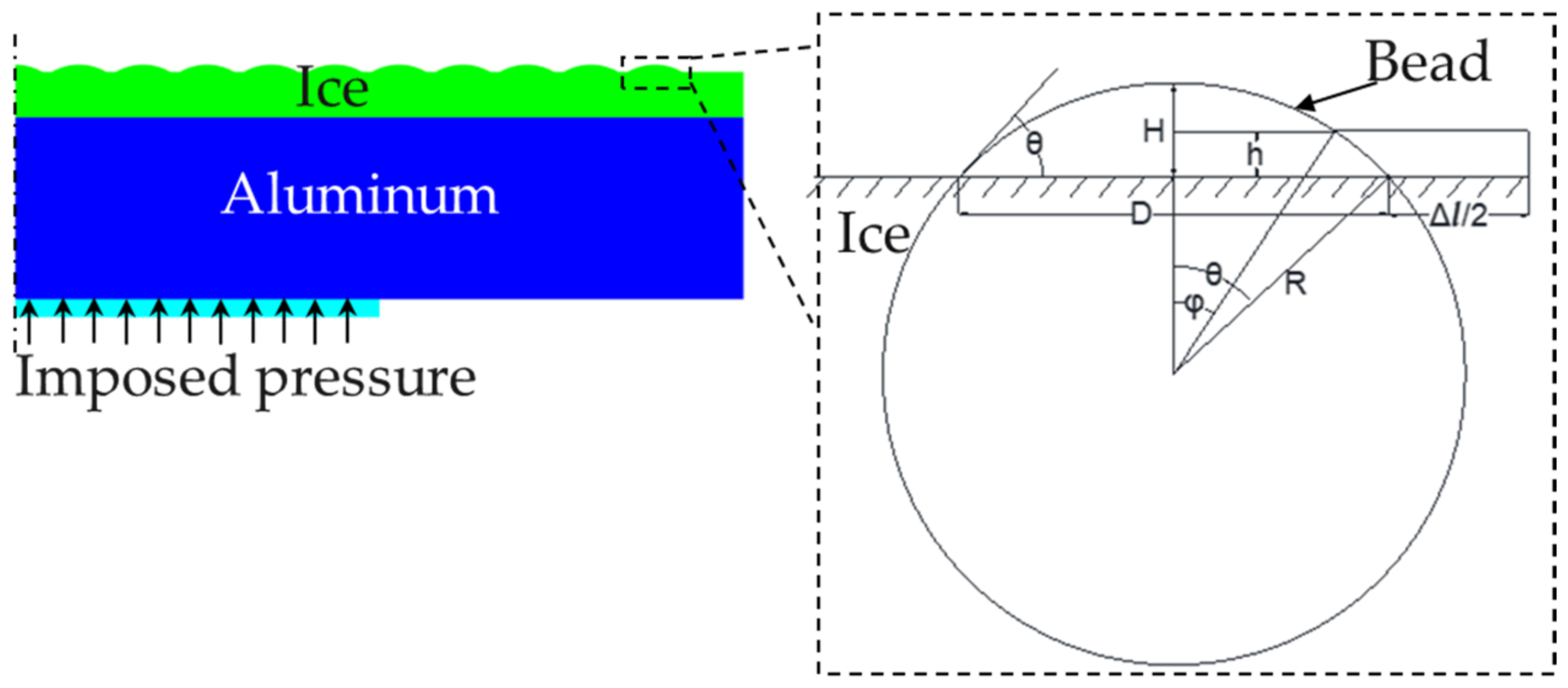
2.1. Description of the Numerical Model

In this paper, PZFlex, a high-fidelity finite element analysis (FEA) software package specialized for wave propagation problems, is used for a numerical simulation. The PZFlex software conducts acoustic modeling and simulation in the form of code input. The finite element simulation is divided into the following steps. First, define the material used in the simulation in the material’s library file and enter the material parameters. Second, input the geometric parameters in the rectangular coordinate system to build the model framework. Third, facilitate mesh generation in the established model framework. Fourth, read the material’s library file and fill the defined material in the divided mesh. Fifth, set the excitation signal. Finally, set the boundary conditions. After inputting the material parameters, geometric parameters and simulation conditions, the PZFlex finite element simulation can obtain the echo signals from interfaces. To model the pressure a transducer exerts on a solid multilayer medium, for example, we break up the layers into smaller elements. We then compute how the pressure is distributed across the layers. The overall structure of the layer is the same even though it is broken up into smaller elements. PZFlex calculates the stresses and strains on a single element. It then transfers these stresses and strains proportionally to the surrounding elements.

To study the evolution of initial small-scale ice roughness using the ultrasonic pulse-echo technique, a simplified 2-D symmetrical finite element model is established, as shown in Figure 1. The model is made up of four parts: an aluminum substrate, an ice layer, small-scale roughness profiles, and a pressure-loading area. Aluminum 7075, with a thickness of 2 mm, is chosen as the substrate. The ice layer, with a thickness 0.5 mm, is initially attached to the upper surface of the substrate. The width of the load application area shall be less than the width of the structure [30]. Since the transducer diameter used in this paper is 8 mm, both the width of the ice layer and the substrate layer can be set to twice the width of the signal-loading area, which is 16 mm. The surface profile of the ice layer is set using a bead model [2,7], and the arithmetical mean roughness value Ra is regulated by changing the radius and contact angle of the beads. All the media are assumed to have homogeneous isotropic mechanical properties. The material properties used in the simulations are shown in

Table 1. Material properties.

Material	Mass Density $\mathit{\rho }$, kg m−3	Longitudinal Velocity ${\mathit{v}}_{\mathit{p}}$, m s−1	Shear Velocity ${\mathit{v}}_{\mathit{s}}$, m s−1	Data Source
Aluminum	2690	6297.4	3172.1	Senthil et al. [31]
Ice	917.6	3713.4	1869.3	Pounder [32]

.

At the initial time, the surface coverage of the roughness element is zero, and it then rapidly reaches 85% and remains constant [2]. It is assumed that the surface coverage area of ice beads, $b=D/(D+\Delta L)$, is 85%. Note that in the bead surface profiles, we have $H=R\left(1-\cos \theta \right)$ and $\phi =\mathrm{arcos}(\cos \theta +h/R)$, where R is the cap radius, h is the height of the roughness profile’s centerline with the notations of Figure 1, and $\phi$ is the included angle of the centerline. The arithmetical mean roughness value $Ra$ can be calculated from the contact angle $\theta$ and the bead height $H$ as follows [33]:

$$Ra=\frac{bH\left(\phi -\frac{1}{2}sin2\phi \right)}{sin\theta \left(1-cos\theta \right)}$$

(1)

where $b=0.85$ is the surface coverage of the roughness elements.

To model the roughness profiles on the ice layer, at least one complete ice bead needs to be considered within the coverage of the sensor. In this numerical model, the height of the beads varies in the range of [0, 500] μm, with a sampling distance of 10 μm used to simulate the small-scale roughness of the initial surface icing. The contact angle of each bead varies in the range of [30°, 60°] in steps of 15° (the requirement for the minimum number of beads cannot be met when the contact angle is less than 30°). The value of Ra is determined by the ice cap’s height and contact angle within the model-setting range, as shown in Figure 2. The Ra’s range from 0 to 160 μm is determined mainly by the bead height within the range of simulation parameters.

2.2. Finite Element Simulation

In the present study, complete absorption boundary conditions are imposed on all boundaries except the interface between the roughness profile and air. Due to the small acoustic impedance of air, sound waves are totally reflected at the top surface of the roughness profile. The ultrasonic pulse signal source is obtained by adding a Blackman–Harris window to the sinusoidal function. The excitation source is applied at the bottom surface of the substrate with a uniform pressure. The excitation function of the pulse signal is given by:

$$\begin{array}{l}P\left(n\right)=P_{\mathrm{m}}\sin \left(3\pi \frac{n}{N-1}\right)W\left(n\right)\\ W\left(n\right)=a_0-a_1\cos \left(\frac{2\pi n}{N-1}\right)+a_2\cos \left(\frac{4\pi n}{N-1}\right)-a_3\cos \left(\frac{6\pi n}{N-1}\right)\end{array}$$

(2)

where $N$ is the sampling points of the pulse signal; $P\left(n\right)$ is the amplitude; $P_{\mathrm{m}}$ is an arbitrary constant; $W\left(n\right)$ is the Blackman–Harris window function [34], with the coefficients $a_0=0.35875$, $a_1=0.48829$, $a_2=0.14128$, and $a_3=0.01168$; and $0\le n\le N-1$.

The center frequency $f_{\mathrm{c}}$ of the pulse source is determined as $f_{\mathrm{c}}=1/T$, where $T=N\Delta t$ is the period of the ultrasonic pulse signal and $\Delta t$ is the time step of the simulation. The finite element model with 2-D symmetry is determined by a nonuniform grid technique.

The maximum frequency $f_{\mathrm{c}}$ corresponds to the minimum wavelength ${\lambda }_{\min }$, according to ${\lambda }_{\min }=v_{\mathrm{p}}/f_{\mathrm{c}}$. To ensure calculation accuracy, PZFlex requires at least 15 elements per wavelength when meshing during the simulation. As shown in Figure 3a, when the bead height is 10 μm, we can obtain echo signals with different grid sizes ranging from 1 to 10 μm. As shown in Figure 3b, when the grid size varies from 1 to 4 μm, the peak value of the echo from the top of the ice layer remains unchanged. When the grid size is greater than 4 μm, the amplitude changes greatly. Therefore, in order to ensure the accuracy of the calculation results, we set the ice layer’s grid size to 2 μm; that is, there are at least five grids at least for simulation.

The simulation is carried out with the commercial software PZFlex 2017 (Weidlinger Associates Inc., United States); the theoretical maximum stable time step for an element is $\Delta t_{\max }=\Delta x/v_{\mathrm{p},\mathrm{ice}}$, where $\Delta x=2 \mathsf{\mu }\mathrm{m}$ is the critical minimum distance across the element and $v_{\mathrm{p},\mathrm{ice}}=3713.4 \mathrm{m}/\mathrm{s}$ is the fastest wave speed of the material assigned to the element. The software automatically sets the time step according to the most critical element, $\mathrm{timestep}\le k·\Delta t_{\max }$, where $k=0.80$ is the default time step safety factor for stability. Therefore, the simulation time step is 0.4 ns, which gives a good description of the transmission of sound pressure in thin-layered media. The duration of the simulation is set to 1.5 μs.

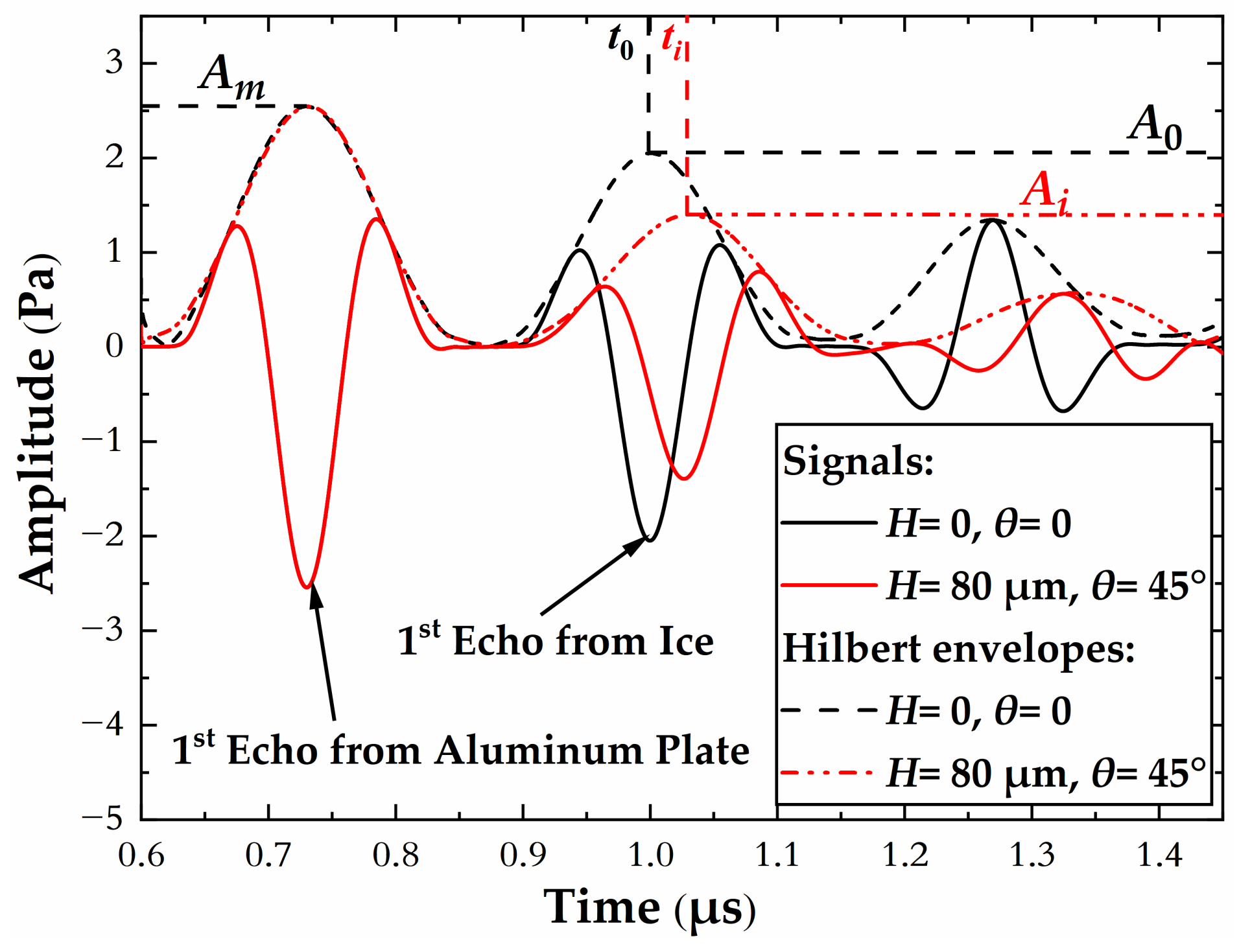
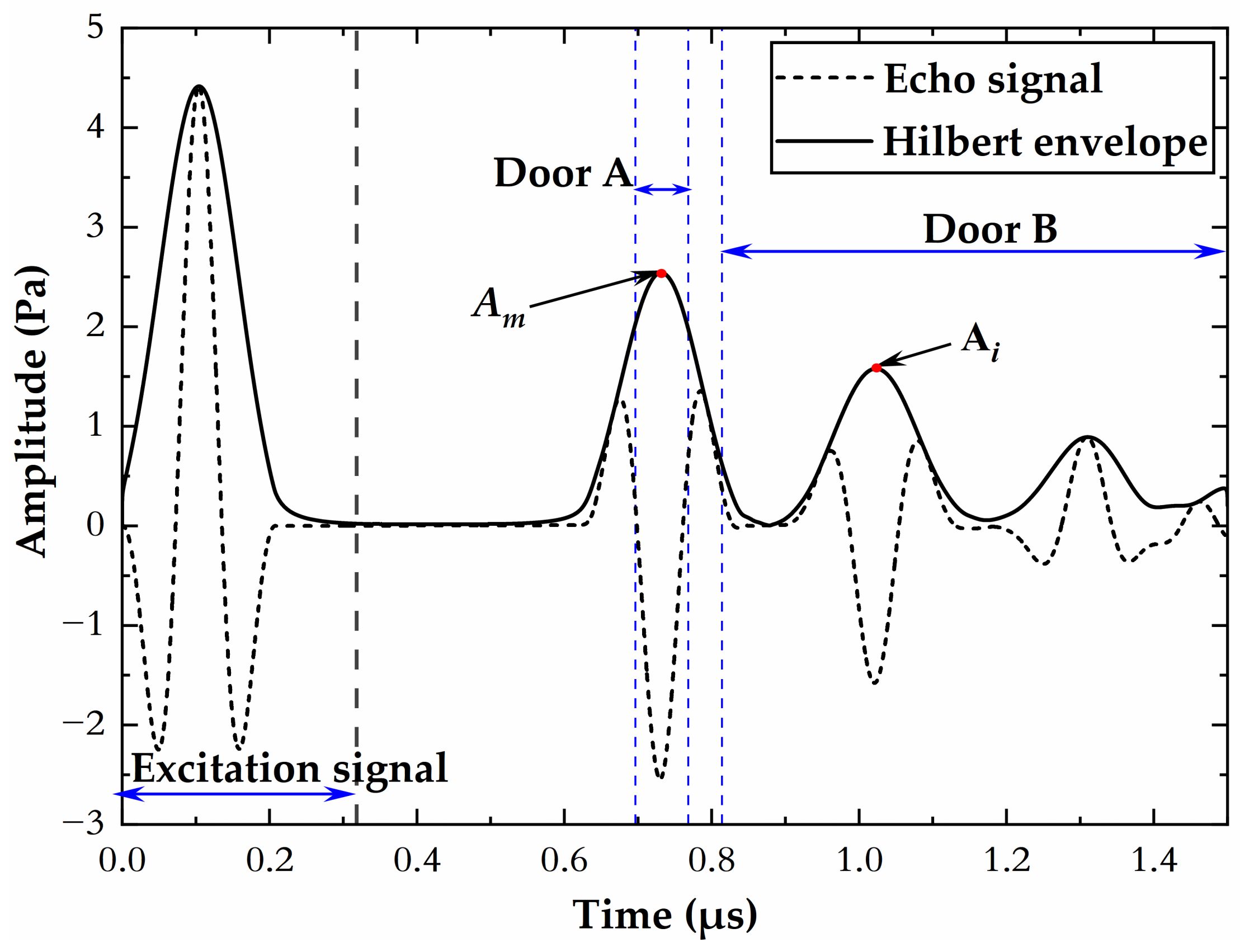
2.3. Signal Processing

The time-domain’s recorded signals are stored and then averaged by the grid nodes within the length of the excitation source. Figure 4 shows three typical pulse waves, namely, the first echo signal from the substrate–ice interface and the first and second echo signals from the top surface of the ice layer. To extract the characteristic parameters of the signals related to small-scale roughness, we perform a Hilbert transform on the time-domain signals $P(t)$ to obtain the envelopes. The thickness of the ice layer $T_{\mathrm{h}}$ is calculated from the transit time $t_{\mathrm{tof}}=t_{\mathrm{I}}-t_{\mathrm{A}}$ and longitudinal velocity $v_{\mathrm{p}}$ in the medium via $T_{\mathrm{h}}=t_{\mathrm{tof}}{v}_{\mathrm{p}}/2$, where $t_{\mathrm{A}}$ and $t_{\mathrm{I}}$ are the peak times of the envelopes from the substrate–ice interface and the top of the ice, respectively.

Ultrasonic waves propagating in a multilayer medium with different acoustic impedances will be partly transmitted and partly reflected at the interface between two adjacent layers. When a sound wave propagates from medium 1 to medium 2, the acoustic reflection coefficient $r_{1-2}$ and transmission coefficient ${\tau }_{1-2}$ are defined as follows [23]:

$$\begin{array}{l}{r}_{1-2}=\left(Z_2-Z_1\right)/\left(Z_2+Z_1\right)\\ {\tau }_{1-2}=2Z_2/(Z_2+Z_1)\end{array}$$

(3)

where $Z_1$ and $Z_2$ are the acoustic impedances of medium 1 and medium 2, respectively, given by $Z=\rho v_{\mathrm{p}}$.

In the absence of beading roughness elements, the peak amplitude of acoustic waves from the top of the ice is given by Equation (4) [23]:

$$A_0=A_{\mathrm{m}}\frac{{\tau }_{\mathrm{A}-\mathrm{I}}{r}_{\mathrm{I}-\mathrm{a}}{\tau }_{\mathrm{I}-\mathrm{A}}}{r_{\mathrm{A}-\mathrm{I}}}{\mathrm{e}}^{-2{\alpha }_{\mathrm{I}}{T}_{\mathrm{h}}}$$

(4)

where $A_{\mathrm{m}}$ is the peak acoustic amplitude from the substrate–ice interface; ${\alpha }_{\mathrm{I}}$ is the absorption attenuation coefficient of ice [23]; ${\tau }_{\mathrm{A}-\mathrm{I}}$ and ${\tau }_{\mathrm{I}-\mathrm{A}}$ are the reciprocal transmission coefficients at the substrate–ice interface; $r_{\mathrm{I}-\mathrm{a}}$ is the reflection coefficient at the ice–air interface, which is approximately equal to 1; and $r_{\mathrm{A}-\mathrm{I}}$ is the reflection coefficient at the substrate–ice interface.

For plane incident waves, the envelope peak value of echo signals from the top of the ice decreases with increasing small-scale roughness. In the present study, the reflection coefficient of the amplitude in the presence of roughness $r_i$ is given by [24]:

$$r_{\mathrm{i}}=A_{\mathrm{i}}/A_0$$

(5)

where $A_{\mathrm{i}}$ is the peak acoustic amplitude from the surface roughness.

In order to measure the ice surface roughness online, we process the echo signals from interfaces of multi-layer media with MATLAB software. As shown in Figure 5, firstly, the excitation signal is eliminated and the signal envelope is obtained, the amplitude of the primary echo from the substrate–ice interface $A_{\mathrm{m}}$ is searched globally, and Door A is set to 1/4th of the wavelength to retrieve the change in amplitude $A_{\mathrm{m}}$. Then, Door B is set between the primary and secondary echoes from the substrate–ice interface, and the amplitude of the primary echo from the ice–top interface $A_{\mathrm{i}}$ and the corresponding peak time of the ice surface in Door B are searched. The ice thickness is calculated according to the transit time and the sound velocity in the ice to determine the sound amplitude attenuation, while the echo reflection coefficient of the ice surface is determined according to the echo peak in Door B.

3. Experiment

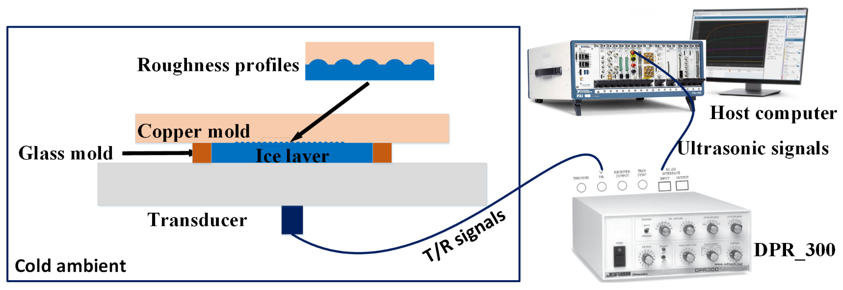
3.1. Experimental Setup

As shown schematically in Figure 6, to study the feasibility of using the UPE technique to measure the initial small-scale roughness $R_{\mathrm{a}}$ on an iced surface, an ultrasonic pulse-echo test system was built based using the LabVIEW platform. In the present study, an aluminum plate was used as the substrate with dimensions 100 mm × 100 mm × 10 mm (length × width × thickness). At −5 °C ambient temperature, an ice layer was prepared between the substrate and the copper roughness mold using a rectangular glass mold with length of 45 mm and thickness of 2 mm. An ultrasonic transducer, with center frequency of 7.5 MHz and diameter of 8 mm, was bonded to the center of the substrate bottom and connected with the ultrasonic pulser/receiver device through a coaxial cable that could effectively shield noise interference. A JSR DPR-300 pulser/receiver device (Imaginant Inc., United States), with bandwidth of 60 MHz, was used to generate and receive high-voltage pulse signals and was connected to the host computer through an RS232 serial port. Meanwhile, the pulse generator parameters (pulse amplitude, energy, repetition rate, receiver gain, high-/low-pass filter, damping, etc.) were adjusted by the host computer using the semi-customized LabVIEW software (National Instruments, United States). An NI Pxie-5114 oscilloscope board with a sampling rate of 250 MHz was used to collect the signals obtained by the JSR DPR-300 device. The received pulse-echo signals were recorded and processed on the host computer to obtain the ultrasonic time-domain and frequency-domain parameters related to the roughness.

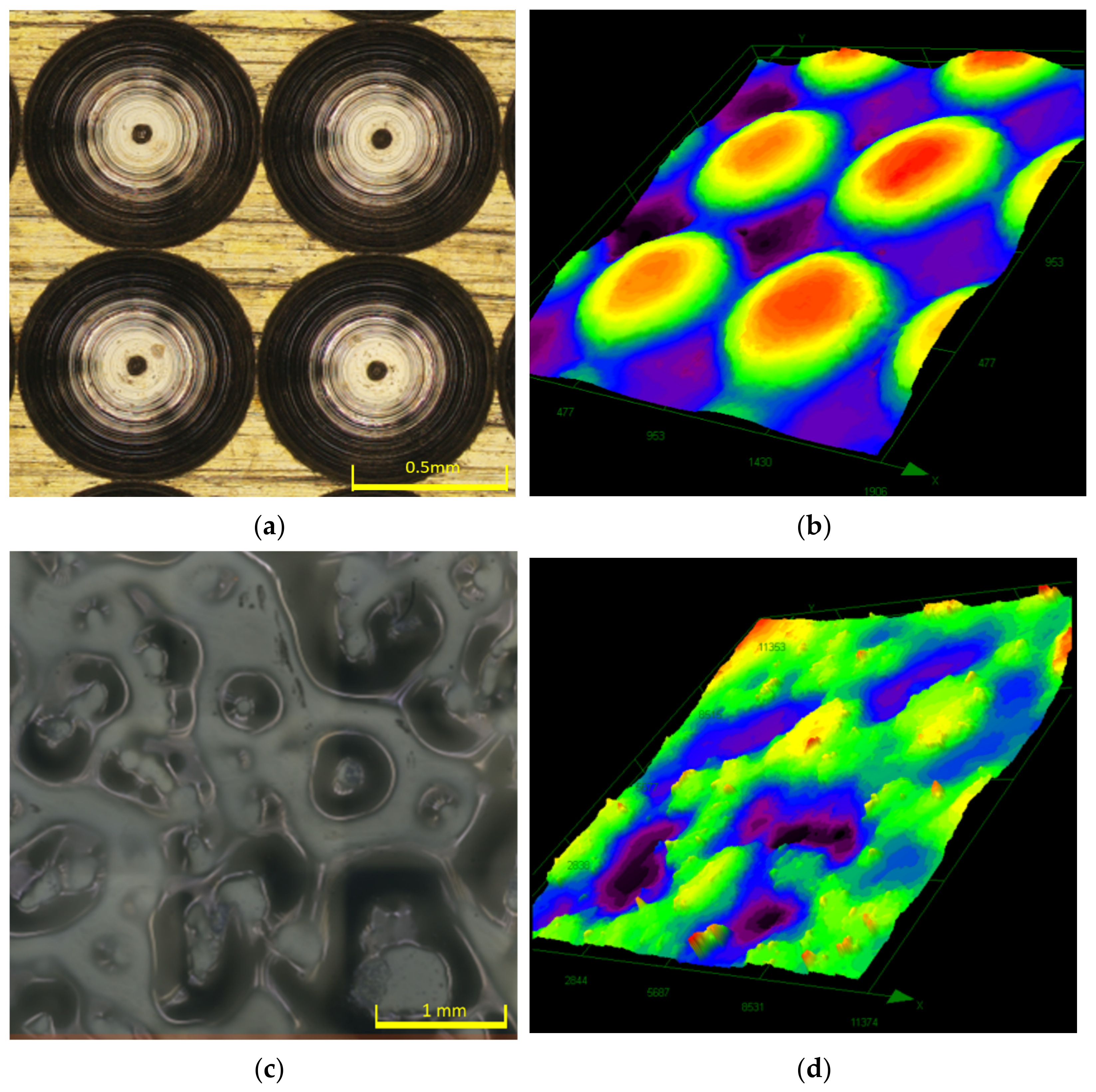
3.2. Experimental Samples

In the present study, copper molds with surface roughness ranging from 0 to 159 μm were used to effect small-scale beading roughness on the ice surface. A spherical-milling cutter with a diameter ranging from 500 to 2000 μm was used to process blind holes separated by equal intervals on the smooth copper surface, as shown in Figure 7a. To obtain a beading roughness with stable parameters, a glaze ice layer with thickness of 2 mm was first frozen at −5 °C ambient temperature in a glass container. The bead-like roughness surface was then produced by extruding the glass container between the copper mold and the substrate. As shown in Figure 7b,d, an Olympus DSX-1000 depth-of-field microscope (Olympus Corporation, Japan) was used to extract the 3-D morphology of the sample, following which the average surface roughness Sa was calculated by the corresponding software. At the same time, the UPE system collected echo signals from the interfaces.

To study the effects of roughness on ultrasonic echo signals, seventeen roughness molds with different specifications were designed, as shown in

Table 2. Roughness parameters of molds and ice surface.

Sample Number	Bead Radius R, μm	Height H, μm	Contact Angle $\mathit{\theta }$, °	2D Roughness Ra, μm	3D Roughness Sa1, μm	Measurement by Microscopic Sa2, μm
1	0	0	0	0	0	4.0
2	500	67	30	23	24	18.2
3	500	95	36	26	27	27.5
4	500	123	41	33	36	31.2
5	500	153	46	46	50	39.5
6	500	185	51	59	63	62.5
7	500	217	56	71	74	71.3
8	500	250	60	79	84	83.9
9	1250	252	37	81	85	82.5
10	1250	292	40	94	99	93.6
11	1500	287	36	92	97	96.7
12	1500	318	38	102	108	106.5
13	1750	352	37	114	120	111.3
14	1750	390	39	126	133	132.2
15	2000	424	38	137	144	140.3
16	2000	468	40	151	159	140.0
17	Irregular sample					108.8

. Sample No. 1, as the standard level of surface roughness, was prepared using a copper mold with a smooth surface. The bead-like roughness samples numbered 2–16 were prepared using copper molds with surface roughness values Sa₁ between 20 and 159 μm. To verify that the equivalent bead-like roughness model could be used to determine the influence of a rough surface on the echo signal, an additional irregular glass mold was used to prepare sample No. 17, as shown in Figure 7d. It should be emphasized that no matter what kind of ice mold is used, measurement errors will occur during the preparation of roughness samples owing to uncertainties in the freezing process. When the ice layer is frozen, it will not completely fill the pores of the mold; therefore, the roughness of the ice sample will be less than that of the mold. After demolding, when the 3-D morphology of an ice sample is scanned, owing to the time required for the measurement, water molecules from the air will freeze on the rough element’s surface to form small ice crystals, which will produce further errors in the measurement results. Therefore, in the subsequent measurements using the UPE technique, we reduce the random errors by preparing and measuring the same sample 5 times.

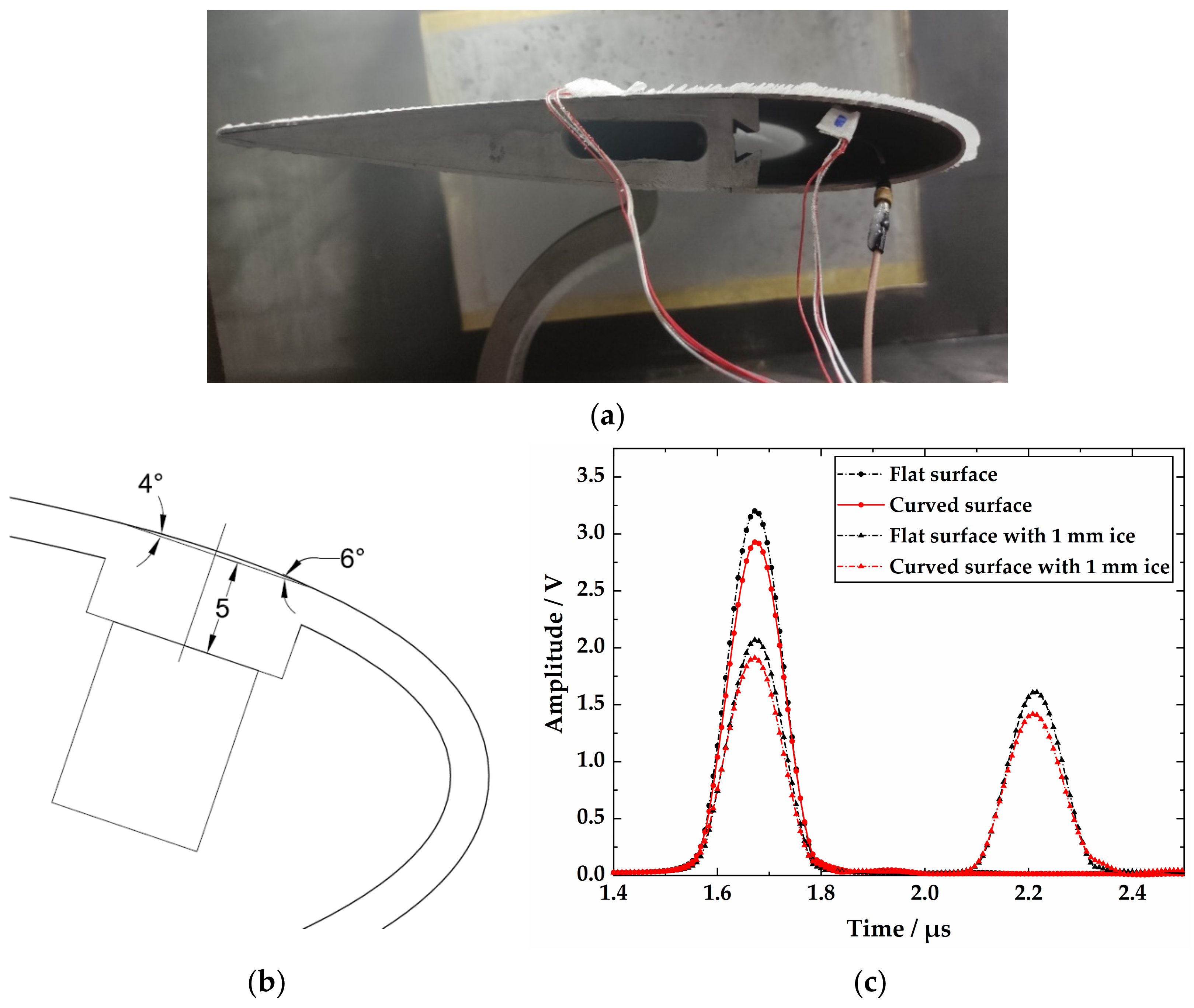
3.3. Icing Wind Tunnel Research

As shown in Figure 8a, the roughness measurement experiments were carried out in the Icing Research Tunnel at Nanjing University of Aeronautics and Astronautics (i.e., IRT-NUAA). IRT-NUAA has a test section of 0.5 m in length × 0.4 m in width × 0.3 m in height. A straight, 0.33 m chorded NACA 0012 airfoil, which spanned the entire 0.3 m test section, was used for the study. The leading edge of the airfoil was made of 7075 aluminum. The attack angle of the test airfoil was set to −5° for all cases.

As shown in Figure 8b, an ultrasonic transducer was arranged at a position 14 mm away from the stagnation point of the leading edge. The surface ice layer in this area transitioned from being smooth to rough [28]. In order to facilitate installation, the inner surface of the airfoil was flat. The structural thickness of the zone where the transducer was arranged was 5 mm.

As shown in Figure 8c, compared with the echo signal envelopes with and without an ice layer on the flat surface, when the transducer was arranged on the inner surface of the airfoil model, the echo signals from the structure–ice interface and the top of the ice layer had a certain degree of attenuation. When measuring the ice roughness, the theoretical echo peak $A_0$ from the smooth ice surface was obtained by the echo peak $A_{\mathrm{m}}$ from the substrate–ice interface and the ice thickness $T_{\mathrm{h}}$. Therefore, the radius of curvature of the airfoil surface in the transducer installation area did not affect the measurement results.

Table 3. Test conditions for roughness measurement.

Case Number	Freestream Velocity, V (m/s)	Total Temperature ${\mathit{T}}_{\mathbf{total}}$ (°C)
Case 1	24.8	−5.4
Case 2	33.0	−6.8
Case 3	41.2	−5.5
Case 4	49.5	−4.7

shows the test conditions of four cases of roughness measurement. In all of the experimental cases, the liquid water content (LWC) was set at 0.8 g/m³, and the median volumetric diameter (MVD) was set at 25 μm. The incoming airflow velocity was set at V = 24~50 m/s to study the effect of different accretion rates on surface roughness. In particular, the incoming airflow temperature was set at around −5 °C, which is a typical glaze ice condition. The duration of all four cases was 195 s. In this paper, the wind tunnel tests were mainly used to study the time-varying rule of the surface roughness of glaze ice at the same location when the freestream velocity is different.

3.4. Experimental Data Collection

To obtain the surface roughness during the initial phase of icing accretion, a transducer with center frequency of 7.5 MHz was chosen to characterize the samples with surface roughness in the range of 20–140 μm. Ultrasonic testing was carried out on the ice samples using a negative spike pulse generated by the JSR DPR-300 device with a bandwidth of 60 MHz. The echo waves were collected using an NI Pxie-5114 oscilloscope board (National Instruments, United States) with a sampling rate of 250 MS/s, as shown in Figure 9a. There are about 70 sampling points for a 7.5 MHz pulse waveform, as shown in Figure 9b. The system collects 8 groups of echo data per second to obtain dynamic measurements of ice thickness and surface roughness.

4. Results and Discussion

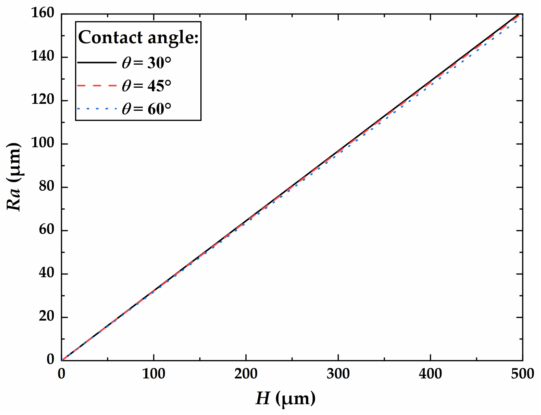
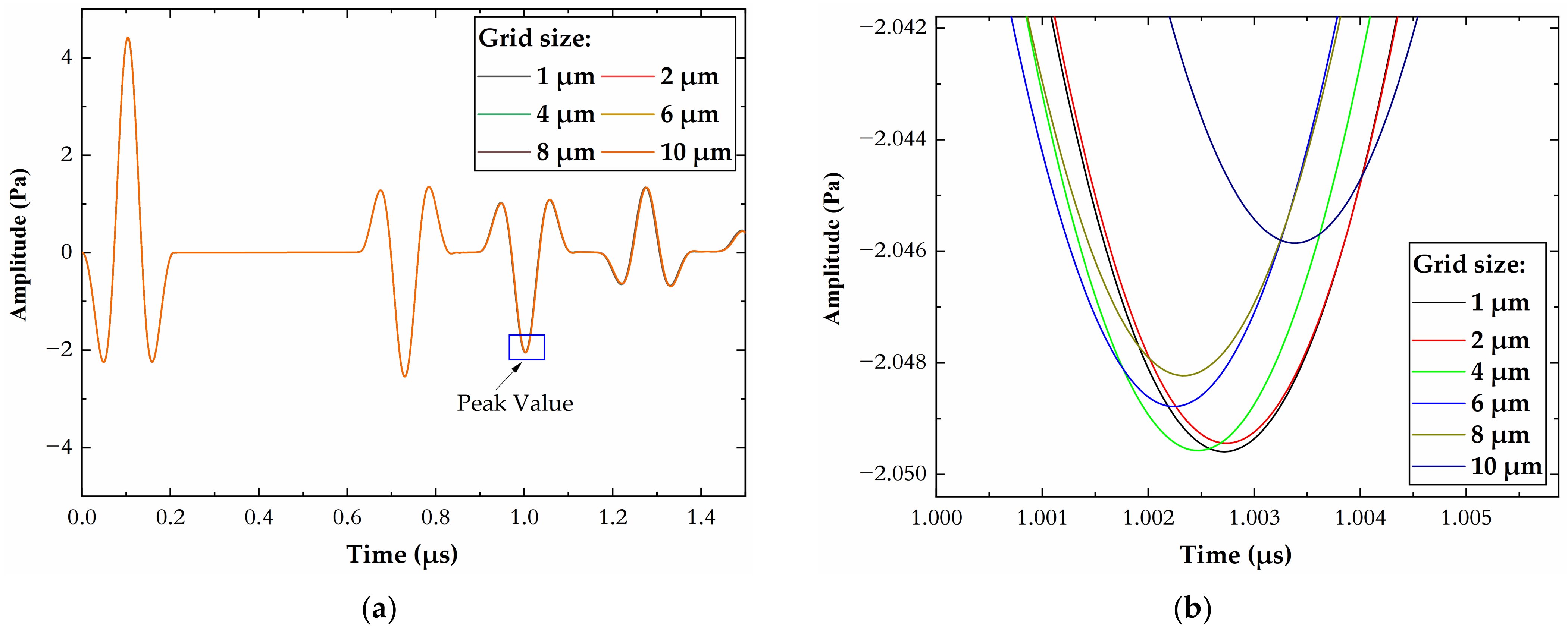
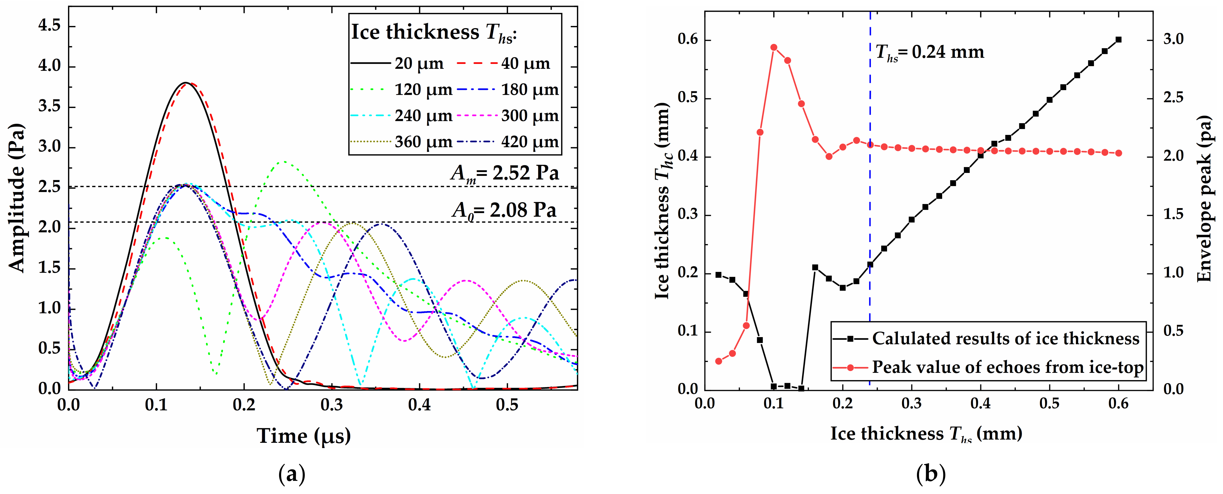
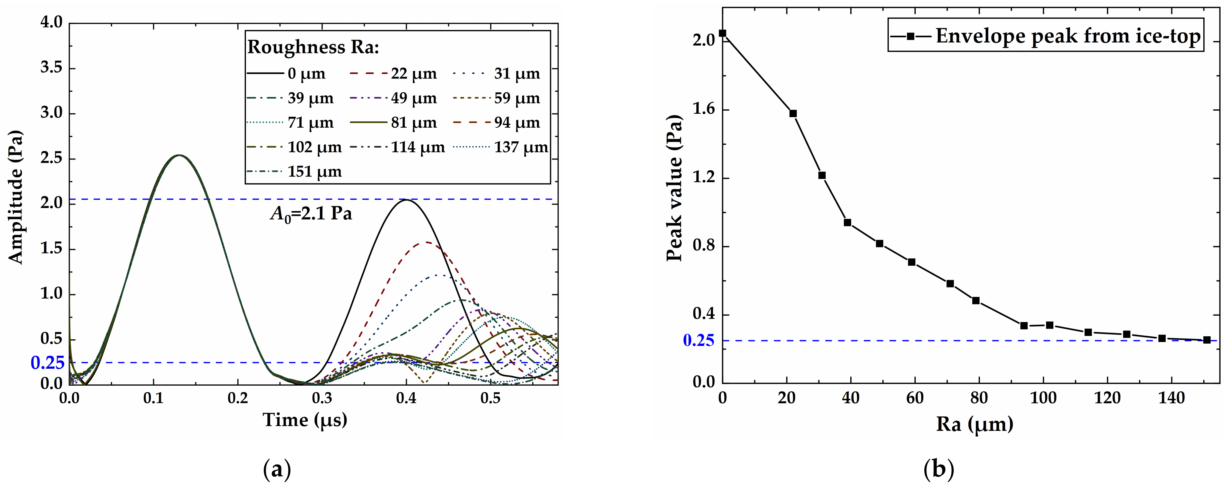
4.1. Measurement Sensitivity of Thickness and Roughness

When UPE techniques are used to detect the thickness of a thin layer, the reflected echoes from the top and bottom interfaces of the thin layer will become overlapped, which creates a difficult pattern recognition problem [35]. A direct way to overcome this problem is to use transducers with high frequency and wideband capabilities, which can enhance the resolution between echoes using a narrower pulse width [36]. However, higher frequencies will increase the sound attenuation inside the material, which will reduce the transmission distance of sound waves [23]. In the present paper, the ice thickness was measured by the UPE technique using a transducer with a center frequency of 7.5 MHz. For a thin ice layer, especially in the initial stage of the icing process, the echo signals from the top of the ice and from the substrate–ice interface will overlap, as shown in Figure 10a. To characterize the roughness by the characteristic parameters of echo envelopes, the echo signals from the top of the ice need to be stable in the absence of roughness elements.

In order to obtain the minimum ice thickness allowed by the roughness measurement, we numerically simulated the echo signals from the top of the flat ice when the thickness of the thin ice layer varies from 0 to 0.42 mm. The simulation results show that the amplitude A₀ tends to be stable during the increase in ice thickness. The echo amplitude from the substrate–ice interface remains constant when the ice thickness is in the range of [0, 0.04] mm. The echo signals from the top of the ice and the substrate–ice interface overlap strongly when the ice thickness is in the range of [0.04, 0.24] mm, which leads to the instability of the echo amplitude from the top of the ice. However, once the ice thickness becomes greater than 0.24 mm, the amplitude of the echo envelope from the top of the ice tends to be stable.

As shown in Figure 10b, when the thickness of the ice layer is greater than 0.24 mm, the peak echo from the top of the ice will decrease slightly with the increasing thickness owing to ultrasonic attenuation. Considering the frequency-dependent ultrasonic attenuation coefficient of the ice layer [23], when the thickness of the ice layer is 0.24 mm, the theoretical echo peak from a smooth surface can be calculated from Equation (4) as 2.073 Pa, which is consistent with the simulation result of 2.08 Pa. The relative error between the calculated ice thickness $T_{\mathrm{hc}}$ and the simulated design value $T_{\mathrm{hs}}$ is less than 0.3% when the ice thickness is greater than 0.24 mm. The error in the ice thickness measured by the UPE technique is much less than that measured by DIP, which is 2% [19]. Therefore, through the signal-processing methods employed in this paper, the sensitivity attained for the ice thickness measurement is 0.24 mm using a transducer with a 7.5 MHz center frequency.

The UPE technique has better sensitivity for small-scale roughness. To study the measurement range for ice roughness, the ice thickness is set to 0.5 mm; the bead contact angle and the height variation are shown in Table 2. As shown in Figure 11a, the echoes from the top of the ice would change when the surface roughness increased between 0 and 150 μm. In the same way as the time delay caused by the increase in ice thickness, the increase in the roughness element’s height will also increase the transit time of the pulse signal in the ice layer. As the rough element’s height and smooth ice thickness are components of ice thickness, we do not need to divide the time delay caused by them. As shown in Figure 11b, when the roughness Ra varied from 0 to 120 μm, there was a linear relationship between roughness and the amplitude peak value, which could be used to characterize the roughness. When the ice surface roughness was greater than 120 μm, the amplitude peak tended to be a stable value of 0.25 Pa. When the roughness increased, the echo peak value from the top of the ice was reduced from 2.1 Pa to 0.25 Pa, with the maximum reduction in the reflection coefficient being 88% according to Equation (5).

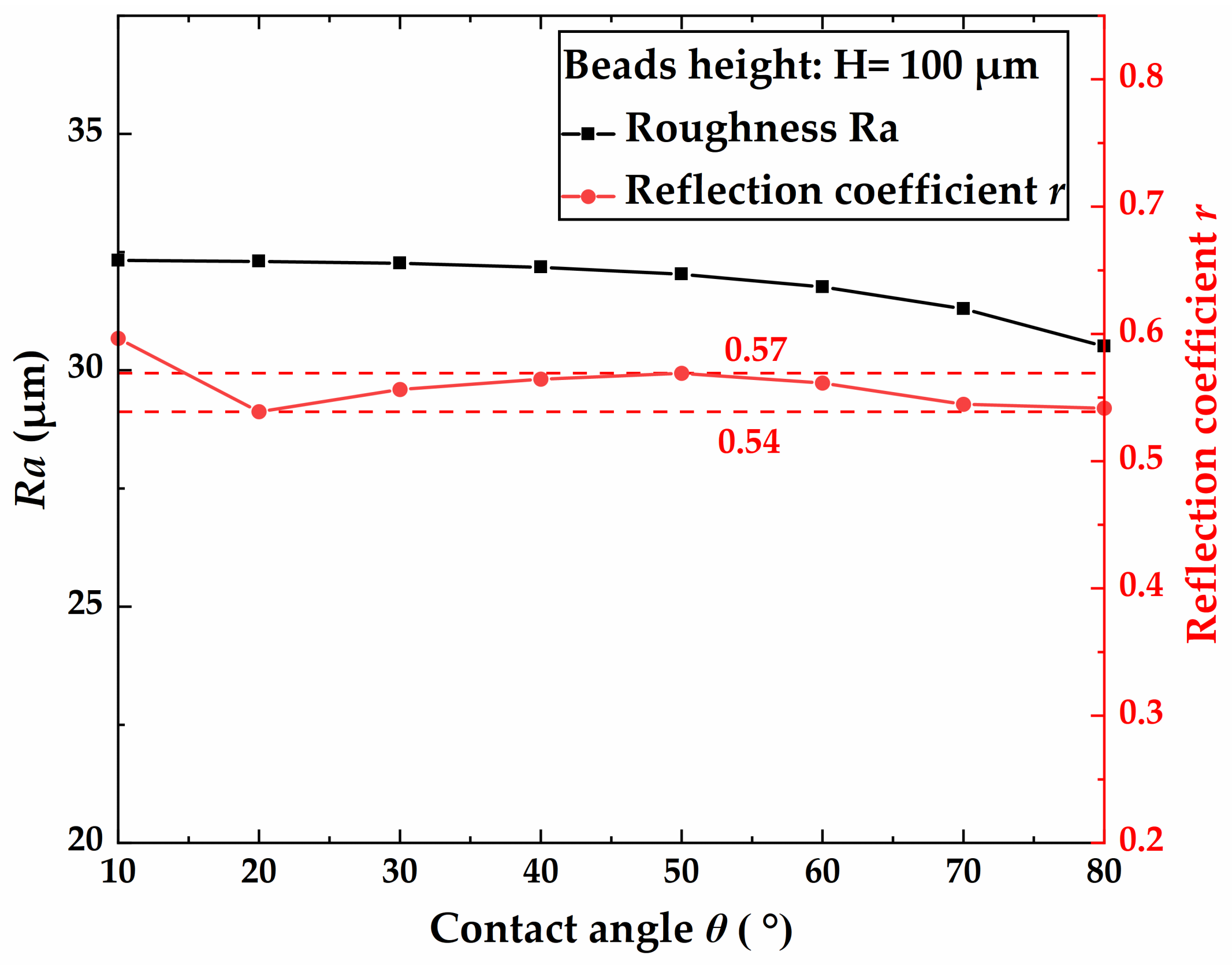
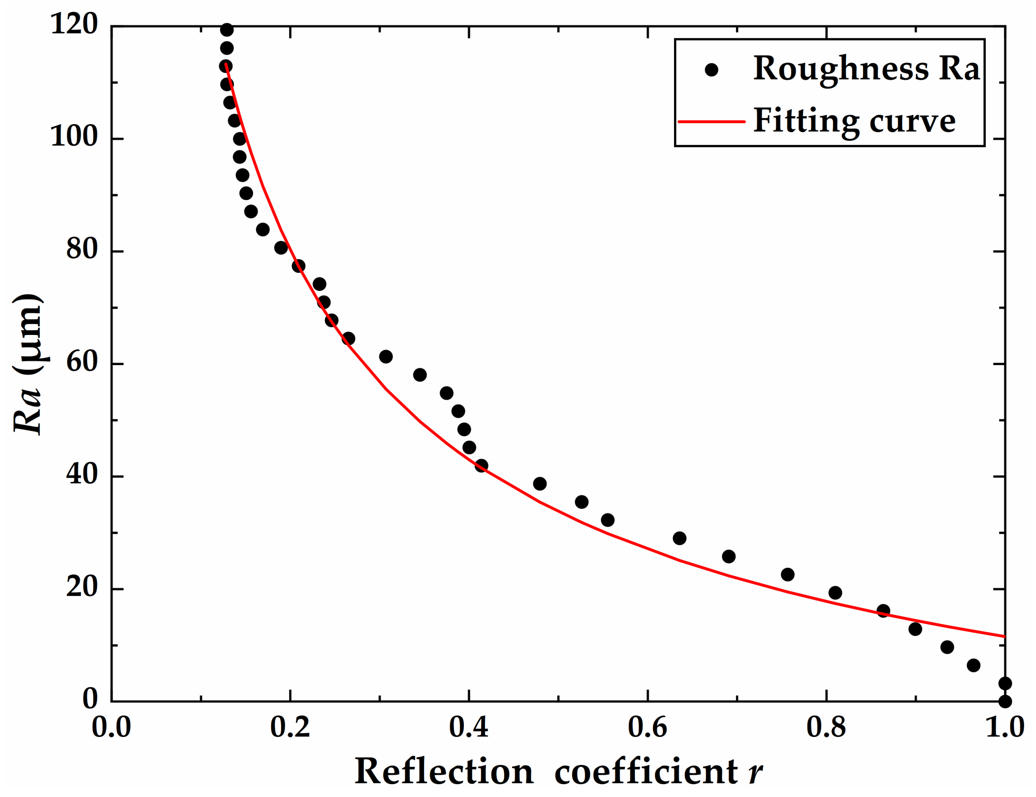
4.2. Effects of Ice Roughness on Ultrasonic Wave Propagation

In this paper, we obtain the average value of the reflected echoes from roughness elements in a certain area using the UPE technique. Figure 12 shows the effect of the bead contact angle on the reflection coefficient under the condition H = 100 μm. It is clearly seen that when the contact angle increases, the roughness value decreases slightly, according to Equation (1). When the contact angle is 10°, there is only one complete bead in the signal coverage area of the model, which will lead to a calculation error. When the contact angle changes from 10° to 20°, the simulation error will cause a sudden drop in the reflection coefficient. The reflection coefficient of the echoes from the top of the ice fluctuates within 0.03 when the contact angle is set in the range of [20, 80]°.

The roughness of an ice surface is widely investigated as the main parameter affecting the convective heat transfer coefficient of ice surfaces [9]. The relevant experimental research focuses on the measurement of the change in the height of the roughness [9,10,11], which means that it is unnecessary to decouple the influence of the height and contact angle of the beads on the reflection coefficient of the echo. The simulation results show that the echo reflection coefficient of the ice surface is insensitive to the contact angle of the rough element. The roughness value is mainly adjusted by changing the bead height, so the contact angle of the beads in the simulation model can be set as a constant value, namely, 30°. When the contact angle is set to 30°, the reflection coefficient is 0.555, which can be used to adequately simulate the average reflection coefficient and reduce the error caused by the change in the contact angle.

In order to achieve high sensitivity in an ice thickness measurement, the center frequency usually has to be greater than 5 MHz when the UPE technique is used [22]. In the present study, an ultrasonic sensor with a center frequency of 7.5 MHz has been selected, which can meet the needs of both sensitivity in the ice thickness measurement and of measuring small-scale roughness.

In the simulation, the height changes from 0 to 370 μm, and the modelled results of the changes in the ice surface roughness from 0 to 120 μm are obtained. As shown in Figure 13, the numerical results show that the echo reflection coefficient decreases with the increase in surface roughness. The red solid line is the fitting curve between roughness and the echo reflection coefficient. We can obtain the degree of roughness through the reflection coefficient according to fitting Equation (6):

$$Ra=46.48r^{-0.5637}-34.91$$

(6)

where the reflection coefficient r ranges from 0.13 to 1, and the corresponding roughness Ra varies from 11.6 to 120 μm

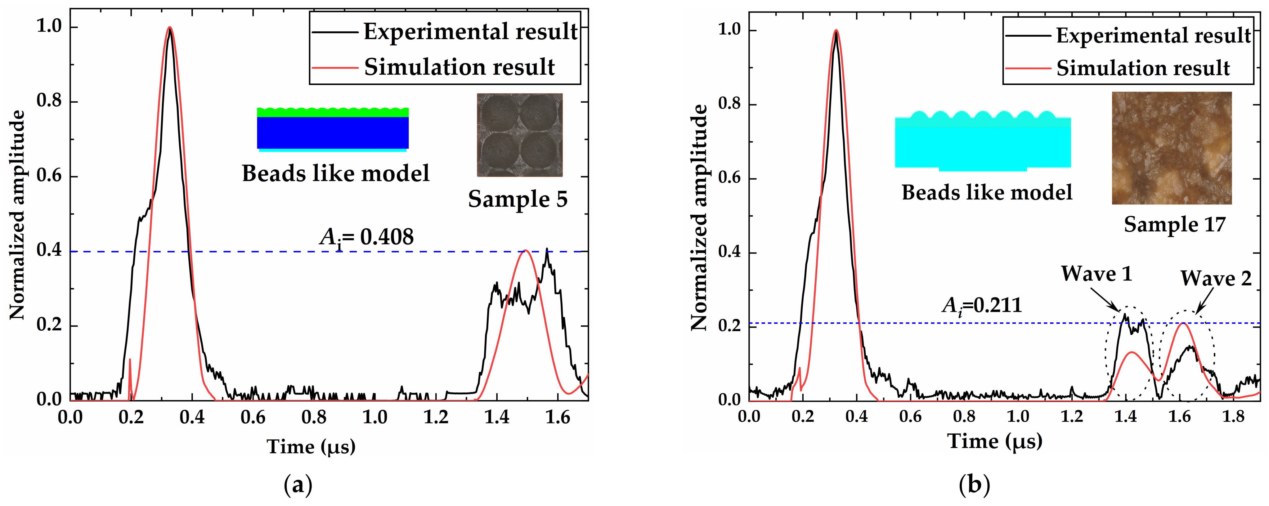
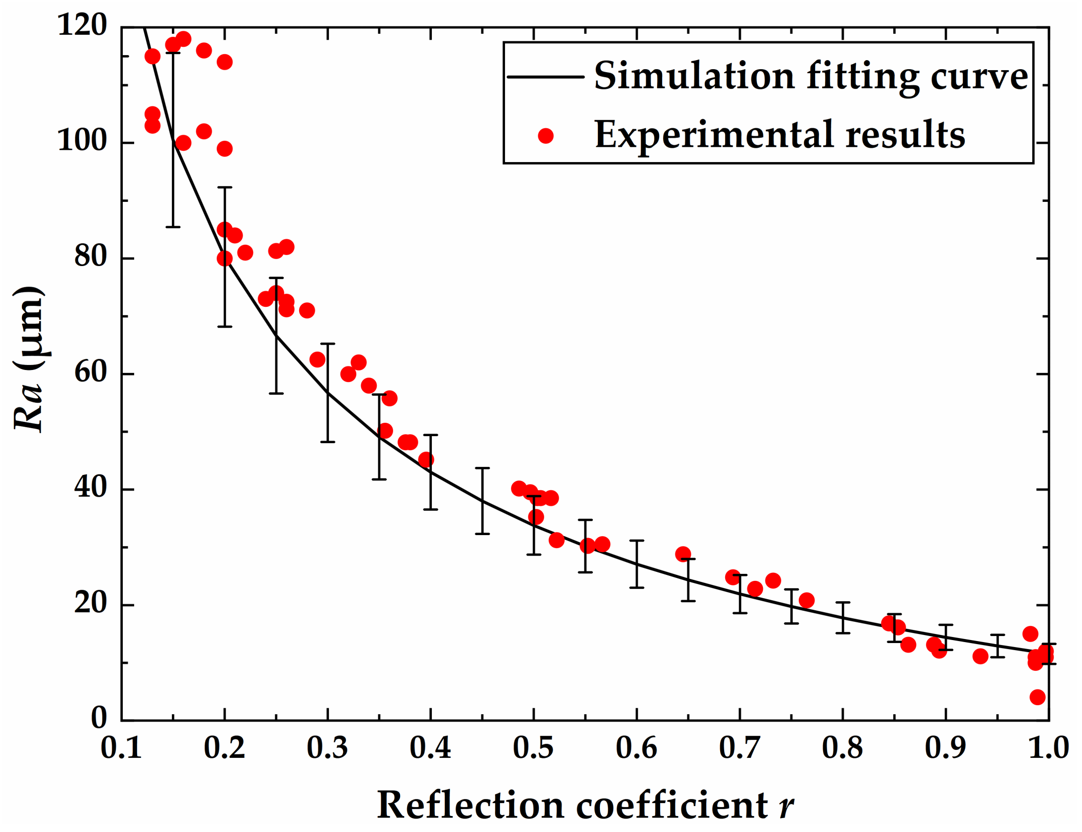
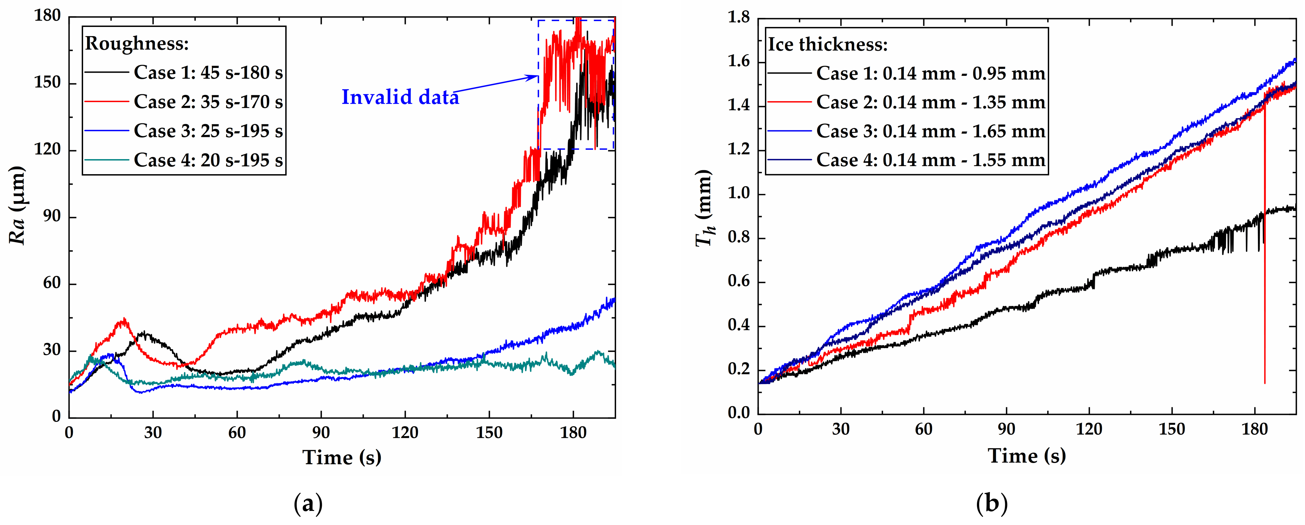
4.3. Experimental Results and Discussion

In this paper, the changes in echo signals caused by the roughness of the ice surface have been measured using an ultrasonic testing platform with ice samples produced in regular and irregular roughness molds. The envelopes of the simulated and experimental echo signals with regular bead-like roughness profiles are shown in Figure 14a. The actual surface roughness Sa of ice sample No. 5 was measured by a microscope and found to be 39.5 μm. The ice roughness value from the simulation is 38.5 μm. Upon comparing the experimental and simulated results, it is obvious that there is little difference between the echo amplitudes from the top of the ice. We can obtain a theoretical roughness of $Ra=38.5 \mathsf{\mu }\mathrm{m}$ from the amplitudes of the envelopes from the substrate–ice interface and the top of the ice according to Equations (4) and (6). Although the bead-like roughness surface prepared in the experiment was not completely and regularly distributed like the simulation model, which will distort the envelopes from the top of the ice, the envelope amplitude could still be used to identify the small-scale roughness of the ice. Figure 14b shows the normalized echo envelopes of the bead model and irregular sample No. 17 with the same roughness value. The echoes from the top of the ice are separated into two wave packets, with wave 1 and wave 2 coming from the top and bottom of the roughness profile, respectively. Although the amplitudes of wave 1 and wave 2 are different, the maximum value is 0.211, which is the echo amplitude from the top of the ice layer. Therefore, we can still use the reflection coefficient of the echo from the ice–air interface to quantitatively characterize the irregular rough surface. A comparison between the simulated and experimental waveforms shows that for irregular rough surfaces, the echo amplitude from the top of the ice is in good agreement when using the bead model for simulation.

According to Figure 11b, when the ultrasonic attenuation in the ice is not considered and the roughness is greater than 120 μm, the echo amplitudes remain unchanged. Therefore, we used ice molds No. 1–13 to prepare ice surface roughness values from 0 to 120 μm, as shown in Table 2. The damage in the ice samples caused by demolding in ground experiments will cause a 5% error in roughness. In order to reduce random errors, each copper mold was used five times to prepare ice roughness samples to investigate the effects of roughness on the reflection coefficient. The roughness of the ice surface was measured by a microscope, and the corresponding echo reflection coefficient was measured by the ice detection system.

Figure 15 shows the experimental results for different values of ice roughness. It can be seen that the roughness values measured by the microscope are in good agreement with the fitting curve. The relative error in the roughness between the experiment and simulation is less than 15% when the roughness is less than 120 μm.

Figure 16 shows the experimental results of wind tunnel test case 1. The black solid line shows the growth process regarding ice thickness, and the red solid line shows the measurement results for ice surface roughness. When glazed ice is present, there will be a thin water film on the ice surface. When the water film’s thickness is less than 20 μm, it will not significantly affect the echoes from the ice surface [37]. The variation in the thickness of the water film on the ice surface will cause a maximum roughness measurement error of 2%. In the process of real-time measurement, the ambient noise generated by the wind tunnel’s operation and the signal interference caused by the thin water film on the ice surface will cause noise interference in the roughness measurement value, which is less than 5 μm. As shown in Figure 13, the signal to noise ratio (SNR) of the pulse-echo system could be calculated as $\mathrm{SNR}=10lg{\left(P_{\mathrm{Signal}}/P_{\mathrm{Noise}}\right)}^2=26 \mathrm{dB}$, where $P_{\mathrm{Signal}}=1$ is the peak value of echo, and $P_{\mathrm{Noise}}=0.05$ is the peak value of the noise [38].

As reported by Liu et al. [23], the attenuation of ultrasound in glaze/rime ice is the result of the interaction effect of different scattering and absorption mechanisms at high frequencies (e.g., $f\ge 5.0\mathrm{MHz}$). The equations of the linear regression lines formulated for the attenuation data in the glaze-like ice samples are given in Equation (7) [23]:

$$\begin{array}{l}{\alpha }_{\mathrm{glaze}}(\mathrm{Np}/\mathrm{mm})=0.002\times f_{\mathrm{c}}\left(\mathrm{MHz}\right)+0.008\\ {\alpha }_{\mathrm{rime}}(\mathrm{Np}/\mathrm{mm})=0.0067\times f_{\mathrm{c}}\left(\mathrm{MHz}\right)+0.03\end{array}$$

(7)

In the absence of beading roughness elements, the peak amplitude of acoustic waves from the top of the ice is given by Equation (8):

$$ln\frac{A_1}{A_0}={\mathrm{e}}^{-2{\alpha }_{\mathrm{I}}{T}_{\mathrm{h}}}$$

(8)

where ${\alpha }_{\mathrm{I}}$ is the absorption attenuation coefficient of ice, $T_{\mathrm{h}}$ is the thickness of the ice layer, $A_0=1$ is the peak acoustic amplitude from the top of smooth ice without absorption attenuation, and $A_1=0.05$ is the peak acoustic amplitude after 95% attenuation.

According to Equations (7) and (8), it can be calculated that when the center frequency of the pulse signal is 7.5 MHz, 65 mm thick glaze ice and 18 mm thick rime ice can be measured at most when there is no rough element to the ice’s surface.

The experimental results showed that the surface roughness could be effectively measured when the ice thickness was greater than 0.3 mm; however, the simulation results given in Figure 10 show that for the symmetrical waveform, when the ice thickness is greater than 0.24 mm, the echo amplitude of the ice surface is stable. However, because the excitation signal was generated by the pulse generator in the experiment, the waveform cannot be completely symmetrical. Therefore, when the ice thickness was less than 0.3 mm, the echo from the substrate–ice interface will affect the echo from the ice surface, which will affect the roughness measurement results. When we conduct dynamic roughness measurement, we believe that the results are reliable when the ice thickness is greater than 0.3 mm.

Figure 17a shows the roughness evolution in the detection zone of the four experimental cases. It can be seen that for cases 1 and 2 with lower freestream velocities, the roughness increased to 120 μm within 180 s because this region was a rough ice zone [10]. When the roughness exceeded the maximum measurement value by 120 μm, the roughness value could not be accurately output; that is, the blue-dotted box contained invalid measurement data. For experimental cases 3 and 4 with higher freestream velocities, the roughness growth rate was obviously small, so the ice detection area could be considered to be a smooth zone [10]. In particular, in experimental case 4, the surface roughness fluctuated within 25–30 μm.

Figure 17b shows the dynamic measurement results of the growth in ice thickness on the skin surface in the probe arrangement area. It can be seen that when the ice thickness was greater than 0.14 mm, the UPE system could measure the thickness using the transducer with a 7.5 MHz center frequency. Regarding the icing process of glaze ice, the case with the lowest freestream velocity in the four wind tunnel tests had the lowest icing rate of 0.004 mm/s. In case 4 with the highest freestream velocity in the four wind tunnel tests, the icing rate was 0.007 mm/s. For cases 2–4 with the freestream velocity ranging from 33 to 49.5 m/s, the ice thickness growth rate at the detection point was basically the same. The experimental results show that the UPE technique can be used to measure the ice thickness growth rate in the early stage under glaze ice conditions. However, for case 1 and case 2 with lower freestream velocities, the measurement error of ice thickness increases when the test lasts for 3 min. This is because the echo signal from the top of the ice layer cannot be effectively identified. The wind tunnel test results also show that the UPE technique is very effective in measuring the thickness of smooth ice, but it cannot accurately measure the thickness of ice with a certain surface roughness.

According to Equation (1), when the average contact angle is set to 30° and the roughness is 120 μm, we can calculate that the RMH is 370 μm. Compared with previous roughness measurement results [10,16], our work shows that the UPE technique has the ability to dynamically measure ice surface roughness with a smaller scale range from 11.6 to 120 μm.

5. Conclusions

To measure the small-scale roughness that forms in the initial stage of icing, a novel multilayered model employing bead-like surface roughness was introduced to simulate the reflection of ultrasound from the top of the ice. The roughness was controlled by adjusting the bead height and contact angle. Furthermore, a UPE experimental device was developed to dynamically measure both the surface roughness and the ice thickness in the icing research tunnel. The present study has shown that the bead-like roughness model can effectively represent the effects of roughness on the characteristic parameters of echo signals. The key findings of the study are as follows:

(1) The simulation results show that an ultrasonic sensor with a center frequency of 7.5 MHz can effectively measure ice thicknesses greater than 0.24 mm and small-scale roughness values in the range of [11.6, 120] μm. The echo reflection coefficient r decreases with the increase in roughness Ra.

(2) The experimental measurements of both the regular and irregular ice samples are consistent with the echo reflection coefficients simulated assuming a bead-like surface roughness.

(3) The experimental results show that the roughness values measured by a microscope are in good agreement with the simulated fitting curve. The relative error in the roughness between the experiment and the simulation is less than 15% when the roughness is less than 120 μm.

(4) The wind tunnel test results show that the UPE technique used in this paper can effectively measure the ice growth rate and surface roughness at the initial stage of icing. When the ice thickness was greater than 0.14 mm, the UPE system could measure the thickness using a transducer with a 7.5 MHz center frequency. In addition, the surface roughness could be effectively measured when the ice thickness was greater than 0.3 mm.

To the best of the authors’ knowledge, this is the first attempt to use the UPE technique to quantitatively measure ice surface roughness in real time. This study is helpful for obtaining superior results regarding the evolution of ice surface roughness in the process of ice accretion, which can be used to improve the existing calculation model of ice accretion so as to more accurately predict the phenomenon of ice accumulation. In future work, we will measure the roughness in a wider range by changing the center frequency of the transducer. At the same time, multiple transducers will be used to measure the spatial evolution of ice surface roughness.

References

1. Cao, Y.H.; Tan, W.Y.; Wu, Z.L. Aircraft icing: An ongoing threat to aviation safety. Aerosp. Sci. Technol. 2018, 75, 353–385. [Google Scholar] [CrossRef]
2. Ozcer, I.A.; Baruzzi, G.S.; Reid, T.; Habashi, W.G.; Fossati, M.; Croce, G. FENSAP-ICE: Numerical prediction of ice roughness evolution, and its effects on ice shapes. SAE Tech. Pap. 2011. [Google Scholar] [CrossRef]
3. McClain, S.T.; Vargas, M.M.; Tsao, J.-C. Ice roughness and thickness evolution on a swept NACA 0012 airfoil. In Proceedings of the 9th AIAA Atmospheric and Space Environments Conference, Denver, CO, USA, 5–9 June 2017; p. 1. [Google Scholar]
4. Huebsch, W.W.; Rothmayer, A.P. Effects of surface ice roughness on dynamic stall. J. Aircr. 2002, 39, 945–953. [Google Scholar] [CrossRef]
5. Tagawa, G.d.; Morency, F.; Beaugendre, H. CFD study of airfoil lift reduction caused by ice roughness. In Proceedings of the 2018 Applied Aerodynamics Conference, Atlanta, GA, USA, 25–29 June 2018; p. 3010. [Google Scholar]
6. Croce, G.; De Candido, E.; Habashi, W.; Aubé, M.; Baruzzi, G. FENSAP-ICE: Numerical prediction of in-flight icing roughness evolution. In Proceedings of the 1st AIAA Atmospheric and Space Environments Conference, San Antonio, TX, USA, 22–25 June 2009; p. 4126. [Google Scholar]
7. Yoon, T.; Yee, K. Correction of local collection efficiency based on roughness element concept for glaze ice simulation. J. Mech. 2020, 36, 607–622. [Google Scholar] [CrossRef]
8. Steiner, J.; Bansmer, S. Ice roughness and its impact on the ice accretion process. In Proceedings of the 8th AIAA Atmospheric and Space Environments Conference, Washington, DC, USA, 13–17 June 2016; p. 3591. [Google Scholar]
9. Han, Y.; Palacios, J. Surface roughness and heat transfer improved predictions for aircraft ice-accretion modeling. AIAA J. 2017, 55, 1318–1331. [Google Scholar] [CrossRef]
10. Shin, J. Characteristics of surface roughness associated with leading-edge ice accretion. J. Aircr. 1996, 33, 316–321. [Google Scholar] [CrossRef]
11. McClain, S.T.; Vargas, M.; Kreeger, R.E.; Tsao, J. A reevaluation of appendix c ice roughness using laser scanning. SAE Tech. Pap. 2015. [Google Scholar] [CrossRef]
12. Anderson, D.; Shin, J.; Anderson, D.; Shin, J. Characterization of ice roughness from simulated icing encounters. In Proceedings of the 35th Aerospace Sciences Meeting and Exhibit, Reno, NV, USA, 6–9 January 1997; p. 52. [Google Scholar]
13. Reehorst, A.L.; Richter, G.P. New Methods and Materials for Molding and Casting; NASA Technical Memorandum; NASA: Washington, DC, USA, 1987; p. 15.
14. Collier, P.; Dixon, L.; Fontana, D.; Payne, D.; Pearson, A. The use of close range photogrammetry for studying ice accretion on aerofoil. Photogramm. Rec. 1999, 16, 671–684. [Google Scholar] [CrossRef]
15. McKnight, R.; Palko, R.; Humes, R. In-flight photogrammetric measurement of wing ice accretions. In Proceedings of the 24th Aerospace Sciences Meeting, Reno, NV, USA, 6–9 January 1986; p. 483. [Google Scholar]
16. McClain, S.T.; Vargas, M.; Tsao, J.-C.; Broeren, A.P.; Lee, S. Ice accretion roughness measurements and modeling. In Proceedings of the 7th European Conference for Aeronautics and Space Sciences (EUCASS), Milan, Italy, 3–6 July 2017; p. 555. [Google Scholar]
17. Puffing, R.F.A.; Hassler, W.; Tramposch, A.; Peciar, M. Ice shape mapping by means of 4D-scans. In Proceedings of the SAE 2015 International Conference on Icing of Aircraft, Engines, and Structures, Prague, Czech Republic, 22–25 June 2015; p. 8. [Google Scholar]
18. Neubauer, T.; Hassler, W.; Puffing, R. Ice shape roughness assessment based on a three-dimensional self-organizing map approach. In Proceedings of the Aiaa Aviation 2020 Forum, Virtual, 15–19 June 2020; p. 2805. [Google Scholar]
19. Liu, Y.; Zhang, K.; Tian, W.; Hu, H. An experimental study to characterize the effects of initial ice roughness on the wind-driven water runback over an airfoil surface. Int. J. Multiph. Flow 2020, 126, 103254. [Google Scholar] [CrossRef]
20. Cobbold, R.S. Foundations of Biomedical Ultrasound; Oxford University Press, Inc.: New York, NY, USA, 2007; Volume 9, pp. 609–620. [Google Scholar]
21. Hansman, R.J., Jr.; Kirby, M.S. Measurement of ice accretion using ultrasonic pulse-echo techniques. J. Aircr. 1985, 22, 530–535. [Google Scholar] [CrossRef]
22. Hansman, R.J., Jr.; Kirby, M.; Lichtenfelts, F. Ultrasonic techniques for aircraft ice accretion measurement. In Proceedings of the Sensor and Measurements Techniques for Aeronautical Applications, Atlanta, GA, USA, 1 March 1990; p. 4656. [Google Scholar]
23. Liu, Y.; Bond, L.J.; Hu, H. Ultrasonic-attenuation-based technique for ice characterization pertinent to aircraft icing phenomena. AIAA J. 2017, 55, 1602–1609. [Google Scholar] [CrossRef]
24. Heriveaux, Y.; Nguyen, V.H.; Brailovski, V.; Gorny, C.; Haiat, G. Reflection of an ultrasonic wave on the bone-implant interface: Effect of the roughness parameters. J. Acous. Soc. Am. 2019, 145, 3370. [Google Scholar] [CrossRef] [Green Version]
25. Ma, Z.; Luo, Z.; Lin, L.; Krishnaswamy, S.; Lei, M. Quantitative characterization of the interfacial roughness and thickness of inhomogeneous coatings based on ultrasonic reflection coefficient phase spectrum. NDT E Int. 2019, 102, 16–25. [Google Scholar] [CrossRef]
26. Okajima, K.; Nagaoka, S.; Islam, M.R.; Ito, R.; Watanabe, K. Development and testing of a surface roughness measurement device based on aerial ultrasonic reflections. Paddy Water Environ. 2019, 18, 345–353. [Google Scholar] [CrossRef]
27. Shannon, T.A.; McClain, S.T. Convection from a simulated NACA 0012 airfoil with realistic ice accretion roughness variations. In Proceedings of the SAE International Conference on Icing of Aircraft, Engines, and Structures, Montreal, QC, Canada, 22–25 June 2015; p. 13. [Google Scholar]
28. Anderson, D.; Hentschel, D.; Ruff, G. Measurement and correlation of ice accretion roughness. In Proceedings of the 36th AIAA Aerospace Sciences Meeting and Exhibit, Reno, NV, USA, 12–15 January 1998; p. 98. [Google Scholar]
29. Zhang, K.; Liu, Y.; Rothmayer, A.P.; Hu, H. An experimental study of wind-driven water film flows over roughness array. In Proceedings of the 6th AIAA Atmospheric and Space Environments Conference, Atlanta, GA, USA, 16–20 June 2014; p. 2326. [Google Scholar]
30. Berezovski, A.; Engelbrecht, J.; Maugin, G.A. Numerical simulation of two-dimensional wave propagation in functionally graded materials. Eur. J. Mech. 2003, 22, 257–265. [Google Scholar] [CrossRef] [Green Version]
31. Senthil, K.; Iqbal, M.A.; Chandel, P.S.; Gupta, N.K. Study of the constitutive behavior of 7075-T651 aluminum alloy. Int. J. Impact Eng. 2017, 108, 171–190. [Google Scholar] [CrossRef]
32. Petrenko, V.F.; Whitworth, R.W. The Physics of Ice; Elsevier: New York, NY, USA, 1999; Volume 6. [Google Scholar]
33. Gadelmawla, E.; Koura, M.M.; Maksoud, T.M.; Elewa, I.M.; Soliman, H. Roughness parameters. J. Mater. Process. Technol. 2002, 123, 133–145. [Google Scholar] [CrossRef]
34. Harris, F.J. On the use of windows for harmonic analysis with the discrete fourier transform. Proc. IEEE 1978, 66, 51–83. [Google Scholar] [CrossRef]
35. Al-Aufi, Y.A.; Hewakandamby, B.N.; Dimitrakis, G.; Holmes, M.; Hasan, A.; Watson, N.J. Thin film thickness measurements in two phase annular flows using ultrasonic pulse echo techniques. Flow Meas. Instrum. 2019, 66, 67–78. [Google Scholar] [CrossRef]
36. Shpigler, A.; Mor, E.; Bar-Hillel, A. Detection of overlapping ultrasonic echoes with deep neural networks. Ultrasonics 2022, 119, 106598. [Google Scholar] [CrossRef]
37. Wang, Y.; Wang, Y.; Li, W.; Wu, D.; Zhao, N.; Zhu, C. Study on freezing characteristics of the surface water film over glaze ice by using an ultrasonic pulse-echo technique. Ultrasonics 2022, 126, 106804. [Google Scholar] [CrossRef]
38. Madu, I.E.; Madu, C.N. Design optimization using signal-to-noise ratio. Simul. Pract. Theory 1999, 7, 349–372. [Google Scholar] [CrossRef]
Figure 1. Schematic of a simplified 2-D symmetrical finite element model with bead-like roughness on an ice surface.
Aerospace 09 00739 g001
Figure 2. Variation in roughness with bead height at different contact angles.
Aerospace 09 00739 g002
Figure 3. Simulation results of different grid sizes when the bead height is 10 μm: (a) Echo signals. (b) Partial enlarged view of reflected wave at the top of ice layer.
Aerospace 09 00739 g003
Figure 4. Radiofrequency echo signals (solid lines) with their envelopes (dashed lines) for an ice layer of thickness 0.5 mm. The black lines are for standard signals without roughness profiles, and the red lines are for a roughness height and a contact angle of 80 μm and 45°, respectively.
Aerospace 09 00739 g004
Figure 5. The original pulse-echo signal and its envelope at the interface of multilayer media.
Aerospace 09 00739 g005
Figure 6. Experimental setup for measurement of roughness Ra via UPE method.
Aerospace 09 00739 g006
Figure 7. Small-scale ice roughness samples and copper molds measured by Olympus DSX-1000 microscope: (a) copper mold with spherical holes; (b) the three-dimensional contours of the regular bead ice sample; (c) glass mold with irregular roughness profile; (d) the three-dimensional contours of the irregular surface ice sample.
Aerospace 09 00739 g007
Figure 8. Installation of the ultrasonic transducer on NACA0012 airfoil model: (a) airfoil model in the icing wind tunnel, (b) schematic diagram of the transducer’s installation position, and (c) the envelopes of echoes.
Aerospace 09 00739 g008
Figure 9. Data obtained from test with surface roughness of Sa = 40 μm. The pulse in the dot-dashed rectangle is the first echo from the substrate–ice interface, and the pulse in the solid rectangle is the first echo from the top of the ice. (a) Experimental echo waveform. (b) Waveform from top of ice.
Aerospace 09 00739 g009
Figure 10. Simulation results for echo envelopes from a smooth ice top: (a) echo envelopes for different ice thicknesses; (b) ice thickness and envelope peak.
Aerospace 09 00739 g010
Figure 11. Simulation results for echo envelopes with roughness varying from 0 to 151 μm: (a) Echo envelopes; (b) peak value.
Aerospace 09 00739 g011
Figure 12. Numerical simulation results of roughness Ra and reflection coefficient r vs. contact angle.
Aerospace 09 00739 g012
Figure 13. Corresponding relationship between roughness Ra and echo reflection coefficient r; beads’ contact angle is 30° and beads’ height is in the range of [0, 370] μm.
Aerospace 09 00739 g013
Figure 14. Comparison between experimental and simulated envelopes of echo signals: (a) echoes from top of ice with regular bead profile and with Ra = 38.5 μm and Sa = 39.5 μm; (b) echoes from bead-like profile with Ra = 108 μm and irregular roughness profile with Sa = 108.8 μm.
Aerospace 09 00739 g014
Figure 15. Experimental results for ice surface roughness in the range of [0, 120] μm.
Aerospace 09 00739 g015
Figure 16. The experimental results of case 1, where the black solid line is the growth process of ice thickness, and the red solid line is the variation in ice surface roughness.
Aerospace 09 00739 g016
Figure 17. Experimental results from the icing research tunnel: (a) the growth process of the ice layer, and (b) the variation in surface roughness on the ice layer.
Aerospace 09 00739 g017