Model Predictive Control Based on ILQR for Tilt-Propulsion UAV

Abstract

The transition flight of tilt-propulsion UAV is a complex and time-varying process, which leads to great challenges in the design of a stable and robust controller. This work presents a unified model predictive controller, which can handle the full envelope from vertical take-off and landing to cruise flight, to mean that the UAV can achieve a near-optimal transition flight under uncertainty conditions. Firstly, the nonlinear dynamic model of the tilt-propulsion UAV is developed, in which the aerodynamic/propulsion coupling effect of the ducted propeller is considered. Then, a control framework, including global trajectory planning and finite horizon control, is designed. Taking the planned global trajectory as the reference input, a controller is proposed with an inner layer based on ILQR optimization and an outer layer based on feedback correction and forward rolling of the MPC frame. The ILQR-MPC controller has high computational efficiency to deal with nonlinear problems, and has the ability to give full play to UAV’s control ability and suppress uncertainty. Finally, the simulation results show that ILQR-MPC controller obviously performs better than the ILQR feedforward controller, and gains a scheduling PID controller and MPC controller.

1. Introduction

Vertical take-off and landing (VTOL) aircraft have two outstanding advantages: flexible take-off and landing, without the requirement for airport conditions, and a long endurance with high-speed cruise ability. In terms of military use, it could be used for mountain battle and VTOL from ships, while more and more VTOL urban aircrafts are gradually emerging for civil use. Therefore, based on its significant advantages and great application prospects, VTOL aircraft have attracted more attention in recent years [1,2,3,4].

VTOL aircrafts are mainly classified into tilt-rotor aircraft [5], tilt-wing aircraft [6], tilt-propulsion aircraft [7], tail-seat aircraft [8], etc. These four kinds of aircrafts realize mode transition between VTOL flight and high-speed cruise through thrust vector tilting. The transition flight is a crucial and complex process. Taking the tilt-propulsion aircraft as an example, in transition flight, the aerodynamic force of the wing rapidly changes with the airspeed, the propulsion system has a time-varying propulsion and aerodynamic characteristics, and the system has obvious uncertainty; therefore, the challenges in tilt-propulsion aircraft development are mainly the transition trajectory plan and the control scheme design of a transition flight.

As in the commercial PixHawk autopilot, the common approach to VTOL UAVs is to design two or three sub-controllers [9,10,11], in which some schemes with only the rotor controller and the fixed-wing controller realize transition flight control by combining the two controllers. In addition, many researchers [12,13] split the control problem into several control regimes and focus on a smooth switch between the individual modes.

MPC is an advanced optimal control strategy based on the receding horizon, which can handle Multi-Input Multi-Output (MIMO) and nonlinear systems, as well as switching systems with soft and hard constraints [14]. Papachristos et al. [15] applied a Linear Model Predictive Control (LMPC) by splitting the range of the unmanned quad-tiltrotors forward velocity in many subsets. Then, based on an interior-point solver, a code generator [16] was shown for the embedded implementation of a linear MPC. Nonlinear MPC has also been widely used. Quirynen et al. [17] proposed a framework for fast Nonlinear Model Predictive Control (NMPC); then, Kamel et al. [18] designed a fast attitude controller for a multicopter based on this approach. Papachristos et al. [19] proposed an explicit model predictive control scheme relying on constrained multiparametric optimization for a thrust-vectoring tri-tiltrotor, addressing the exploitation of the combined potential of the directly actuated and the underactuated control authorities. Allenspach and Ducard [20] presented an MPC controller for full-flight envelope trajectory-tracking for a convertible UAV with fixed wings and thrust vectoring. Manzoor et al. [21] addressed the trajectory tracking control problem of a Ducted Fan UAV (DFUAV) based on an offset-free Model Predictive Control (MPC) technique subject to various uncertainties and external disturbances, which ensures adequate robustness and stability in the controller. However, the use of a linear model led to control accuracy reductions in the MPC controller, so this approach may not be suitable for a highly nonlinear system. L. Bauersfeld et al. [22] proposed a control frame combining MPC and control allocation to constitute a unified nonlinear control approach for tilt-rotor VTOL aircraft, which is valid in all flight modes and transitions. The feasibility of this method was verified through simulation and outdoor experiments; however, the computation load based on nonlinear MPC is too large.

The high computational cost has long been a great challenge for MPC controllers, especially the NMPC. Therefore, it is very important to reduce the computational complexity with the high-accuracy guarantee for MPC. Differential Dynamic Programming (DDP) is a famous shooting algorithm used for numerical optimization [23], with superlinear convergence rate in the horizon length, hence its success in robotics [24]. One well-known variant of DDP, called an iterative linear quadratic regulator (ILQR), was proposed in [25], demonstrating its abilities in various simulations. Sequential research [26] has shown the feasibility of ILQR in simulations. In recent years, the ILQR-based MPC methods were gradually applied in robotics [27,28] and achieved good results.

Since the trajectory planner is required to solve a complex long-horizon optimization problem, respecting the system dynamics and constraints, it cannot react very dynamically to uncertainty. Additionally, the controller is often tracking a fixed trajectory with no authority to adjust it. The global trajectory plan based on ILQR and the finite-horizon optimal control based on ILQR-MPC are proposed in this paper for the optimal transition flight of tilt-propulsion UAV (TPUAV). It is worth mentioning that the unified flight control of the full envelope can be realized based on a single MPC controller with near linear computational complexity, which is the first application of the ILQR in the field of VTOL aircraft.

The main contribution of this work lies in the following proposals:

1. A model considering the aerodynamic/propulsion coupling characteristic of the ducted propeller is developed to improve the accuracy of dynamic model.

2. An MPC controller is proposed for flight control of the TPUAV transition process based on ILQR, which has higher control accuracy and a better ability to deal with uncertainty compared with gain scheduling PID and MPC controllers.

3. The ILQR-MPC controller is a unified controller, which can deal with the full envelope of TPUAV, from VTOL to cruise flight.

The remainder of this manuscript is organized as follows. Firstly, an introduction to tilt-propulsion UAV is presented. The dynamics model of TPUAV is developed, where emphasis is placed on the modeling of the ducted propeller. Section 3 introduces the proposed method in detail, including the global trajectory plan approach and the MPC based on ILQR. Afterwards, the results of the simulation work are shown. Lastly, Section 5 concludes the full manuscript.

2. System Model

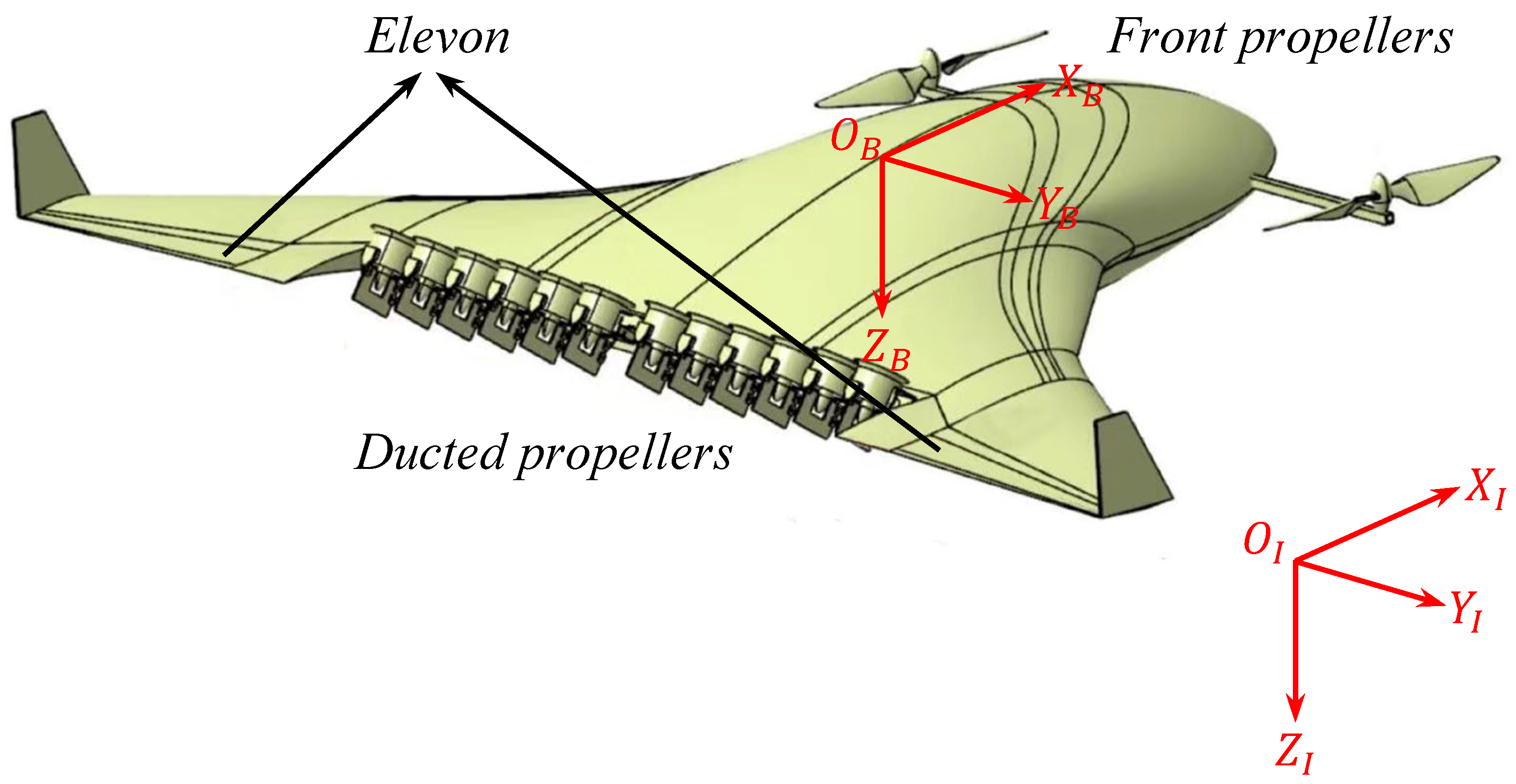
2.1. Tilt-Propulsion UAV Configuration

We designed a novel tilt-propulsion UAV with BWB configuration (shown in Figure 1), consisting of fuselage, front propellers, ducted propellers, and elevon. The front propellers, composed of a pair of propellers, are symmetrical at the X axis of the fuselage, which cannot tilt, so that they just provide a vertical thrust for UAV. The ducted propellers were installed at the rear of the fuselage, dividing the left and right groups, and the ducted propellers have the ability to change thrust direction by tilting, with a range from π⁄2 to 0.

TPUAV has a large flight envelope, including vertical takeoff and landing and high-speed cruise. Its flight modes are similar to those of a tiltrotor aircraft with rotor mode, transition mode and fixed-wing mode. In addition, there are two unique advantages of TPUAV compared with a traditional tiltrotor aircraft. On the one hand, the flexibly configured propulsion system and BWB configuration improve the lift–drag ratio as well as the aerodynamic efficiency. On the other hand, the design of the distributed propulsion system enhances the fault tolerance of the system and provides a stronger security guarantee for UAV.

2.2. Dynamic Model of TPUAV

Due to the special layout of TPUAV, the high complexity of the propulsion system, and the obvious changes in system equations during the transition process, it is necessary to develop a reliable dynamic model to achieve the global trajectory plan and high-precision control in transition flight.

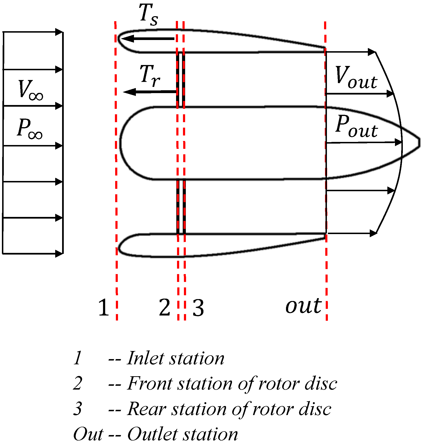
2.2.1. Aerodynamic Model of Fuselage

The elevon of TPUAV has the functions of aileron and elevator of traditional aircraft. The deflection of left surface is ${\delta }_{el}$ and the right one is ${\delta }_{er}$; then, the compound control variable could be expressed as

$$\left[\begin{array}{c}{\delta }_e\\ {\delta }_a\end{array}\right]=\left[\begin{array}{cc}\raisebox{1ex}{$1$}\!\left/ \!\raisebox{-1ex}{$2$}\right.& \raisebox{1ex}{$1$}\!\left/ \!\raisebox{-1ex}{$2$}\right.\\ -\raisebox{1ex}{$1$}\!\left/ \!\raisebox{-1ex}{$2$}\right.& \raisebox{1ex}{$1$}\!\left/ \!\raisebox{-1ex}{$2$}\right.\end{array}\right]\left[\begin{array}{c}{\delta }_{el}\\ {\delta }_{er}\end{array}\right]$$

(1)

where ${\delta }_a$ represents the equivalent deflection of aileron, while ${\delta }_e$ represents that of elevator.

The lift, drag, and pitch moment of the fuselage in the wind axis system could be expressed as

$$\left\{\begin{array}{c}{F}_x=\frac{1}{2}\rho V^{2}S\left(C_{D0}+C_{D\alpha }\alpha +C_{Dq}\frac{\overline{c}}{2V}q+C_{D{\delta }_e}{\delta }_e\right)\\ F_z=\frac{1}{2}\rho V^{2}S\left(C_{L0}+C_{L\alpha }\alpha +C_{Lq}\frac{\overline{c}}{2V}q+C_{L{\delta }_e}{\delta }_e\right)\\ M_y=\frac{1}{2}\rho V^{2}S\overline{c}\left(C_{m0}+C_{m\alpha }\alpha +C_{mq}\frac{\overline{c}}{2V}q+C_{m{\delta }_e}{\delta }_e\right)\end{array}\right.$$

(2)

where $\rho$ is the air density, $V$ is the airspeed, $S$ is the reference area of fuselage (including the traditional wing), $\alpha =\arctan \left(V_z/V_x\right)$ is the angle of attack, $\overline{c}$ is the average aerodynamic chord, $q$ is pitch angular speed, $C_L,C_D,C_M$, respectively, denote the coefficients of lift, drag and pitch moment, and the different subscripts $0,\alpha ,q,{\delta }_e$ indicate that coefficients are related to different parameters.

2.2.2. Model of Front Propellers

The rotation of front propellers produces lift as well as reverse torque. The calculation formula of thrust and torque coefficient of the front propellers are expressed as follows

$$C_{Tf}=\frac{T_f}{\rho n_f^2{D}_f^4},C_{Qf}=\frac{Q_f}{\rho n_f^2{D}_f^5}$$

(3)

where $T_f,Q_f$ represent the thrust and torque of front propellers, respectively; $n_f,D_f$ represent the rotation speed and diameter of front propellers, respectively.

The incoming flow velocity would have an impact on the coefficients of thrust and torque, in which the influence of axial flow velocity is much greater than that of radial. However, the front propeller is perpendicular to the XZ plane of airframe. In the transition process, the axial component of the incoming flow is so small to ignore; therefore, the influence of incoming flow on the front propeller could be ignored. In real flight, the neglected part of the system model is regarded as uncertainty.

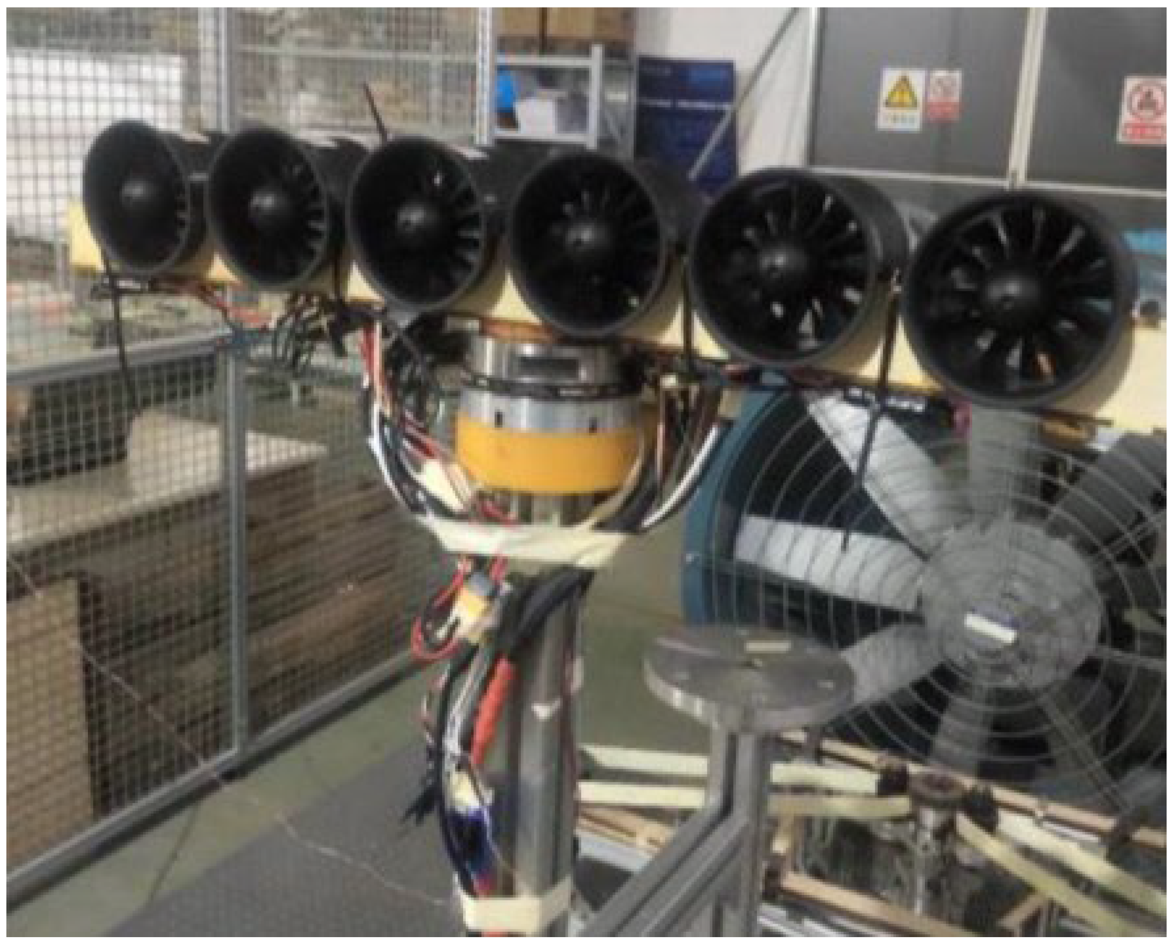
2.2.3. Model of Ducted Propellers

Compared with the isolated propeller, the external duct could provide an extra thrust when the incoming flow speed is low, so the ducted propeller has a higher propulsion efficiency. At present, the research on the isolated propeller has been quite perfect; however, for the ducted propeller, how to accurately describe the quantitative relationship between the rotor thrust and the total thrust needs to be fully explored.

The typical stations of the ducted propeller are introduced as follows: “$1,out$” respectively represent inlet station and outlet station; “$2,3$”, respectively, represent front and rear stations of the rotor disc; the subscript “$\infty$” represents the variables related to free flow state. More details about typical stations are showed in Figure 2 and the real ducted propellers are showed in Figure 3. In this paper, the duct shape is a conventional circle with central symmetry; the airflow inside the duct is regarded as a uniform axial flow with the restoration of static pressure to free-flow static pressure at the outlet station.

The disc model can accurately describe the flow field change passing through the rotor and the upstream and downstream inviscid region [29]; as a result, it is still widely used. The thrust of rotor is expressed as

$$T_r={\displaystyle {\int }_0^r\left(P_4-P_3\right)2\pi rdr}$$

(4)

The total thrust of the duct system is composed of the thrust of external duct and the rotor thrust. Based on the momentum equation in integral form [30], from the upstream constant pressure zone to the downstream outlet station, the total thrust is expressed as

$$T=T_r+T_s=\rho {\displaystyle {\int }_0^{r_{out}}{V}_{\infty }\left(V_{out}-V_{\infty }\right)}dr$$

(5)

To define $T_s=C_s{T}_r$ where $C_s$ is the thrust ratio coefficient, and $C_{st}=1+C_s$ represent the thrust enhancement coefficient, $T=C_{st}{T}_r$. With reference to [31], $C_{st}$ is developed below. When the input power of ducted propeller equal to zero, the first-order approximation of $C_{st}$ is written as

$${\left(C_{st}\right)}_{P=0}\approx {\left(\frac{V_r}{V_{\infty }}\right)}_{P=0}\equiv u_0$$

(6)

Based on the linear fluid mechanics method, the axial flow of ducted propeller is divided into uniform flow relating to the thickness of duct airfoil, uniform flow passing through the rotor disk, and uniform flow around the bending of the duct inner wall.

Firstly, attention is focused on the velocity of the centerline to consider the influence of geometric parameters on the flow field. The centerline velocity has four components, and their nondimensional form is given by

$$u_{st}=1+\Delta u_t+\Delta u_r+\Delta u_c$$

(7)

As with McCormick [30] and Lewis [32], the induced velocity along the nondimensional distance on the duct centerline could be obtained by integrating this with the Biot–Savart law. The radius of the ducted propeller inlet station, rotor disc station and outlet station are defined as $r_1,r,r_{out}$, the distance from inlet station to outlet station is $l$, the distance from inlet station to rotor disc station is $x_1$, and the distance from rotor disc station to outlet station is $x_{out}$. In the following formulas, $R_1=r_1/r,R_{out}=r_{out}/r,X_{out}=x_{out}/r$.

The rotor contribution is modeled through a semi-infinite vortex cylinder, so that the wake rotation, as well as the wake contraction, are ignored. At downstream infinity, the centerline velocity is $u_{out}$, which leads to

$$\begin{array}{l}\Delta u_r=G_r\left(1+\frac{X_{out}}{\sqrt{1+X_{out}^2}}\right)\\ G_r=\frac{u_{out}-1}{2}\end{array}$$

(8)

Then, the induced velocity produced by the inner wall bending at the outlet station is calculated as

$$\begin{array}{l}\Delta u_c=G_c\frac{R_1^3}{{\left(R_1^2+X_{out}^2\right)}^{3/2}}\\ G_r=u_r-\frac{u_{out}+1}{2}\end{array}$$

(9)

The influence of airfoil thickness of duct on centerline velocity is expressed as

$$\Delta u_t=-\left(R_1^2-1\right)\frac{R_1^3}{{\left(R_1^2+X_{out}^2\right)}^{3/2}}$$

(10)

Based on the equation of the conservation of mass on the centerline, it is considered that the mass flow at rotor disc station is equal to that of the outlet station. After algebraic operation, a new formula is obtained

$$C_{st}=u_{st}=u_0\left(1+\kappa f\right)$$

(11)

where

$$\begin{array}{l}{u}_0=R_{out}^2\frac{\left(1+\frac{X_{out}^2}{R_1^2}\right)-R_1^2}{\left(1+\frac{X_{out}^2}{R_1^2}\right)-R_{out}^2}\\ \kappa =\frac{R_1^2-1+X_{out}{\left(1+\frac{X_{out}^2}{R_1^2}\right)}^{3/2}/\sqrt{1+X_{out}^2}}{{\left(1+\frac{X_{out}^2}{R_1^2}\right)}^{3/2}-R_1^2}\\ f=\frac{V_{out}-V_{\infty }}{V_{out}+V_{\infty }}\end{array}$$

A number of key design parameters are included in the thrust enhancement coefficient $C_{st}$ of the ducted propeller derived above, such as the radius of inlet and outlet station, and the length from the rotor disc station to the outlet station, which reflects the design characteristics of ducted propeller, and means that the parameters of $C_{st}$ have clear physical significance. A more detailed analysis can be found in References [29,31].

Based on the most widely used engineering model, the thrust coefficient of ducted propeller is written as

$$C_T=\frac{T}{\rho n_d^2{D}_d^4}$$

(12)

where $n_d,D_d$ represent the rotation speed and diameter of ducted propellers, respectively.

The thrust coefficient has a linear relationship with the advanced ratio $J=V_{\infty }/n_d{D}_d$; therefore, a further formulation could be obtained

$$C_T=C_{To}\left(1+k_{0}J\right)$$

(13)

Combining Equations (5) and (13), the total thrust and rotor thrust of the ducted propeller could be obtained when the inflow conditions and the rotor speed are known. Furthermore, based on the Bernoulli equation (equations (b,f,h) of Equation (14)), momentum equation (equation (d) of Equation (14)) and mass conservation equation (equations (c,g) of Equation (14)), we could gain the real-time velocity and pressure of each station of the internal flow field of the ducted propeller.

$$\left\{\begin{array}{l}{P}_{out}=P_{\infty } \left(a\right)\\ P_3+\frac{1}{2}\rho V_3^2=P_{out}+\frac{1}{2}\rho V_{out}^2 \left(b\right)\\ \rho A{V}_3=\rho A_{out}{V}_{out} \left(c\right)\\ P_3-P_2=T_r/A \left(d\right)\\ V_2=V_3=V_r \left(e\right)\\ P_1+\frac{1}{2}\rho V_1^2=P_2+\frac{1}{2}\rho V_2^2 \left(f\right)\\ \rho A_1{V}_1=\rho A{V}_2 \left(g\right)\\ P_{\infty }+\frac{1}{2}\rho {\left(V_{\infty }\cos {\alpha }_d\right)}^2=P_1+\frac{1}{2}\rho V_1^2 \left(h\right)\end{array}\right.$$

(14)

Further simplifying, Equation (14), the centerline velocity at rotor disc station leads to

$$V_r=\frac{A_{out}}{A}\sqrt{{\left(V_{\infty }\cos {\alpha }_d\right)}^2+2\rho T_r/A}$$

(15)

The working state of the internal rotor would have an impact on the aerodynamic force of the external duct. Therefore, the aerodynamic model of ducted propeller is modified below.

The aerodynamic force of the ducted propeller mainly comes from the external duct. The duct is generally a body of revolution around an airfoil, whose characteristics are very similar to the ring-wing. Werle [33] verified the reliability of a linear inviscid aerodynamic model through a number of experiments and computational data, which could calculate the lift of the duct/ring-wing (without rotor) at different angles of attack. Based on this model, the aerodynamic coefficient of ducted propeller can be obtained with the zero input of the internal rotor.

The tilt angle of ducted propeller is defined as $\zeta$, and the attack angle of UAV is $\alpha$; therefore, the real attack angle of ducted propeller is ${\alpha }_d=\alpha +\zeta$ as Figure 4 showed.

The expression of the aerodynamic lift coefficient of the ducted propeller is given by

$$C_{L_d}=-C_{D{0}_d}\sin {\alpha }_d+{\pi }^2{\xi }_d{\alpha }_d$$

(16)

$${\xi }_d=\frac{AR}{AR+\left(\pi /2\right)+arc\tan \left(1.2/AR\right)}$$

(17)

where $C_{D0}{}_d$ is the drag coefficient under zero lift, ${\alpha }_d$ is the attack angle of duct, and $AR=l/d$ is the equivalent aspect ratio of duct.

The expression of aerodynamic drag coefficient of the ducted propeller is given by

$$C_{D_d}=C_{D{0}_d}\cos {\alpha }_d+\frac{C_{L_d}^2}{\pi eAR}$$

(18)

where $e$ denotes the Oswald efficiency factor of duct, with $AR=2,e=1.36$ and $AR=1,e=1.25$.

Further, it is easy tot th obtain calculation formula for the lift and drag of the ducted propeller with $S_d=l\ast d$:

$$L_d=\frac{1}{2}\rho V_{\infty }^2{S}_d{C}_{L_d},D_d=\frac{1}{2}\rho V_{\infty }^2{S}_d{C}_{D_d}$$

(19)

Therefore, the axial and normal aerodynamic forces of the ducted propeller are written as follows:

$$F_{ad}=L_d\sin {\alpha }_d-D_d\cos {\alpha }_d$$

(20)

$$F_{nd}=L_d\cos {\alpha }_d+D_d\sin {\alpha }_d$$

(21)

The internal flow field changes with the working state of the internal rotor. Referring to the approach used in engine model [31], the normal force of the external duct is corrected according to the mass flow variation at the rotor disc station,

$$\Delta F_{nd}=\rho A\left(V_r-V_{\infty }\frac{A_2}{A}\right)V_{\infty }\sin {\alpha }_d$$

(22)

$$F_{nd}={\left(F_{nd}\right)}_{P=0}+\Delta F_{nd}$$

(23)

Therefore, the longitudinal force and moment in the ducted propeller frame are obtained:

$$\left\{\begin{array}{c}{F}_{xd}=F_a+T_d\\ F_{zd}=-F_{nd}\\ M_d=F_{nd}l/4\end{array}\right.$$

(24)

2.2.4. Dynamic Model

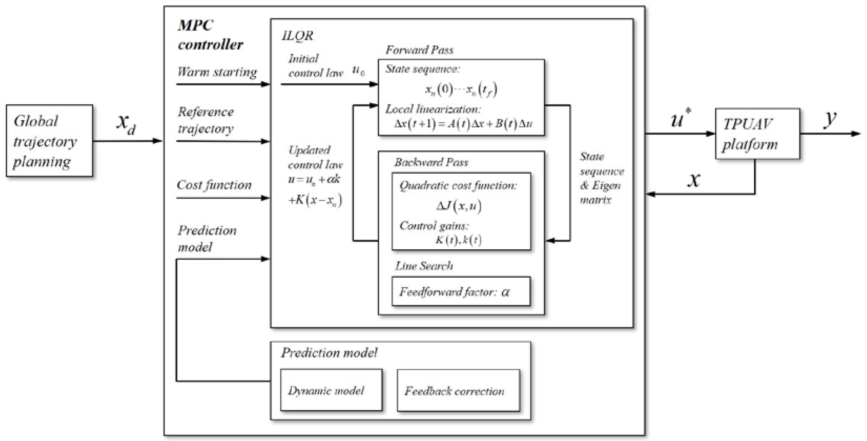
${\mathsf{\Gamma }}_I=\left(x,y,z\right)$ denotes the inertial coordinate frame. ${\mathsf{\Gamma }}_B=\left(x_B,y_B,z_B\right)$ denotes the body coordinate frame attached to the c.g. of TPUAV. ${\mathsf{\Gamma }}_F=\left(x_F,y_F,z_F\right)$ denotes the body translation coordinate frame, and its coordinate origin is fixed on the centre of the front propellers. ${\mathsf{\Gamma }}_D=\left(x_D,y_D,z_D\right)$ denotes the ducted propellers coordinate frame, whose origin is at the center of the ducted propellers.

The external forces of TPUAV are modeled in different coordinate frames, so their action positions and vector directions are different. To concentrate the external forces and moments into the body coordinate frame, a number of transformation matrices are introduced, as follows.

$R_{BI}$ denotes the transformation matrix from the inertial coordinate frame to body coordinate frame, in which simplified expressions are used: $c_{\Theta }=\cos \Theta ,s_{\Theta }=\sin \Theta ,\Theta \in \left\{\varphi ,\theta ,\psi \right\}$.

$$R_{BI}=\left[\begin{array}{ccc}{c}_{\theta }{c}_{\psi }& c_{\theta }{s}_{\psi }& -s_{\theta }\\ s_{\varphi }{s}_{\theta }{c}_{\psi }-c_{\varphi }{c}_{\psi }& s_{\varphi }{s}_{\theta }{s}_{\psi }+c_{\varphi }{c}_{\psi }& s_{\varphi }{c}_{\theta }\\ c_{\varphi }{s}_{\theta }{c}_{\psi }+s_{\varphi }{s}_{\psi }& c_{\varphi }{s}_{\theta }{s}_{\psi }-s_{\varphi }{c}_{\psi }& c_{\varphi }{c}_{\theta }\end{array}\right]$$

(25)

where $\varphi ,\theta ,\psi$ are Euler angles representing roll, pitch, yaw angle, respectively.

$R_{BD}$ denotes the transformation matrix from coordinate ${\mathsf{\Gamma }}_D$ to coordinate ${\mathsf{\Gamma }}_B$.

$$R_{BD}=\left[\begin{array}{ccc}\cos \zeta & 0& \sin \zeta \\ 0& 1& 0\\ -\sin \zeta & 0& \cos \zeta \end{array}\right]$$

(26)

where $\zeta$ represents the tilt angle of the ducted propellers.

The transformation matrix from air coordinate frame to body coordinate frame is $R_{\alpha \beta }$

$$R_{\alpha \beta }=\left[\begin{array}{ccc}\cos \alpha \cos \beta & -\cos \alpha \sin \beta & -\sin \alpha \\ \sin \beta & \cos \beta & -\sin \alpha \sin \beta \\ \sin \alpha \cos \beta & 0& \cos \alpha \end{array}\right]$$

(27)

where $\alpha ,\beta$ represents the angle of attack and angle of sideslip.

The external forces acting on the TPUAV include gravity, aerodynamic force of fuselage, front propellers’ thrust and force produced by ducted propellers. Combining the Equations (2), (3), and (24), the total forces and moments are expressed in the body coordinate frame as follows

$$\left\{\begin{array}{c}{F}_B^{\ast }=R_{\alpha \beta }{F}_{aero}+\left[\begin{array}{c}0\\ 0\\ -T_f\end{array}\right]+R_{BD}\left[\begin{array}{c}{F}_{xd}\\ 0\\ F_{zd}\end{array}\right]+R_{BI}G\\ M_B^{\ast }=R_{\alpha \beta }{M}_{aero}+\left[\begin{array}{c}\left(T_{fl}-T_{fr}\right)b_f/2\\ T_f{c}_f\\ Q_f\end{array}\right]+\left[\begin{array}{c}0\\ M_d-T_d\sin \zeta c_d\\ 0\end{array}\right]\end{array}\right.$$

(28)

where $b_f$ denotes the distance between the left and right hubs of the front propellers, $c_f$ denotes the distance between the midpoint of hubs connection line and the c.m. of TPUAV, $c_d$ denotes the distance from the thrust center point of the ducted propellers to the c.m. of TPUAV, and $G=\left[\begin{array}{c}0\\ 0\\ m_{B}g\end{array}\right]$.

Furthermore, the nonlinear dynamic model, including the translation model and rotation model, could be formulated as follows

$$\left\{\begin{array}{c}\dot{V}=\raisebox{1ex}{$F_B^{\ast }-{\omega }_B\times V$}\!\left/ \!\raisebox{-1ex}{$m_B$}\right.\\ {\dot{\omega }}_{BI}=\raisebox{1ex}{$M_B^{\ast }-{\omega }_B\times I_B{\omega }_B$}\!\left/ \!\raisebox{-1ex}{$I_B$}\right.\end{array}\right.$$

(29)

where $m_B,I_B=\left[\begin{array}{ccc}{I}_{xx}& -I_{xy}& -I_{xz}\\ -I_{xy}& I_{yy}& -I_{yz}\\ -I_{xz}& -I_{yz}& I_{zz}\end{array}\right]$, respectively, represent the mass and moment of inertia of TPUAV, ${\omega }_B=\left[\begin{array}{c}p\\ q\\ r\end{array}\right]$ represents angular velocity vector, and $V=\left[\begin{array}{c}u\\ v\\ w\end{array}\right]$ represents velocity vector.

3. Method

The transition flight of TPUAV is a nonlinear, time-varying process with an aerodynamic coupling effect and strong uncertainty. In order to realize a safe, stable, even optimal transition flight, the transition trajectory plan and controller design is presented in this section.

3.1. ILQR Formulation

Consider a nonlinear system with discrete-time dynamics, which is expressed by the generic form

$$x_{t+1}=f\left(x_t,u_t\right)$$

(30)

This dynamic model describes the evolution from the last time to next in the state $x_t$, given the control $u_t$.

Based on Equation (30), the discretized optimal control problem (OCP) takes the following form

$$\begin{array}{c}\underset{\underset{\_}{x},\underset{\_}{u}}{\min }J=l_T\left(x_T\right)+{\displaystyle \sum _{t=0}^{T-1}l\left(x_t,u_t\right)}\\ s.t.x_0=f_0\\ \forall t=0\cdots T,x_{t+1}=f\left(x_t,u_t\right)\end{array}$$

(31)

where $\underset{\_}{x},\underset{\_}{u}$ represent state and control trajectories, $T$ represents the number of knots, $t$ represents the discrete time, $f_0$ represents the initial state, $l_T,l$ represent terminal and intermediate cost functions, used to define the tasks the UAV has to perform, and to regularize state and control trajectory.

Differential Dynamic Programming (DDP) is an efficient method featuring a super-linear convergence rate with linear complexity in the horizon length. Unlike the Differential Dynamic Programming accounting for the second-order derivatives of the dynamics, ILQR only linearizes the dynamics using Taylor expansion, which is beneficial when simplifying the computation complexity. Then, Equation (31) would be solved by ILQR. Based on Bellman’s principle [34], the optimal solution would be obtained through ILQR cyclic iteration. The control trajectory is obtained in the backward pass, while the state trajectory is updated in the forward pass until the solution reaches convergence.

ILQR computes the state trajectory according to the initial or updated control law in the forward process. Additionally, the system is linearized and a quadratic approximation of the cost function is computed around the reference trajectory.

$$\begin{array}{l}\Delta J\left(x,u\right)=J\left(x+\Delta x,u+\Delta u\right)-J\left(x,u\right)\\ =\frac{1}{2}\Delta x_T^T{l}_{xx}\Delta x_T+l_x\Delta x_T+{\displaystyle \sum _{t=0}^{T-1}\left(\frac{1}{2}\left[\begin{array}{cc}\Delta x_t^T& \Delta u_t^T\end{array}\right]\left[\begin{array}{cc}{l}_{xx}& l_{xu}\\ l_{ux}& l_{uu}\end{array}\right]\left[\begin{array}{c}\Delta x_t\\ \Delta u_t\end{array}\right]+\left[\begin{array}{cc}{l}_x& l_u\end{array}\right]\left[\begin{array}{c}\Delta x_t\\ \Delta u_t\end{array}\right]\right)}\end{array}$$

(32)

Equation (32) denotes the quadratic approximation of cost function around the reference trajectory, where $l_x,l_u,l_{xx},l_{xu},l_{uu}$ are the gradients and Hessians of the cost function.

The value functions and control gains are computed during the backward pass. As with Tassa [26], the second-order expansion of $Q$ is given by

$$\begin{array}{l}{q}_x=l_x+f_x^T{v}_{t+1}\\ q_u=l_u+f_u^T{v}_{t+1}\\ Q_{xx}=l_{xx}+f_x^T{V}_{t+1}{f}_x\\ Q_{xu}=l_{xu}+f_x^T{V}_{t+1}{f}_u\\ Q_{uu}=l_{uu}+f_u^T{V}_{t+1}{f}_u\end{array}$$

(33)

where $f_x,f_u$ are the first derivation of dynamics about state and control.

Then, the optimal control modification $\Delta u^{\ast }$ for $\Delta x$ could be obtained by minimizing the value of $Q$,

$$\Delta u^{\ast }=k_t+K_t\Delta x$$

(34)

Therefore, the feedforward modification and feedback gain matrix are written as

$$\begin{array}{l}{k}_t=-Q_{uu}^{-1}{q}_u\\ K_t=-Q_{uu}^{-1}{Q}_{ux}\end{array}$$

(35)

Then, plugging updated control law back into the $Q$ function, the expression of $V$ is obtained

$$\begin{array}{l}{v}_t=q_x-K_t^T{Q}_{uu}{k}_t\\ V_t=Q_{xx}-K_t^T{Q}_{uu}{K}_t\end{array}$$

(36)

where the backward pass begins from $V_T=l_{xx},v_T=l_x$.

Additionally, the locally linear control law is evaluated with a forward pass once the backward pass is completed. The control law would be optimized by an approach called lineal search [35].

3.2. Global Trajectory Plan Based on ILQR

The transition window of TPUAV is narrow, with many constraints. In order to achieve a safe, stable and even optimal transition flight, it is necessary to comprehensively consider all variables for global trajectory planning to provide a flight reference for the controller.

The essence of the trajectory planning of TPUAV is to find the optimal flight trajectory between the initial state and the terminal state. In this paper, the trajectory planning for the transition process of TPUAV is formed as an optimal control problem, which is solved based on ILQR. The trajectory planning would be completed offline with the global time domain of the transition process, which is run until cost function convergence, and, finally, the optimal control trajectory and state trajectory are obtained. Algorithm 1 summarizes the global trajectory planning of TPUAV.

We denote the state variables by $x=\left[V,q,\theta ,H\right]$, and the corresponding input actions as $u=\left[{\delta }_f,{\delta }_d,{\delta }_e\right]$. The system dynamics of the UAV are discretized for trajectory planning with a sampling time of $t_s$ and a planning horizon of $N$. Let $x\left(t\right),u\left(t\right)$ denote the state and input, respectively, at time-step $t$, and $t_f$ denotes terminal time. To ensure that the states reach the prescribed set points and delivers unputs that are as small as possible in the transition process, it is necessary to design a suitable cost function. The quadratic approximation of the cost function is calculated in ILQR, and the quadratic function is widely used and easy to adjust. Therefore, referring to the standard Bolza form, the cost function of global trajectory planning is designed as:

$$J=\overline{x}{\left(t_f\right)}^T{P}_1 \overline{x}\left(t_f\right)+{\displaystyle {\int }_{t=0}^{t_f}\overline{x}{\left(t\right)}^T{Q}_1 \overline{x}\left(t\right)}+u{\left(t\right)}^T{R}_1 u\left(t\right)dt$$

(37)

where $\overline{x}$ represents the deviation of a state from a desired one, $u$ represents the input, and $P,Q,R$ are the weight matrices of terminal cost, state cost and input cost, respectively. More details about cost function (37) are shown in

Table 1. Weights for state, input and terminal cost of global trajectory plan.

${\mathit{Q}}_1$					${\mathit{R}}_1$			${\mathit{P}}_1$
$V$	$\alpha$	$q$	$\theta$	$H$	${\delta }_f$	${\delta }_d$	${\delta }_e$	$V_f$	${\alpha }_f$	$q_f$	${\theta }_f$	$H_f$
1	0	0.1	1	10	100	100	10	50	0	5	5	500

.

In addition, formulating the tilt angle of ducted propellers as

$$\zeta =\left\{\begin{array}{l}{\zeta }_0={90}^{\circ }\hspace{1em}\hspace{1em}t=0\\ \dot{\zeta }t\hspace{1em}\hspace{1em} 0 < t<t_f\\ {\zeta }_{t_f}=0^{\circ }\hspace{1em}\hspace{1em}t=t_f\end{array}\right.$$

(38)

Algorithm 1. Global trajectory plan based on ILQR

1: Input

2:  System dynamics: $x\left(t+1\right)=f\left(x\left(t\right),u\left(t\right)\right)$

3:  Cost function: $J=\overline{x}{\left(t_f\right)}^T{P}_1 \overline{x}\left(t_f\right)+{\displaystyle \sum _{t=0}^{T-1}\overline{x}{\left(t\right)}^T{Q}_1 \overline{x}\left(t\right)+u{\left(t\right)}^T{R}_1 u\left(t\right)}$

4:  Tilt law: $\zeta \left(t\right)$

5:  Initial control trajectory or law: $u_0\left(t\right)$

6: Output

7:  Optimal control and state trajectory: ${\underset{\_}{u}}^{\ast },{\underset{\_}{x}}^{\ast }$

8: Repeat

9:   Forward Pass

10:  Simulate the system dynamics (nth iteration) in a forward pass:

11:   $\chi :x_n\left(0\right),u_n\left(0\right),\cdots ,x_n\left(t_f-1\right),u_n\left(t_f-1\right),x_n\left(t_f\right)$

12:  Linearize the system dynamics along the trajectory $\chi$:

13:   $\Delta x\left(t+1\right)=A\left(t\right)\Delta x\left(t\right)+B\left(t\right)\Delta u\left(t\right)$

14:  Quadratic Taylor expansion of cost function along $\chi$:

15:   $\Delta J\left(x,u\right)=J\left(x+\Delta x,u+\Delta u\right)-J\left(x,u\right)$

16:   Backward Pass

17:  Based on Bellman’s principle, recursive computation in a backward pass:

18:   $q_x=l_x+f_x^T{v}_{t+1},q_u=l_u+f_u^T{v}_{t+1}$

19:   $Q_{xx}=l_{xx}+f_x^T{V}_{t+1}{f}_x,Q_{xu}=l_{xu}+f_x^T{V}_{t+1}{f}_u,Q_{uu}=l_{uu}+f_u^T{V}_{t+1}{f}_u$

20:   $k_t=-Q_{uu}^{-1}{q}_u,K_t=-Q_{uu}^{-1}{Q}_{ux}$

21:   $v_x=q_x-K_t^T{Q}_{uu}{k}_t,V_{xx}=Q_{xx}-K_t^T{Q}_{uu}{K}_t$

22:   Line Search

23:   Repeat

24:   Update control law: $u_{n+1}\left(t\right)=u_n\left(t\right)+\alpha k\left(t\right)+K\left(t\right)\left(x_{n+1}\left(t\right)-x_n\left(t\right)\right)$

25:   Update state trajectory: $x_{n+1}\left(0\right),\cdots ,x_{n+1}\left(t_f\right)$

26:   Compute new cost: $J_{new}=l_T\left(x_{n+1}\left(t_f\right)\right)+{\displaystyle \sum _{t=0}^{T-1}l\left(x_{n+1}\left(t\right),u_{n+1}\left(t\right)\right)}$

27:   Update feedforward factor: $\alpha =\alpha /{\alpha }_d,{\alpha }_d=const$

28:  Until found lower cost or maximum number of line search reached

29: Until maximum number of iterations or cost function convergence

3.3. Finite Horizon Optimal Control Based on ILQR-MPC

We designed an MPC controller based on ILQR to realize optimal control in a finite horizon. The main concept is that the new flight state constantly triggers MPC updates, and the ILQR within MPC continuously circulates to compute the control trajectory until convergence. Algorithm 2 summarizes the proposed approach.

Algorithm 2. Finite horizon optimal control based on ILQR-MPC

1: Input

2:  Reference trajectory:

3:  optimal state trajectory $x^{\ast }$(produced by global trajectory planning)

4:  System dynamics: $x\left(t+1\right)=f\left(x\left(t\right),u\left(t\right)\right)$

5:  Cost function: $J=\overline{x}{\left(t_f\right)}^T{P}_2 \overline{x}\left(t_f\right)+{\displaystyle \sum _{t=0}^{T-1}\overline{x}{\left(t\right)}^T{Q}_2 \overline{x}\left(t\right)+u{\left(t\right)}^T{R}_2 u\left(t\right)}$

6:  Tilt law: $\zeta \left(t\right)$

7: Output

8:  Optimal control: $u={\underset{\_}{u}}^{\ast }\left(1\right)$

9: Repeat

10:  Warm starting

11:  Initial control trajectory: ${\underset{\_}{u}}_{ 0}=\left[\begin{array}{cccc}{\underset{\_}{u}}^{\ast }\left(2\right)& \cdots & {\underset{\_}{u}}^{\ast }\left(N\right)& {\underset{\_}{u}}^{\ast }\left(N\right)\end{array}\right]$

12:  Run ILQR (similar to Algorithm 1)

13:  Prediction horizon $N$

14:  Weight matrixes $P_2,Q_2,R_2$

15:  Feedback compensation

16:  Prediction model compensation: $f=f_{dyn}+f_{fbc}$

17: Until terminal time

(1) Reference trajectory

The global trajectory planned in Section 3.2 was taken as the reference trajectory of the MPC controller. The tracking effect for global trajectory is an important performance measure during transition flight. We focused on the track of the airspeed and pitch angle of the global trajectory. As the altitude is expected to be stable in transition flight, the desired altitude was designed to be constant.

(2) Cost function

There is a difference in the design requirements for finite-time optimal control and global trajectory plan, so the weights of their cost functions are different. In order to realize smooth transition and utilize the results of the global trajectory plan, the weight of state-tracking was designed to be bigger in the MPC controller. Additionally, the terminal weight was designed, referring to the Riccati solution of LQR.

(3) Warm starting

ILQR of the MPC controller needs to be provided with an initial control trajectory, which determines the convergence speed of ILQR. When running an MPC at a high frequency, the subsequently produced control trajectories usually do not significantly deviate from each other. Therefore, the last controller could provide a good initialization for the next one.

(4) Feedback correction

On the one hand, at each new sampling time, the rolling optimization of MPC controller is realized based on the current state to prevent the system error from being too large to effectively track the desired state because of a model mismatch or external disturbance. On the other hand, according to the error between the system state of TPUAV and the state computed by prediction model, a feedback correction matrix was designed for the uncertainty compensation to correct the system model.

The ILQR-MPC controller continuously updates the control action with its rolling optimization at each sampling time, with stronger robustness and greater control effect than the ILQR controller.

The Control frame is shown in Figure 5.

4. Results

To verify the performance of the ILQR-MPC controller, the simulation results of TPUAV are provided in this section.

4.1. Simulation System Description

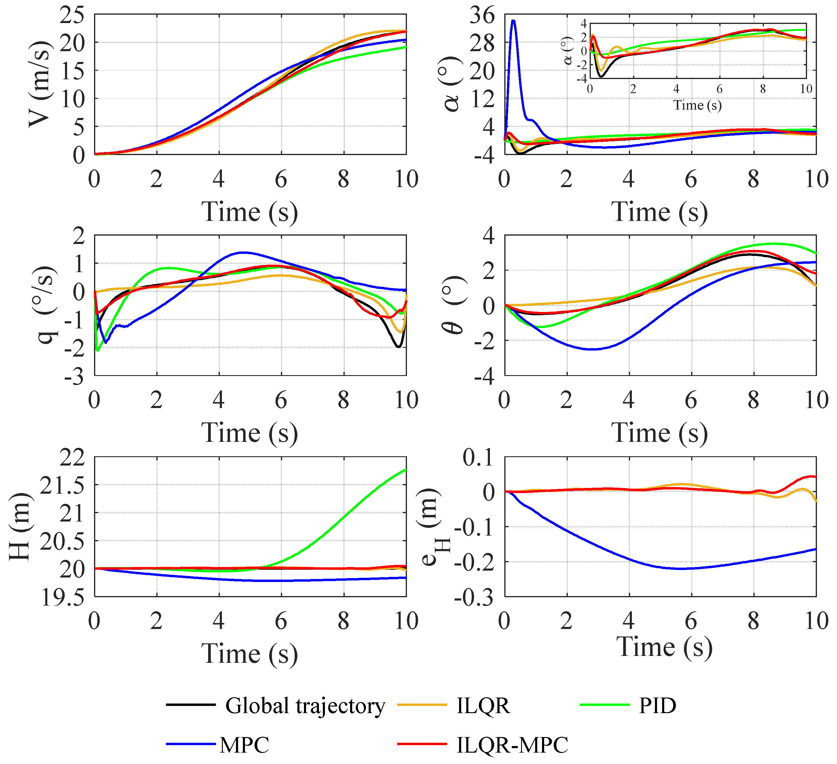
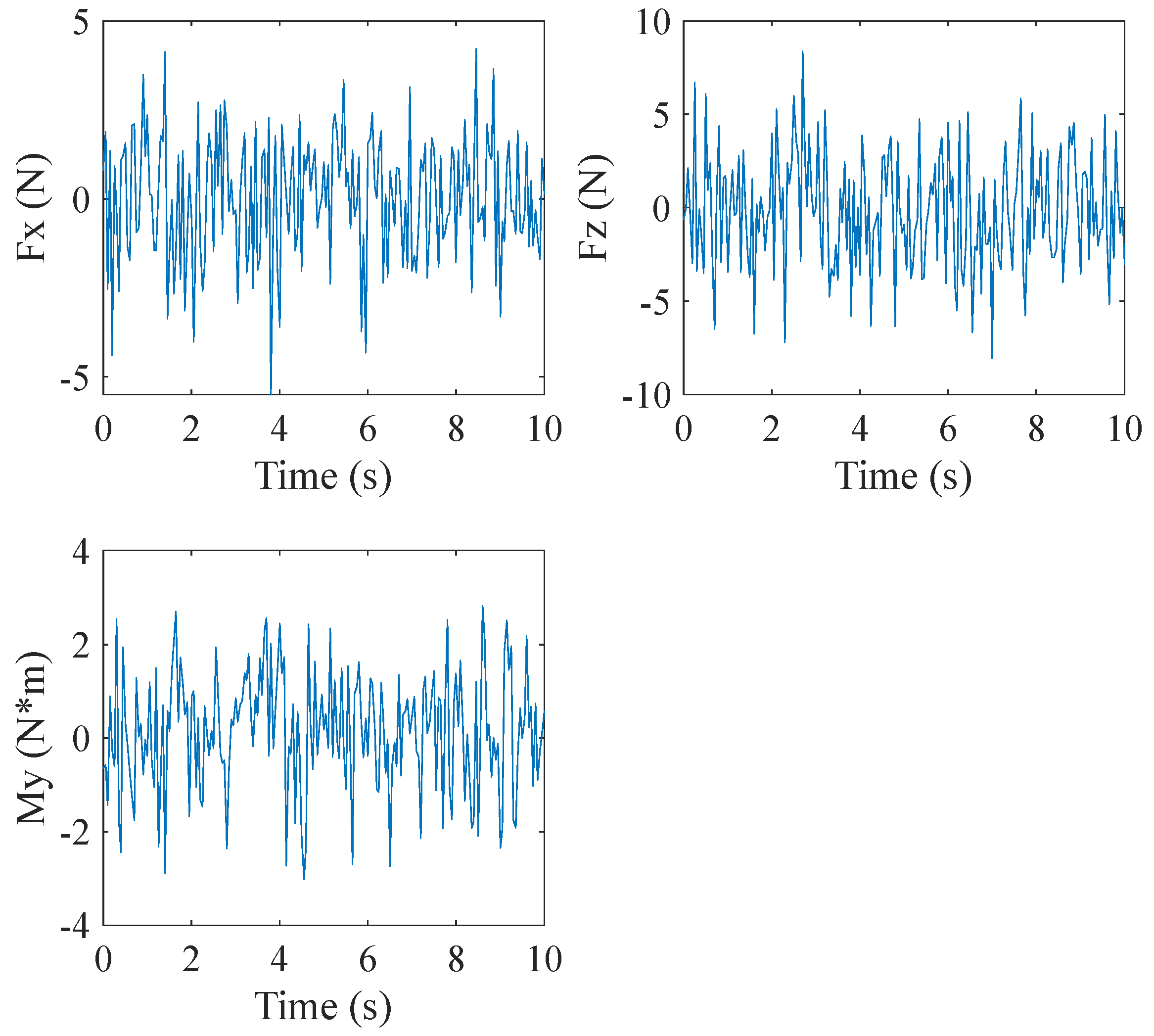
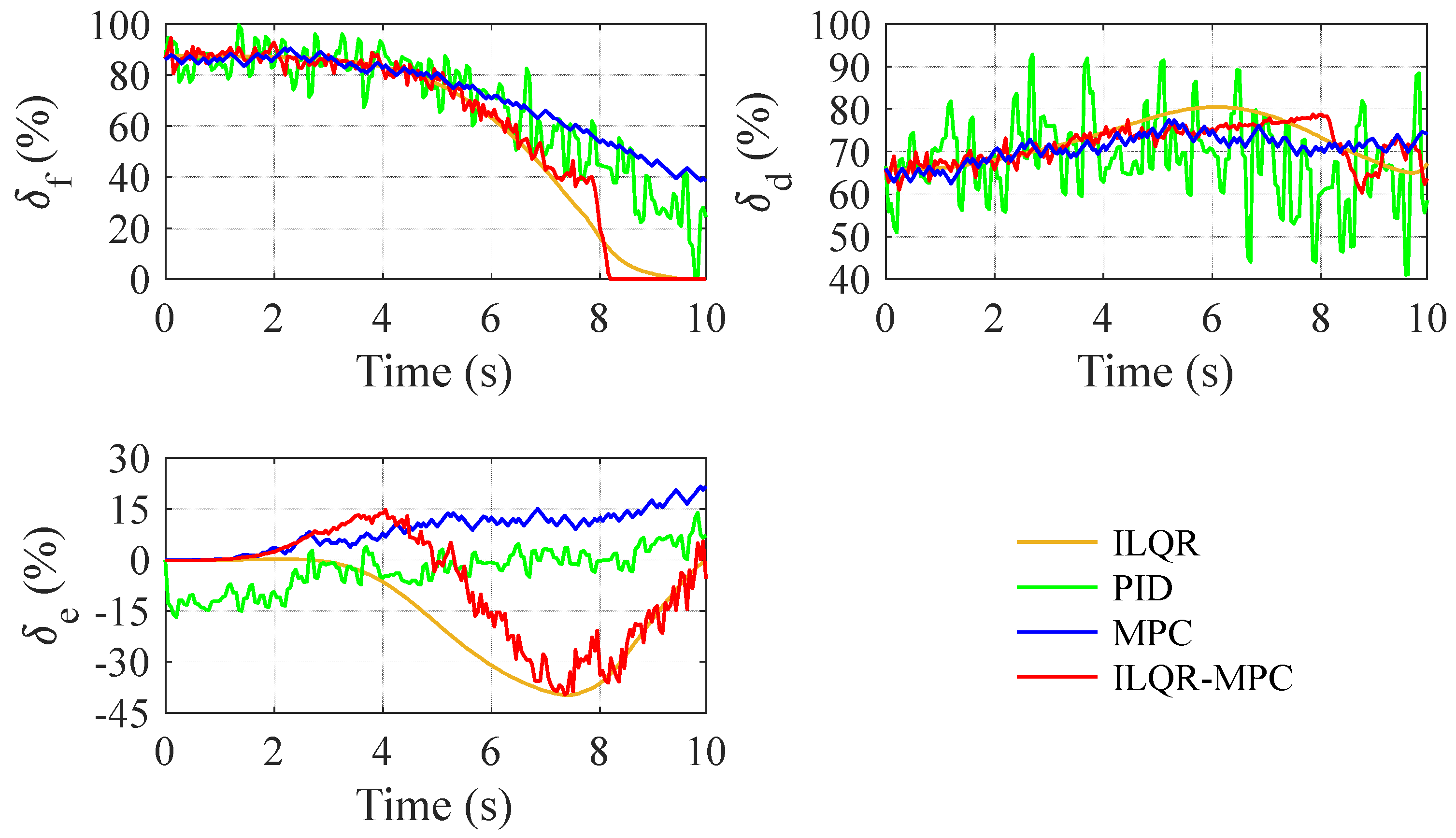
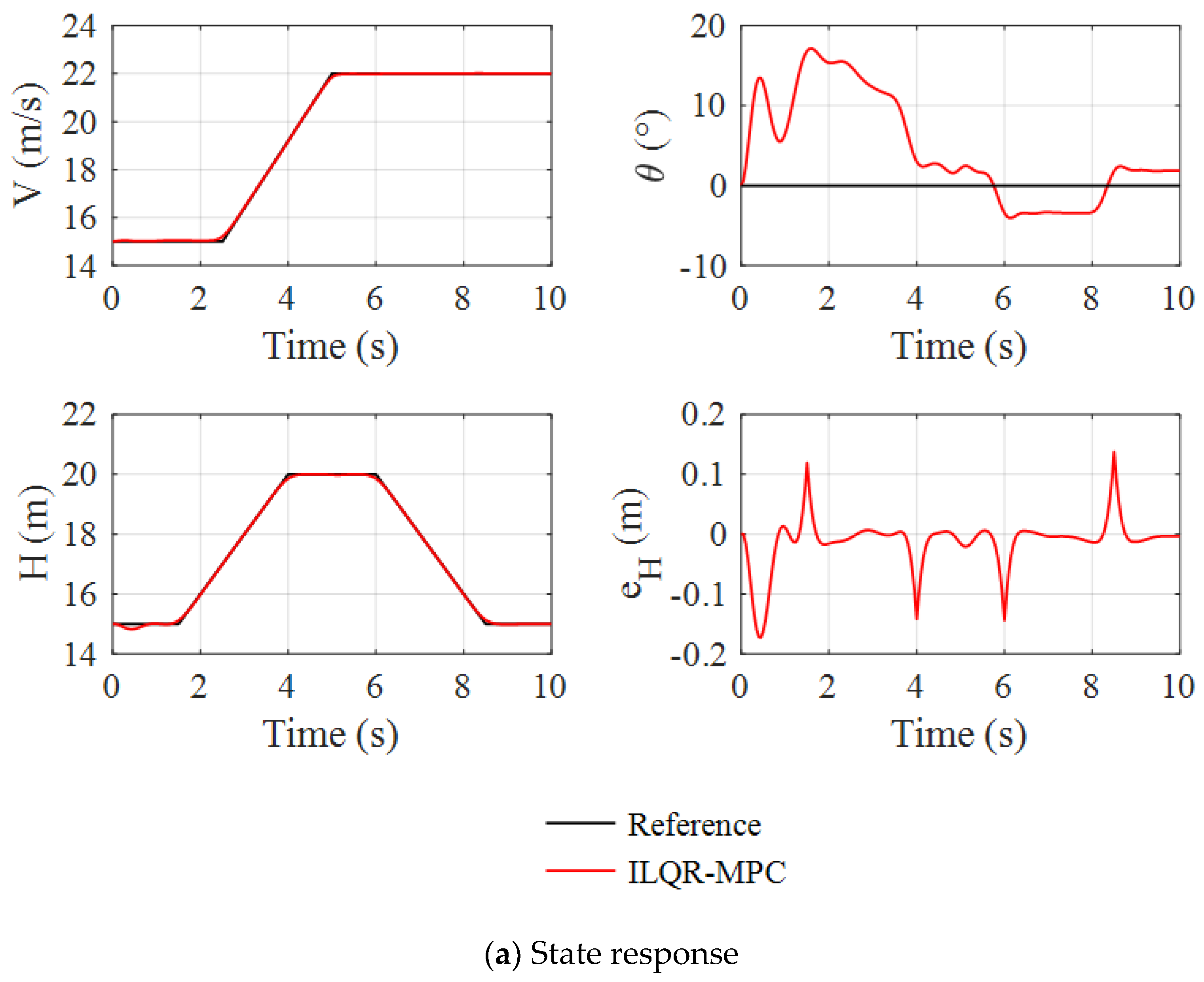
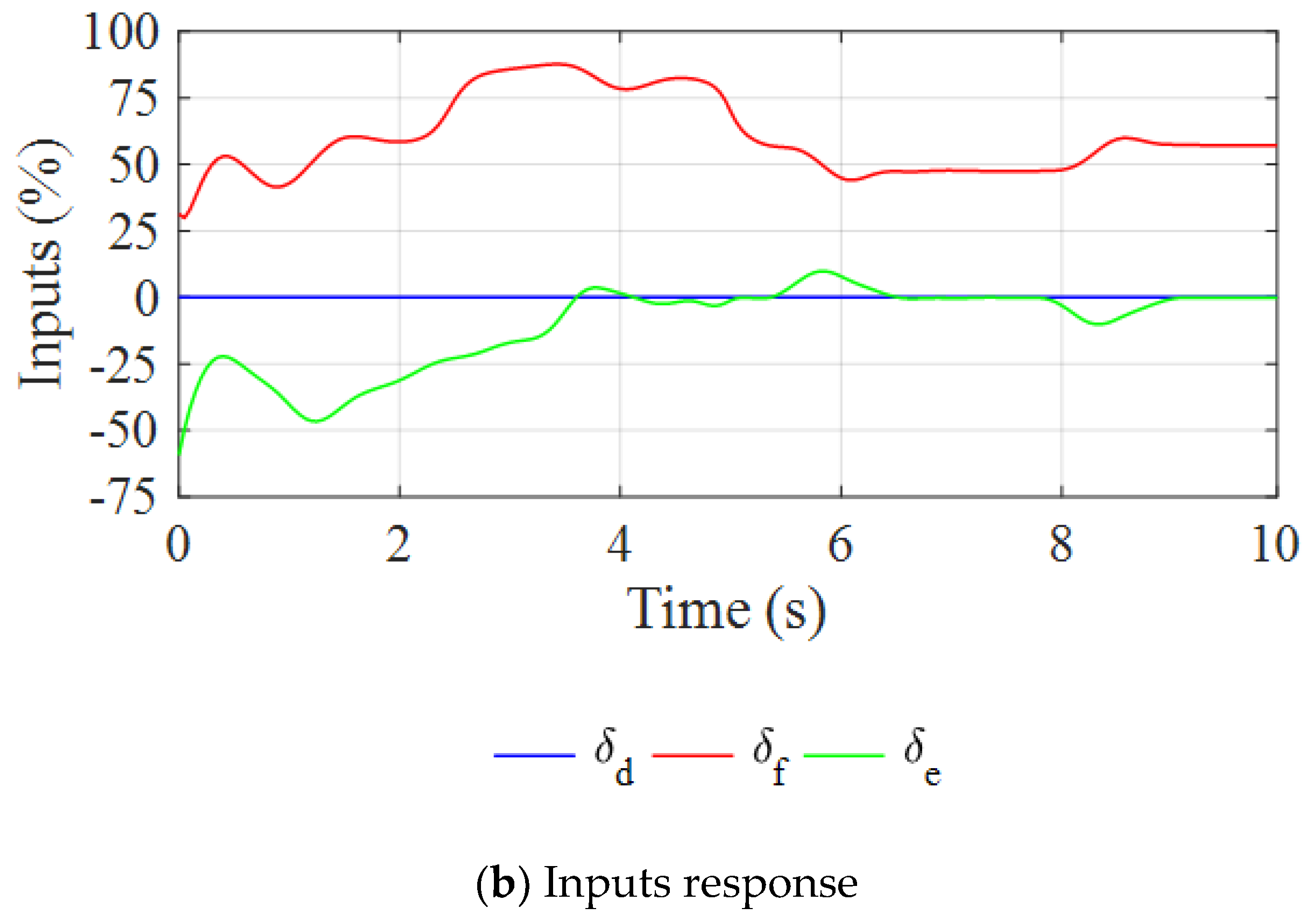
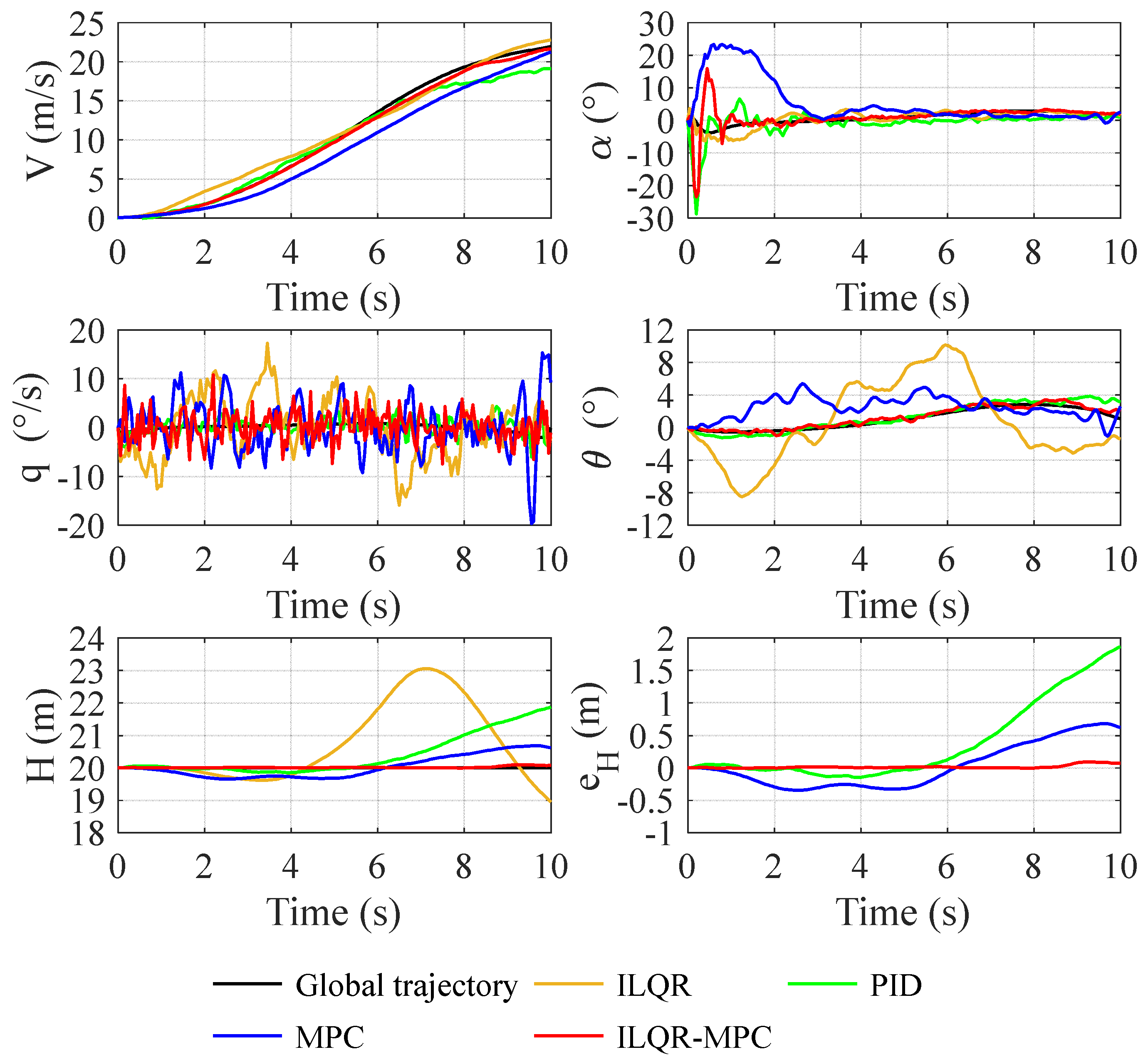
The simulations were carried out based on matlab/simulink with the help of Intel Core i7-1065g7 CPU with 16 GB of RAM.

The model parameters of TPUAV are provided as follows: the mass of UAV is $m=10$kg, the fuselage/wing area is $S=1.01 {\mathrm{m}}^2$, the chord is $c=0.4 \mathrm{m}$, the diameter of front propeller is $R_f=0.28 \mathrm{m}$, the distance from center of front propellers to c.g. is $l_f=0.455 \mathrm{m}$, the diameter of ducted propeller is $R_d=0.14 \mathrm{m}$, and the distance from center of ducted propellers to c.g. is $l_d=0.425 \mathrm{m}$.

4.2. Main Results

A gain scheduling PID controller was designed with reference to commercial autopilot PX4, composed of a rotor controller and a fixed-wing controller. Additionally, an MPC controller was designed simiarly to that of Manzoor et al. [21].

Then, the simulations of transition flight were performed for comparison between the ILQR-MPC with an ILQR feedforward controller, the PID controller and the MPC controller.

Before control performance verification, we planned the global trajectory for the transition flight first. Compared with the tracking terminal desired state, the tracking global trajectory would gain a smoother state variation and avoid input saturation.

The simulations would be performed based on conditions without and with uncertainty, respectively, as in the following. The initial states of TPUAV are denoted as follows:

$$V_0=0.1 \mathrm{m}/\mathrm{s},{\alpha }_0=0^{\circ },q_0=0^{\circ }/\mathrm{s},{\theta }_0=0^{\circ },H_0=20 \mathrm{m},{\zeta }_0={90}^{\circ }$$

(39)

The prediction horizon, control horizon and sample time employed in this paper are given as $N_c=N_p=40$, $ts=0.05 \mathrm{s}$.

The cost function (shown in Algorithm 2) of the MPC controller is designed as MPC

$$J=\overline{x}{\left(t_f\right)}^T{P}_2 \overline{x}\left(t_f\right)+{\displaystyle \sum _{t=0}^{T-1}\overline{x}{\left(t\right)}^T{Q}_2 \overline{x}\left(t\right)+u{\left(t\right)}^T{R}_2 u\left(t\right)}$$

(40)

The design of the cost function of the MPC controller is based on multiple optimization objectives, among which good tracking for the reference trajectory is the most important one. In addition, the input should be as small as possible to save energy consumption in the transition flight.

To improve the performance of the controller, the weights were empirically tuned during the testing process (shown in

Table 2. Weights for state, input and terminal cost of MPC controller.

${\mathit{Q}}_2$					${\mathit{R}}_2$			${\mathit{P}}_2$
$V$	$\alpha$	$q$	$\theta$	$H$	${\delta }_f$	${\delta }_d$	${\delta }_e$	$V_f$	${\alpha }_f$	$q_f$	${\theta }_f$	$H_f$
1	0	0.1	1	10	20	20	2	5	0	0.5	0.5	50

).

Under the condition of no uncertainty (shown in Figure 6 and Figure 7), both the ILQR feedforward controller and ILQR-MPC controller achieve an excellent control effect. Both controllers have smooth inputs, maintain the altitude at the desired point, and realize the airspeed and pitch angle well-tracking. However, the PID controller based on the PX4 framework has a general control effect from the tracking of airspeed and pitch angle, and has obvious deviations in the most important altitude tracking. Due to the single-input and single-output characteristics, PID controller cannot account for altitude, speed and pitch angle tracking at the same time. Even the altitude sub-controller and attitude sub-controller compete for the control ability, so cooperative control between multiple inputs and multiple outputs cannot be realized. The computation of MPC depends on the linearization dynamics at the initial time of the finite horizon. Unfortunately, the transition flight is a complex, nonlinear, time-varying process, so the model error in MPC is more significant than that of ILQR-MPC, which linearizes the dynamics along the trajectory. Therefore, the control effect of MPC controller is slightly inferior to that of the ILQR-MPC controller. However, it has better control precision than the PID controller.

The manipulation difference between ILQR-MPC and PID controllers is mainly shown in the second half of the transition flight (5 s~10 s). The throttle of the ducted propellers ${\delta }_d$ of the ILQR-MPC controller is significantly higher than that of the PID controller, while the throttle of the front propeller ${\delta }_f$ of the ILQR-MPC controller is lower. In addition, the ${\delta }_e$ is smaller, meaning that the upward deflection angle of elevon is larger based on the ILQR-MPC controller (the downward deflection is positive). When the tilt angle of the ducted propellers is large, the UAV overcomes the drag by lowering its head, while the UAV relies on the thrust horizontal component of the ducted propellers to obtain a stronger acceleration ability when the tilt angle is small. The ${\delta }_d$ of the ILQR-MPC controller is larger, so it achieves better speed-tracking in transition flight. After 8s, ${\delta }_f$ of the ILQR-MPC controller reduces to zero; that is, the front propellers stop, which is a reasonable operation for the following two reasons: on the one hand, a smaller ${\delta }_f$ leads to more energy being saved, and on the other hand, as the flight mode gradually changes to a fixed-wing mode, the front-propeller propellers are no longer required to provide lift. In second half of the transition flight, the airspeed is big enough, and the attitude control has a better efficiency based on aerodynamic surfaces than the thrust differential produced by the front propellers and the ducted propellers, so the elevation deflection angle of the ILQR-MPC controller is larger.

Considering that there are uncertainties such as system modeling errors and external environment disturbance, more simulations are taken for conditions with uncertainty in transition flight. System uncertainties in simulations are modeled as the Gaussian white noise (shown in Figure 8), with different noise intensities in each direction according to their characteristics.

Figure 9 and Figure 10 respectively show the State and inputs responses during transition flight with uncertainty.

The ILQR feedforward controller cannot suppress the significant uncertainty leading to the rapid deterioration in the control effects, which leads to serious altitude errors, and even the risk of crash. Although the control effect of the PID controller is only slightly reduced, the inputs are greatly shaken, bringing a great burden to actuators.

Based on feedback correction, MPC and ILQR-MPC have the advantage of disturbance rejection. Therefore, the altitude tracking error of the ILQR-MPC controller is very small during the whole transition flight, with the smooth change in airspeed and pitch angle. ILQR-MPC linearizes the dynamics along the state trajectory, which has two advantages. On the one hand, the ILQR-MPC has linear complexity to improve the computation efficiency and greatly reduces the difficulty in solving nonlinear problems. On the other hand, the method with dynamics linearization at discrete points has a higher control precision than MPC [21]. To suppress the disturbance caused by high-frequency Gaussian white noise, the input variation in MPC and ILQR-MPC controllers is no longer smooth. However, based on the receding horizontal optimization, MPC and ILQR-MPC controllers can make full use of the dynamics used to predict states in the future time domain; therefore, the chattering of inputs is much smaller than that of the PID controller. Overall, compared with the ILQR feedforward controller, PID controller and MPC controller, ILQR-MPC can deal with uncertainties more effectively, with stable inputs and state tracking.

4.3. Implementation

The ILQR-MPC controller proposed in this paper is suitable for a full flight envelope. Although the main goal is to achieve the optimal transition flight of TPUAV, the controller is also applicable to rotor and fixed-wing modes. In order to prove the full envelope control ability of the ILQR-MPC controller, two simulations would be designed, in the rotor mode and fixed-wing mode, respectively.

Under the rotor mode, the tilt angle of the ducted propeller is ${90}^{\circ }$, and the core indexes are altitude-tracking and velocity-tracking. The reference trajectory is designed as $H_c=20 \mathrm{m},V_c=\left\{\begin{array}{l}8 \mathrm{m}/\mathrm{s}\hspace{1em}2 \mathrm{s}\le t\le 6 \mathrm{s}\\ 5 \mathrm{m}/\mathrm{s}\hspace{1em}else\end{array}\right.,{\theta }_c=0^{\circ }$.

The results in Figure 11 show that the ILQR-MPC controller has a fast and accurate tracking response with a smooth change of states. TPUAV lowers its head quickly to improve velocity near the time of $2 \mathrm{s}$, and raises its head sharply near the time of $6 \mathrm{s}$ to realize rapid deceleration by the horizontal component of thrust and aerodynamic resistance. Under this velocity step commander, the altitude tracking error is kept within $0.2 \mathrm{m}$, which reflects the applicability of the ILQR-MPC controller in the rotor mode.

Subsequently, the reference trajectory for fixed-wing mode simulation is designed as

$$\begin{array}{l}{H}_c=\left\{\begin{array}{l}\begin{array}{c} 15 \mathrm{m}\hspace{1em}\hspace{1em}\hspace{1em}\hspace{1em}\hspace{1em}\hspace{1em}\mathrm{t}\le 1.5 \mathrm{s}\\ 15+2(\mathrm{t}-1.5) \mathrm{m}\hspace{1em}1.5 \mathrm{s}<\mathrm{t}\le 4 \mathrm{s}\\ 20 \mathrm{m}\hspace{1em}\hspace{1em}\hspace{1em}\hspace{1em}\hspace{1em}\hspace{1em}4 \mathrm{s}<\mathrm{t}\le 6 \mathrm{s}\end{array}\\ \begin{array}{c}\hspace{1em}20-2(\mathrm{t}-1.5) \mathrm{m}\hspace{1em}6 \mathrm{s}<\mathrm{t}\le 8.5 \mathrm{s}\\ 15 \mathrm{m}\hspace{1em}\hspace{1em}\hspace{1em}\hspace{1em}\hspace{1em}\hspace{1em}\mathrm{t}>8.5 \mathrm{s}\end{array}\end{array}\right., \\ V_c=\left\{\begin{array}{c}15 \mathrm{m}/\mathrm{s}\hspace{1em}\hspace{1em}\hspace{1em}\hspace{1em}\hspace{1em}\hspace{1em}\mathrm{t}\le 2.5 \mathrm{s}\\ 15+2.8\left(\mathrm{t}-2.5\right) \mathrm{m}/\mathrm{s}\hspace{1em}2.5 \mathrm{s}<\mathrm{t}\le 5 \mathrm{s}\\ 22 \mathrm{m}/\mathrm{s}\hspace{1em}\hspace{1em}\hspace{1em}\hspace{1em}\hspace{1em}\hspace{1em}\mathrm{t}>5 \mathrm{s}\end{array}\right.,{\theta }_c=0^{\circ }\end{array}$$

Under fixed-wing mode, the tilt angle of ducted propeller is $0^{\circ }$, and the altitude tracking and velocity tracking are still core indexes.

In this simulation shown as Figure 12, TPUAV accelerates to cruise speed and goes through the process of first climbing and then descending. The throttle input of the ducted propeller is large during the acceleration process, while the throttle input remains stable in final cruise flight. When TPUAV climbs, the path angle is positive, so the pitch angle is large. On the contrary, when TPUAV descends, the path angle is negative, and the pitch angle is small. Under the complex flight command, the altitude tracking error remains within $0.2 \mathrm{m}$, which reflects the applicability of the ILQR-MPC controller in fixed-wing mode.

In addition, the $R$ matrix of the controller in rotor and fixed-wing modes are different from the transition flight, which are proposed as $R_{rotor}=diag\left(20,20,2000\right)$, $R_{rotor}=diag\left(2000,20,20\right)$ for a simpler and clearer control logic.

5. Conclusions

This work presents a new MPC controller for the transition flight of tilt-propulsion UAV, and verifies the controller performance using simulations. To accurately describe the dynamic behavior of UAV in transition flight, a ducted propeller model with aerodynamic/propulsion coupling is proposed; furthermore, a high-precision dynamic model is developed. Then, a control framework of transitional flight, including offline global trajectory planning and online finite-horizon control is proposed, which has good computation efficiency to solve nonlinear problems such as transition flights due to the application of ILQR. The finite-horizon controller is a unified MPC controller for the full transition envelope, which could be applied from the rotor mode to fixed-wing mode, making full use of configurations to develop the control potential of UAV. The simulations show that the ILQR-MPC controller has a better control effect, more reasonable control logic, and stronger anti-interference ability compared with the ILQR feedforward controller, gain scheduling PID controller and MPC controller.

References

1. Zhang, T.; Barakos, G.N. Toward Vehicle-Level Optimization of Compound Rotorcraft Aerodynamics. AIAA J. 2021, 60, 1937–1957. [Google Scholar] [CrossRef]
2. Xia, J.Y.; Zhou, Z.; Xu, D.; Wang, Z. Aerodynamic/Propulsion Coupling Model of Vector Electric Propulsion System. Acta Aeronaut. Astronaut. Sin. 2022, 25, 1–12. Available online: http://kns.cnki.net/kcms/detail/11.1929.V.20220829.1342.002.html (accessed on 1 September 2022).
3. Ducard, G.J.; Allenspach, M. Review of designs and flight control techniques of hybrid and convertible VTOL UAVs. Aerosp. Sci. Technol. 2021, 118, 107035. [Google Scholar]
4. Yang, Y.J.; Zhu, J.H.; Wang, X.Y.; Yuan, X.; Zhang, X. Dynamic Transition Corridors and Control Strategy of a Rotor-Blown-Wing Tail-Sitter. J. Guid. Control. Dyn. 2021, 44, 1836–1852. [Google Scholar] [CrossRef]
5. Cardoso, D.N.; Esteban, S.; Raffo, G.V. A new robust adaptive mixing control for trajectory tracking with improved forward flight of a tilt-rotor UAV. ISA Trans. 2021, 110, 86–104. [Google Scholar] [CrossRef] [PubMed]
6. Liu, N.J.; Cai, Z.H.; Wang, Y.X.; Zhao, J. Fast level-flight to hover mode transition and altitude control in tilt-rotor’s landing operation. Chin. J. Aeronaut. 2021, 34, 181–193. [Google Scholar] [CrossRef]
7. Hartmann, P.; Meyer, C.; Moormann, D. Unified Velocity Control and Flight State Transition of Unmanned Tilt-Wing Aircraft. J. Guid. Control. Dyn. 2017, 40, 1348–1359. [Google Scholar] [CrossRef]
8. Li, B.Y.; Sun, J.X.; Zhou, W.F.; Wen, C.-Y.; Low, K.H.; Chen, C.-K. Transition Optimization for a VTOL Tail-sitter UAV. IEEE/ASME Trans. Mechatron. 2020, 25, 2535–2545. [Google Scholar] [CrossRef]
9. Liu, H.; Peng, F.C.; Lewis, F.L.; Wan, Y. Robust Tracking Control for Tail-Sitters in Flight Mode Transitions. IEEE Trans. Aerosp. Electron. Syst. 2019, 55, 2023–2035. [Google Scholar] [CrossRef]
10. Cakici, F.; Leblebicioglu, M.K. Control System Design of a Vertical Take-off and Landing Fixed Wing UAV. IFAC-Pap. Online 2016, 49, 267–272. [Google Scholar] [CrossRef]
11. Wang, Z.G.; Zhao, H.; Duan, D.; Jiao, Y.; Li, J. Application of improved active disturbance rejection control algorithm in tilt quad rotor. Chin. J. Aeronaut. 2020, 33, 1625–1641. [Google Scholar] [CrossRef]
12. Quan, Q.; Fu, R.; Li, M.X. Practical Distributed Control for VTOL UAVs to Pass a Virtual Tube. IEEE Trans. Intell. Veh. 2022, 7, 342–353. [Google Scholar] [CrossRef]
13. Liu, Z.; Theilliol, D.; Yang, L.; He, Y.; Han, J. Observer-based linear parameter varying control design with unmeasurable varying parameters under sensor faults for quad-tilt rotor unmanned aerial vehicle. Aerosp. Sci. Technol. 2019, 92, 696–713. [Google Scholar] [CrossRef]
14. Mayne, D.Q.; Rawlings, J.B.; Rao, C.V.; Scokaert, P.O.M. Constrained model predictive control: Stability and optimality. Automatica 2000, 36, 789–814. [Google Scholar] [CrossRef]
15. Papachristos, C.; Alexis, K.; Tzes, A. Hybrid model predictive flight mode conversion control of unmanned quad-tiltrotors. In Proceedings of the IEEE European Control Conference (ECC), Zurich, Switzerland, 17–19 July 2013. [Google Scholar]
16. Vukov, M.; Domahidi, A.; Ferreau, H.J.; Morari, M.; Diehl, M. Auto-generated Algorithms for Nonlinear Model Predicative Control on Long and on Short Horizons. In Proceedings of the 52nd IEEE Conference on Decision and Control, Firenze, Italy, 10–13 December 2013. [Google Scholar]
17. Quirynen, R.; Vukov, M.; Zanon, M.; Diehl, M. Autogenerating Microsecond Solvers for Nonlinear MPC: A Tutorial Using ACADO Integrators. Optim. Control. Appl. Methods 2015, 36, 685–704. [Google Scholar] [CrossRef]
18. Kamel, M.; Alexis, K.; Achtelik, M.; Siegwart, R. Fast nonlinear model predictive control for multicopper attitude tracking on SO(3). In Proceedings of the IEEE Multi-Conference on Systems and Control, Sydney, NSW, Australia, 21–23 September 2015. [Google Scholar]
19. Papachristos, C.; Alexis, K.; Tzes, A. Dual-Authority Thrust-Vectoring of a Tri-TiltRotor employing Model Predictive Control. J. Intell. Robot. Syst. 2016, 81, 417–505. [Google Scholar] [CrossRef]
20. Allenspach, M.; Ducard, G.J. Model predictive control of a convertible tiltrotor unmanned aerial vehicle. In Proceedings of the 28th Mediterranean Conference on Control and Automation (MED), Saint-Raphael, France, 15–18 September 2020. [Google Scholar]
21. Manzoor, T.; Xia, Y.Q.; Zhai, D.-H.; Ma, D. Trajectory tracking control of a VTOL unmanned aerial vehicle using offset-free tracking MPC. Chin. J. Aeronaut. 2020, 33, 2024–2042. [Google Scholar] [CrossRef]
22. Bauersfeld, L.; Spannagl, L.; Ducard, G.J.J.; Onder, C.H. MPC Flight Control for a Tilt-rotor VTOL Aircraft. IEEE Trans. Aerosp. Electron. Syst. 2021, 57, 2395–2409. [Google Scholar] [CrossRef]
23. Mayne, D.Q. Differential Dynamic Programming—A Unified Approach to the Optimization of Dynamic Systems. Control. Dyn. Syst. 1973, 10, 179–254. [Google Scholar]
24. Budhiraja, R.; Carpentier, J.; Mastalli, C.; Mansard, N. DDP for multi-phase rigid contact dynamics. In Proceedings of the IEEE-RAS 18th International Conference on Humanoid Robots (Humanoids), Beijing, China, 6–9 November 2018. [Google Scholar]
25. Todorov, E.; Li, W.W. A generalized iterative LQG method for locally-optimal feedback control of constrained nonlinear stochastic systems. In Proceedings of the IEEE American Control Conference, Portland, OR, USA, 8–10 June 2005. [Google Scholar]
26. Tassa, Y.; Mansard, N.; Todorov, E. Control-Limited Differential Dynamic Programming. In Proceedings of the IEEE International Conference on Robotics & Automation (ICRA), Hong Kong, China, 29 September 2014. [Google Scholar]
27. Grandia, R.; Farshidian, F.; Ranftl, R.; Hutter, M. Feedback MPC for Torque-Controlled Legged Robots. In Proceedings of the IEEE/RSJ International Conference on Intelligent Robots and Systems (IROS), Macau, China, 3–8 November 2019. [Google Scholar]
28. Dantec, E.; Taïx, M.; Mansard, N. First Order Approximation of Model Predictive Control Solutions for High Frequency Feedback. IEEE Robot. Autom. Lett. 2022, 7, 4448–4455. [Google Scholar] [CrossRef]
29. Werle, M.J. Analytical Model for Ring-Wing Propulsor Thrust Augmentation. J. Aircr. 2020, 57, 901–913. [Google Scholar] [CrossRef]
30. McCormick, B.W. Aerodynamics of V/STOL Flight; Dover Publications: Mineola, NY, USA, 1999. (In English) [Google Scholar]
31. Werle, M.J. Analytical Model for Ring-Wing Propulsors at Angle of Attack. J. Aircr. 2022, 59, 1–12. [Google Scholar] [CrossRef]
32. Lewis, R.I. Vortex Element Methods for Fluid Dynamic Analysis of Engineering Systems; Cambridge University Press: Cambridge, UK, 1991; pp. 191–227. [Google Scholar]
33. Werle, M.J. Aerodynamic Loads and Moments on Axisymmetric Ring-Wing Ducts. AIAA J. 2014, 52, 2359–2361. [Google Scholar] [CrossRef]
34. Bellman, R.R. Dynamic programming. Science 1966, 153, 34–37. [Google Scholar] [CrossRef] [PubMed]
35. Neunert, M.; de Crousaz, C.; Furrer, F.; Kamel, M.; Farshidian, F.; Siegwart, R.; Buchli, J. Fast Nonlinear Model Predictive Control for Unified Trajectory Optimization and Tracking. In Proceedings of the IEEE International Conference on Robotics and Automation (ICRA), Stockholm, Sweden, 9 June 2016. [Google Scholar]
Figure 1. Tilt-propulsion UAV configuration.
Aerospace 09 00688 g001
Figure 2. Typical stations of ducted propeller.
Aerospace 09 00688 g002
Figure 3. Ducted propellers in experiment.
Aerospace 09 00688 g003
Figure 4. Parameters of ducted propellers.
Aerospace 09 00688 g004
Figure 5. Control frame.
Aerospace 09 00688 g005
Figure 6. State response during transition flight without uncertainty.
Aerospace 09 00688 g006
Figure 7. Input response during transition flight without uncertainty.
Aerospace 09 00688 g007
Figure 8. Gaussian noises.
Aerospace 09 00688 g008
Figure 9. State response during transition flight with uncertainty.
Aerospace 09 00688 g009
Figure 10. Inputs response during transition flight with uncertainty.
Aerospace 09 00688 g010
Figure 11. State and inputs response in rotor mode.
Aerospace 09 00688 g011
Figure 12. State and inputs response in fixed-wing mode.
Aerospace 09 00688 g012aAerospace 09 00688 g012b