Longitudinal Aerodynamic Parameter Identification for Blended-Wing-Body Aircraft Based on a Wind Tunnel Virtual Flight Test

Abstract

The wind tunnel virtual flight test realizes the dynamic semi-free flight of the model in the wind tunnel through the deflections of the control surface and uses the test data to identify the aerodynamic derivatives. The difference in dynamics between the wind tunnel virtual flight and the free flight leads to discrepancies between the identification and theoretical results. To solve the problems, a step-by-step identification and correction method for aerodynamic derivatives is established based on the difference between the equations of motion of wind tunnel virtual flight and free flight to identify and correct the lift, drag derivatives, pitch moment derivatives, and velocity derivatives, respectively. To establish an aerodynamic parameter identification model, the flight dynamics equation is expressed as a decoupled form of the free flight force and the influence of the test support frame force on the model’s motions through linearization. To ensure the identification accuracy of each aerodynamic derivative, an excitation signal design method based on amplitude–frequency characteristic analysis is proposed. The longitudinal aerodynamic parameter identification results of a blended-wing-body aircraft show that identification results with higher accuracy can be obtained by adopting the proposed identification and correction method.

1. Introduction

The traditional wind tunnel test and aerodynamic modeling technology are based on the linear superposition principle [1]. Static wind tunnel tests are used to obtain constant aerodynamic data and forced oscillation tests are used to obtain dynamic derivative data, so that the aerodynamic model of the aircraft can be finally constructed [2]. However, traditional force measurements are occasionally inaccurate. Aerodynamic parameter identification is based on the aircraft’s control surface input and flight response data to identify the aerodynamic derivatives, which are then compared and corrected with wind tunnel force measurements [3].

At present, the actual flight of a real aircraft is generally used for the identification of aerodynamic parameters, and the results obtained by this method are highly accurate, but there are many problems, such as high cost and high risk [4,5,6], and the actual flight is usually carried out in the late design cycle. In the early stage of aircraft design, a scaled model of the aircraft is installed in a wind tunnel for dynamic flight to approximate real flight, and then the test data are used to identify the aerodynamic parameters compared with traditional wind tunnel force measurement data. This new test technique is called wind tunnel virtual flight tests [7]. 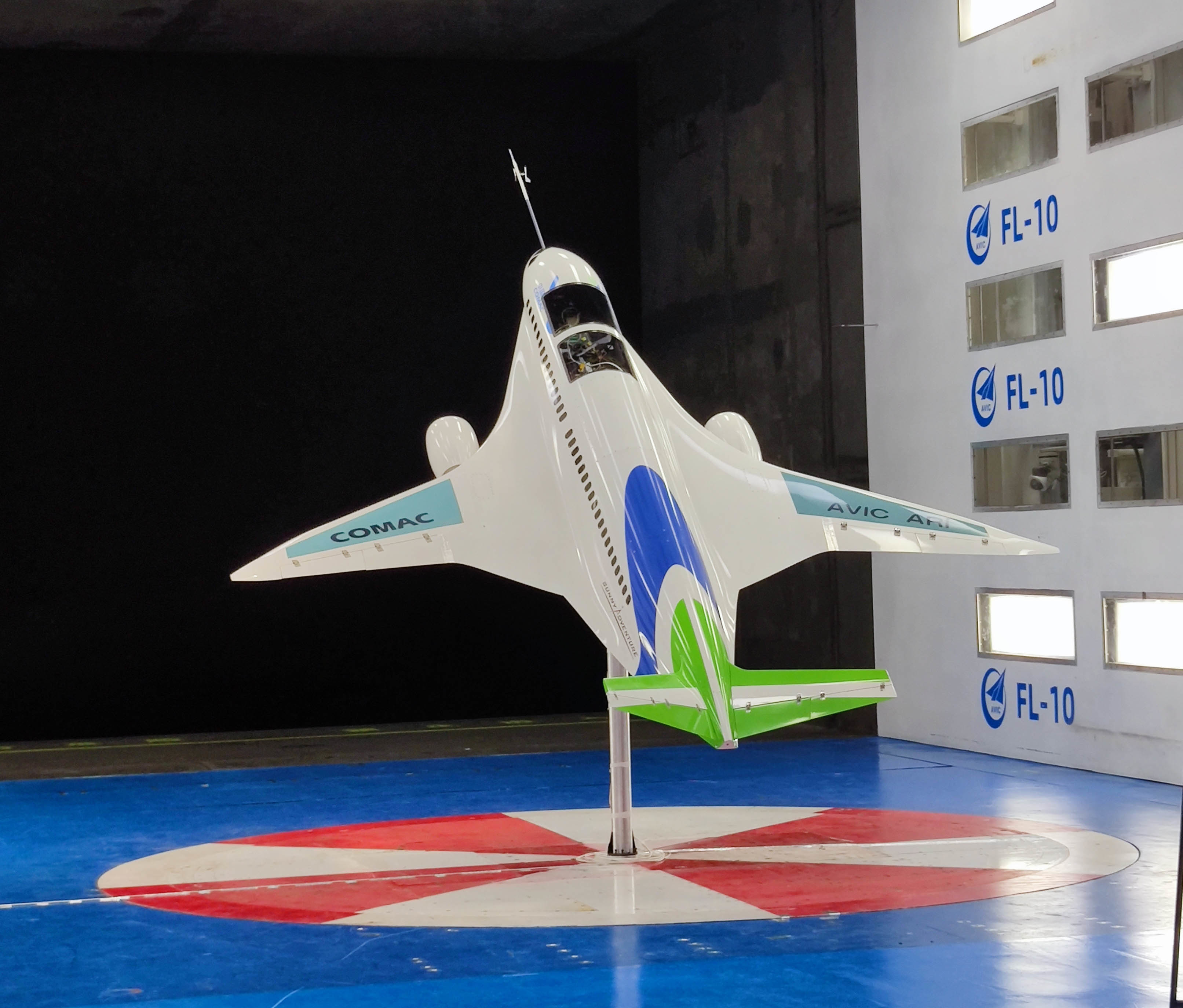As shown in Figure 1, the most widely used wind tunnel virtual flight test generally refers to a 3-DOF dynamic wind tunnel test. The model aircraft is connected to the strut through a 3-DOF rotation mechanism and installed in the wind tunnel test section so that the model displacement is constrained but has 3 degrees of angular motion freedom. Open-loop and closed-loop control of the aircraft model is achieved by directly driving the control surface or by using commands from the flight control system. Many scholars also refer to this wind tunnel virtual flight test setup as the “multi-degree-of-freedom test rig” [5]. In traditional wind tunnel tests, the aircraft cannot move autonomously, but in the wind tunnel virtual flight test, the motion of the model is realized by manipulating the surface deflections.

The blended-wing-body (BWB) aircraft studied in this article refers to a new layout aircraft that eliminates the tail and uses a V-tail instead of horizontal and vertical tails [8,9], as shown in Figure 1. This layout has a shorter fuselage size, less longitudinal stability, and less pitch damping [10]. If the aerodynamic derivatives within the full envelope of the model are identified by wind tunnel virtual flight tests, the attitude angle of the model needs to be precisely controlled so that it varies within the desired range. Open-loop control cannot accurately control the attitude of the model in the wind tunnel test [11], and the model may deviate from the original equilibrium state point after the excitation signal input. Therefore, it is necessary to design control augmentation laws for the BWB test model, carry out control surface excitation for the closed-loop controlled model, and complete the study of aerodynamic parameter identification for the wind tunnel virtual flight test. There are still some new problems that need to be solved for the identification of longitudinal aerodynamic parameters of BWB aircraft under closed-loop control for a wind tunnel virtual flight test.

Due to the displacement constraints that lead to the difference between the equations of motion for wind tunnel virtual flight and free flight, the motions of the model identified by wind tunnel virtual flight tests cannot realistically simulate the motion of free flight [9,12]. Previous studies have only addressed the identification of aerodynamic parameters for wind tunnel virtual flight tests, ignoring the differences between their identification results and theoretical values and how to correct them. Next, in the wind tunnel virtual flight test, the model has no velocity and trajectory variation [7], so the lift and drag derivatives cannot be directly identified by motions of the model. References [13,14] proposed installing a strain gauge balance in the test device to measure the aerodynamic force of the model in real time but did not explain the specific identification method for the lift and drag derivatives. In addition, since the wind speed is constant at each wind tunnel test, the velocity derivatives cannot be obtained directly by identification, and no research on the experimental identification of velocity derivatives has been reported.

To establish the aerodynamic parameter identification model for the wind tunnel virtual flight test, it is first necessary to derive its flight dynamics model. The current common practice is to ignore the translational equation of motion and consider only the rotational motion [7]. This method does not take the force of the strut on the model into account in equations of motion, which is not conducive to analyzing the differences in dynamic characteristics between wind tunnel virtual flight and free flight.

The frequency range and amplitude of the excitation signal need to be designed to ensure the identifiability of aerodynamic derivatives [15]. If the frequency and amplitude of the signal are not appropriate, the longitudinal motion characteristics of the aircraft cannot be adequately excited, which will affect the accuracy of the identification results [16]. There are two existing excitation signal design methods: one is to analyze the response of each aerodynamic force or moment coefficient component during the movement process through time domain simulation to ensure that the magnitude of aerodynamic force or moment coefficient caused by each motion variable (α, q, V, θ) and control variable (δ_e) of the aircraft meets the identifiable requirements to determine the frequency and amplitude range of the signal [17]; the other is to apply complex orthogonal multisine optimized excitation signals to ensure the identifiability of each aerodynamic derivative [18]. Both methods require many calculations and are not easy to implement. In this paper, we propose an excitation signal parameter design method based on frequency domain analysis. The parameters of the excitation signal are designed by Bode diagram analysis for motions of the model based on conventional wind tunnel force measurement data to ensure the accuracy of the identification for each aerodynamic derivative.

In this study, the flight dynamics equations for the wind tunnel virtual flight test are first derived and then decomposed by linearizing the equations of motion into two parts: free flight motion and additional motion generated by displacement constraints. The differences in the longitudinal motion characteristics between wind tunnel virtual flight and free flight are analyzed and the identification model of aerodynamic parameters is established. Second, the design method for the excitation signal parameters is established to ensure the accuracy of identification results. Third, an identification method for the lift and drag derivatives is proposed for the feature that the aerodynamic force of the model can be measured by the balance in the wind tunnel test. Based on the differences in longitudinal motion characteristics between wind tunnel virtual flight and free flight, a method to correct the identification results is established. In addition, a numerical solution method is established for the velocity derivatives that cannot be obtained by parameter identification. Finally, the longitudinal aerodynamic derivatives are identified and modified according to the test data, and the accuracy of the method established in this article is verified by comparing the response of the corrected motion model with that of the free flight motion of the model.

2. Flight Dynamics Model

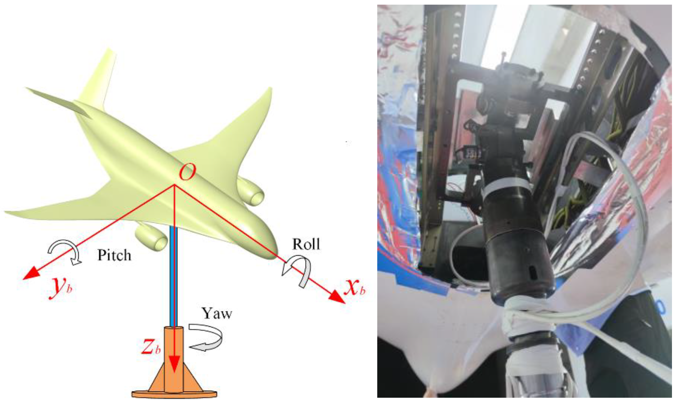
As shown in Figure 1, the test model is connected to a strut by a low friction 3-DOF rotation mechanism, with the connection point coinciding with the center of mass in the model so that the model is constrained by linear displacement but has 3 angular degrees in freedom of motion [19]. Ox_by_bz_b is the body coordinate system, and the sequence of rotations follows the conventional definition of the Euler angles. In addition, the geometrical configurations and dimensions of the test models are described in detail in Section 5 of this paper.

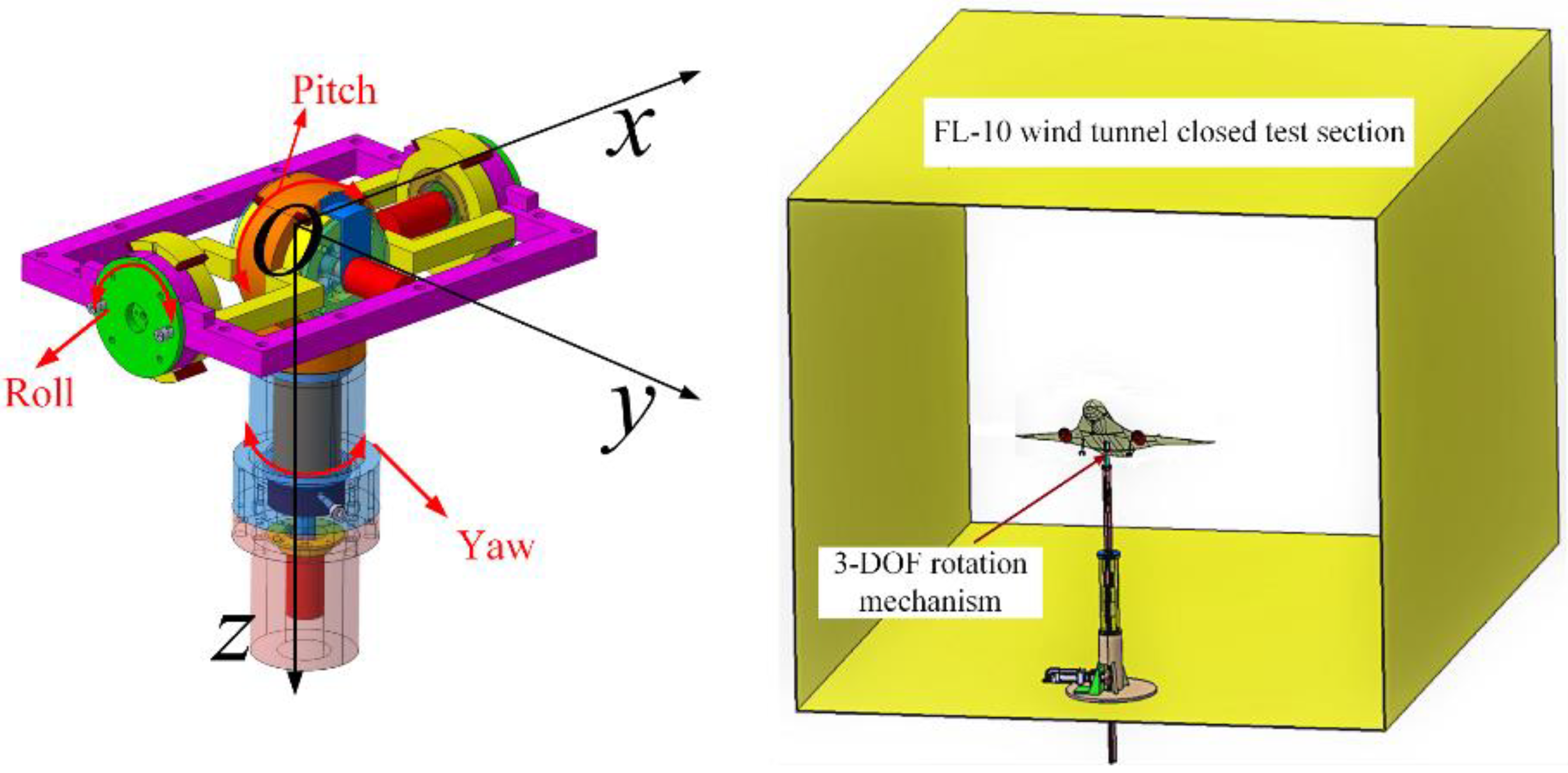
The 3-DOF rotation mechanism consists of three sets of rotating pairs, as shown in Figure 2, and the frictional force of the rotation device is negligible. The range of permitted rotation is ±45° in pitch and roll and ±180° in yaw.

The control surfaces on both sides of the V-tail of the test model are deflected in the same direction to provide the pitch moment [10]. The test model flies dynamically in the wind tunnel with onboard sensors installed on the model to measure the aircraft motion parameters and then uses the test measurement data for aerodynamic parameter identification. Note that in the actual flight test of a real aircraft, the lift and drag of the entire aircraft cannot be measured accurately. In the wind tunnel virtual flight test, a strain gauge balance is installed at the connection between the three-axis rotation mechanism and the center of mass of the aircraft, which can record the aerodynamic forces and the forces of the support rod on the model in real time [14]. The data of motions that can be directly measured in the wind tunnel test are shown in

Table 1. Measurable data from wind tunnel virtual flight test.

Parameters	Description	Instruments
ϕ, θ, ψ	Roll angle, pitch angle, and yaw angle	Inertial measurement unit
p, q, r	Roll rate, pitch rate, and yaw rate	Inertial measurement unit
α, β	Angle of attack and sideslip	Numerical solution
δe	V-tail longitudinal control surface deflection	Rotary encoder
Fx, Fz	Force of support device in the x- and z-axis directions (airflow coordinate system)	Strain gauge balance

.

2.1. Flight Dynamics Modeling

The following basic assumptions should be adopted when modeling flight dynamics and linearizing equations of motion:

• Ignore the curvature of the Earth and the rotation of the Earth;
• The aircraft is a rigid body with no elastic deformation and is symmetrical about the plane Ox_bz_b under the body’s coordinate system;
• When linearizing the equations of motion, the basic state of the aircraft is constant linear flight;
• The disturbances of force and moment relative to the reference motion can be represented by a first-order linear relationship.

Generally, the aircraft is symmetric about the Ox_bz_b plane in the body coordinate system; that is, I_xy = I_yz = 0. In the wind tunnel virtual flight test, the longitudinal rotation dynamics and kinematic equations of the model around the center of mass are the same as those of free flight, as shown in Equation (1) [20].

$$\{\begin{array}{l}M=I_y\dot{q}-I_{zx}\left(r^2-p^2\right)-\left(I_z-I_x\right)rp\\ \dot{\theta }=q\cos \varphi -r\sin \varphi \end{array}$$

(1)

where I_x, I_y, and I_z are the inertia of the three axes; I_xz is the cross inertia; p, q, and r are the roll rate, pitch rate, and yaw rate, respectively; and M is the pitch moment of the model in the body coordinate system.

In the wind tunnel virtual flight test, the longitudinal dynamic equation of the center of mass of an aircraft in the flight-path coordinate system is shown in Equation (2):

$$\{\begin{array}{l}m\frac{dV}{dt}=F_{x\_k}=0\\ -mV\frac{d\gamma }{dt}=F_{z\_k}=0\end{array}$$

(2)

where m is the mass of the model; γ is the climb angle; and F_{x_k} and F_{z_k} are the combined external forces on the aircraft under the x- and z-axis of the flight-path coordinate system, respectively. Since the model has no translational motion, the combined external force F_{x_k} = F_{z_k} = 0.

In the wind tunnel virtual flight test, the external forces on the model include gravity, the triaxial aerodynamic forces, and the force exerted by the support rod on the model. All external forces are transformed into the flight-path coordinate system, as shown in Equation (3):

$$\left[\begin{array}{c}{F}_{x\_k}\\ 0\\ F_{z\_k}\end{array}\right]=L_{ka}·\left[\begin{array}{c}-D\\ 0\\ -L\end{array}\right]+L_{kg}·\left[\begin{array}{c}0\\ 0\\ mg\end{array}\right]+L_{ka}·\left[\begin{array}{c}{F}_x\\ 0\\ F_z\end{array}\right]$$

(3)

where L_ka is the rotation matrix from the airflow coordinate system to the flight-path coordinate system; L_kg is the rotation matrix from the ground coordinate system to the flight-path coordinate system; L and D are the lift and drag forces of the model, respectively; and F_x and F_z are the forces of the support rod on the model in the x- and z-axis directions, respectively.

The combined external forces F_{x_k} and F_{z_k} of the model under the flight-path coordinate system obtained from Equation (3) are substituted into Equation (2) to obtain the dynamic equations of the center of mass, as shown in Equation (4):

$$\{\begin{array}{l}m\frac{dV}{dt}=F_{x\_k}=-D-mg\sin \gamma +F_x\\ -mV\frac{d\gamma }{dt}=F_{z\_k}=-L+mg\cos \gamma +F_z\end{array}$$

(4)

The angle of attack and sideslip are important parameters in aerodynamic parameters identification, and measurement accuracy directly affects the accuracy of the identification results. In real flight, α and β are usually measured by vane sensors, which often have a large measurement error due to airflow instability. However, in the wind tunnel virtual flight test, they can be solved directly by the attitude angle of the three axes. Due to the high accuracy of the attitude angle measurement, the accuracy of the solved angle of attack and sideslip is also high.

The origin O_g of the ground coordinate system is defined at the model center of mass, Ox_g points in the direction of wind speed, and Oz_g is vertically downward. In the wind tunnel test, the direction of the incoming flow is constant, resulting in the x-axis of the air coordinate system, ground coordinate system, and flight-path coordinate system all coinciding. Therefore, the component of airspeed in the body coordinate system can be calculated by using the attitude angle and the coordinate axis rotation matrix [21], and then the airflow angles α and β are directly solved, as shown in Equation (5):

$$\{\begin{array}{l}\left[\begin{array}{l}u\\ v\\ w\end{array}\right]=L_{bg}\left[\begin{array}{l}V\\ 0\\ 0\end{array}\right]=\left[\begin{array}{ccc}{a}_{11}& a_{12}& a_{13}\\ a_{21}& a_{22}& a_{23}\\ a_{31}& a_{32}& a_{33}\end{array}\right]\left[\begin{array}{l}V\\ 0\\ 0\end{array}\right]\\ a_{11}=\cos \theta \cos \psi \hspace{0.17em}\hspace{0.17em}\hspace{0.17em}\\ a_{21}=\sin \varphi \sin \theta \cos \psi -\cos \varphi \sin \psi \hspace{0.17em}\\ a_{31}=\cos \varphi \sin \theta \cos \psi +\sin \varphi \sin \psi \hspace{0.17em}\\ \alpha =\arctan (w/u)=\arctan (a_{31}/a_{11})\\ \beta =\arcsin (v/V)=\arcsin (a_{21})\end{array}$$

(5)

where u, v, and w are the components of airspeed in the body coordinate system and L_bg is the rotation matrix from the ground coordinate system to the body coordinate system.

2.2. Linearization and Decoupling for Equations of Motion

The motion of the model in the wind tunnel virtual flight test can be considered as the superposition of two parts of motion, namely, (a) the motion of free flight without support constraints and (b) the influence of the force exerted by the support rod on the motion of the model.

For linearization of the equations of motion, the disturbances of force and moment relative to the reference motion can be represented by a linear relationship [22], and ΔL, ΔD, and ΔM can be expressed as Equation (6):

$$\{\begin{array}{l}\Delta L=L_V\Delta V+L_{\alpha }\Delta \alpha +L_{\delta e}\Delta \delta e\\ \Delta D=D_V\Delta V+D_{\alpha }\Delta \alpha +D_{\delta e}\Delta \delta e\\ \Delta M=M_V\Delta V+M_{\alpha }\Delta \alpha +M_q\Delta q+M_{\dot{\alpha }}\Delta \dot{\alpha }+M_{\delta e}\Delta \delta e\end{array}$$

(6)

Since the model undergoes no translational motion, the resultant force of gravity, the aerodynamic force, and the force of the support rod is zero. Make the combined external forces F_{x_k} and F_{z_k} of the model in Equation (3) be 0, and the expressions of the forces F_x and F_z of the support rod can be obtained:

$$\{\begin{array}{l}{F}_x=D+mg\sin \gamma \\ F_z=L-mg\cos \gamma \end{array}$$

(7)

Equation (7) can be linearized with a reference state parameter of ${\gamma }_{*}$=0°, as shown in Equation (8).

$$\{\begin{array}{l}\Delta F_x=D_V\Delta V+(D_{\alpha }-mg)\Delta \alpha +mg\Delta \theta +D_{\delta e}\Delta \delta e\\ \Delta F_z=L_V\Delta V+L_{\alpha }\Delta \alpha +L_{\delta e}\Delta \delta e\end{array}$$

(8)

Here, ΔF_x and ΔF_z are expressed as a linear superposition of aerodynamic force and gravity. According to Equation (8), the linear expressions of supporting forces ΔF_x and ΔF_z can be obtained as:

$$\{\begin{array}{l}\Delta F_x=F_{x-}{}_V\Delta V+F_{x-}{}_{\alpha }\Delta \alpha +F_{x-}{}_{\theta }\Delta \theta +F_{x-}{}_{\delta e}\Delta \delta e\\ \Delta F_z=F_{z-}{}_V\Delta V+F_{z-}{}_{\alpha }\Delta \alpha +F_{z-}{}_{\delta e}\Delta \delta e\end{array}$$

(9)

Where F_x-V, F_x-α, F_x-θ, and F_x-δe denote the derivatives of the tangential force generated by the support rod with respect to the velocity, angle of attack, pitch angle, and elevator deflection in the airflow coordinate system, respectively; F_z-V, F_z-α and F_z-δe denote the derivatives of the normal force generated by the support rod with respect to the velocity, angle of attack, and elevator deflection, respectively; and the specific expressions are shown in Equation (10).

$$\{\begin{array}{l}{F}_{x-}{}_V=D_V\hspace{0.17em}\hspace{0.17em}\hspace{0.17em}\hspace{0.17em}\hspace{0.17em}\hspace{0.17em}\hspace{0.17em}\hspace{0.17em}\hspace{0.17em}\hspace{0.17em}\hspace{0.17em}\hspace{0.17em}\hspace{0.17em}{F}_{z-}{}_V=L_V\\ F_{x-}{}_{\alpha }=D_{\alpha }-mg\hspace{0.17em}\hspace{0.17em}\hspace{0.17em}\hspace{0.17em}\hspace{0.17em}\hspace{0.17em}{F}_{z-}{}_{\alpha }=L_{\alpha }\\ F_{x-}{}_{\theta }=mg\hspace{0.17em}\hspace{0.17em}\hspace{0.17em}\hspace{0.17em}\hspace{0.17em}\hspace{0.17em}\hspace{0.17em}\hspace{0.17em}\hspace{0.17em}\hspace{0.17em}\hspace{0.17em}\hspace{0.17em}\hspace{0.17em}{F}_{z-}{}_{\delta e}=L_{\delta e}\\ F_{x-}{}_{\delta e}=D_{\delta e}\end{array}$$

(10)

The longitudinal equations of motion for the wind tunnel virtual flight shown in Equations (1) and (4) are linearized, and substituting the expressions ΔL, ΔD, ΔM, ΔF_x, and ΔF_z shown in Equations (6) and (9) into the linearized equations, the linearization result for the equations of motion of the aircraft in steady state flight at $V_{*}$ and ${\alpha }_{*}$ are obtained as shown in Equation (11).

$$\begin{array}{l}\left[\begin{array}{c}\Delta \dot{V}\\ \Delta \dot{\alpha }\\ \Delta \dot{q}\\ \Delta \dot{\theta }\end{array}\right]=\underset{}{\underbrace{\left[\begin{array}{cccc}{X}_V& X_{\alpha }+g& 0& -g\\ -Z_V& -Z_{\alpha }& 1& 0\\ {\overline{M}}_V& {\overline{M}}_{\alpha }& {\overline{M}}_q+{\overline{M}}_{\dot{\alpha }}& 0\\ 0& 0& 1& 0\end{array}\right]}}\left[\begin{array}{c}\Delta V\\ \Delta \alpha \\ \Delta q\\ \Delta \theta \end{array}\right]+\underset{}{\underbrace{\left[\begin{array}{c}\frac{-D_{\delta e}}{m}\\ -\frac{L_{{\delta }_e}}{m{V}_{*}}\\ {\overline{M}}_{{\delta }_e}\\ 0\end{array}\right]}}\Delta {\delta }_e\\ \hspace{0.17em}\hspace{0.17em}\hspace{0.17em}\hspace{0.17em}\hspace{0.17em}\hspace{0.17em}\hspace{0.17em}\hspace{0.17em}\hspace{0.17em}\hspace{0.17em}\hspace{0.17em}\hspace{0.17em}\hspace{0.17em}\hspace{0.17em}\hspace{0.17em}\hspace{0.17em}\hspace{0.17em}\hspace{0.17em}\hspace{0.17em}\hspace{0.17em}\hspace{0.17em}\hspace{0.17em}\hspace{0.17em}\hspace{0.17em}\hspace{0.17em}\hspace{0.17em}\hspace{0.17em}\hspace{0.17em}\hspace{0.17em}\hspace{0.17em}{A}_1\hspace{0.17em}\hspace{0.17em}\hspace{0.17em}\hspace{0.17em}\hspace{0.17em}\hspace{0.17em}\hspace{0.17em}\hspace{0.17em}\hspace{0.17em}\hspace{0.17em}\hspace{0.17em}\hspace{0.17em}\hspace{0.17em}\hspace{0.17em}\hspace{0.17em}\hspace{0.17em}\hspace{0.17em}\hspace{0.17em}\hspace{0.17em}\hspace{0.17em}\hspace{0.17em}\hspace{0.17em}\hspace{0.17em}\hspace{0.17em}\hspace{0.17em}\hspace{0.17em}\hspace{0.17em}\hspace{0.17em}\hspace{0.17em}\hspace{0.17em}\hspace{0.17em}\hspace{0.17em}\hspace{0.17em}\hspace{0.17em}\hspace{0.17em}\hspace{0.17em}\hspace{0.17em}\hspace{0.17em}\hspace{0.17em}{B}_1\\ \hspace{0.17em}\hspace{0.17em}\hspace{0.17em}\hspace{0.17em}\hspace{0.17em}\hspace{0.17em}\hspace{0.17em}\hspace{0.17em}+\underset{}{\underbrace{\left[\begin{array}{cccc}\frac{D_V}{m}& \frac{D_{\alpha }}{m}-g& 0& g\\ \frac{L_V}{m{V}_{*}}& \frac{L_{\alpha }}{m{V}_{*}}& 0& 0\\ {\overline{M}}_{\dot{\alpha }}\frac{L_V}{m{V}_{*}}& {\overline{M}}_{\dot{\alpha }}\frac{L_{\alpha }}{m{V}_{*}}& 0& 0\\ 0& 0& 0& 0\end{array}\right]}}\left[\begin{array}{c}\Delta V\\ \Delta \alpha \\ \Delta q\\ \Delta \theta \end{array}\right]+\underset{}{\underbrace{\left[\begin{array}{c}\frac{D_{\delta e}}{m}\\ \frac{L_{\delta e}}{m{V}_{*}}\\ {\overline{M}}_{\dot{\alpha }}\frac{L_{\delta e}}{m{V}_{*}}\\ 0\end{array}\right]}}\Delta {\delta }_e\\ \hspace{0.17em}\hspace{0.17em}\hspace{0.17em}\hspace{0.17em}\hspace{0.17em}\hspace{0.17em}\hspace{0.17em}\hspace{0.17em}\hspace{0.17em}\hspace{0.17em}\hspace{0.17em}\hspace{0.17em}\hspace{0.17em}\hspace{0.17em}\hspace{0.17em}\hspace{0.17em}\hspace{0.17em}\hspace{0.17em}\hspace{0.17em}\hspace{0.17em}\hspace{0.17em}\hspace{0.17em}\hspace{0.17em}\hspace{0.17em}\hspace{0.17em}\hspace{0.17em}\hspace{0.17em}\hspace{0.17em}{A}_2\hspace{0.17em}\hspace{0.17em}\hspace{0.17em}\hspace{0.17em}\hspace{0.17em}\hspace{0.17em}\hspace{0.17em}\hspace{0.17em}\hspace{0.17em}\hspace{0.17em}\hspace{0.17em}\hspace{0.17em}\hspace{0.17em}\hspace{0.17em}\hspace{0.17em}\hspace{0.17em}\hspace{0.17em}\hspace{0.17em}\hspace{0.17em}\hspace{0.17em}\hspace{0.17em}\hspace{0.17em}\hspace{0.17em}\hspace{0.17em}\hspace{0.17em}\hspace{0.17em}\hspace{0.17em}\hspace{0.17em}\hspace{0.17em}\hspace{0.17em}\hspace{0.17em}\hspace{0.17em}{B}_2\end{array}$$

(11)

where A₁ and B₁ represent the free flight longitudinal stability matrix and the control matrix of the control surface, respectively, and A₂ represents the matrix of the additional motion of the model caused by the support force. Since the control surface deflection produces lift, drag, and pitch moments, the constraint of the support rod has an impact on the control matrix, as shown in B₂. The expressions of the longitudinal dynamic derivatives in Equation (11) are shown in

Table 2. Longitudinal dynamic derivatives.

Dynamic Derivatives	Composition	Dynamic Derivatives	Composition
${\overline{M}}_V$	$\frac{M_V}{I_y}–\frac{M_{\dot{\alpha }}}{I_y}\frac{L_V}{{mV}_{*}}$	${\overline{M}}_{\alpha }$	$\frac{M_{\alpha }}{I_y}–\frac{M_{\dot{\alpha }}}{I_y}\frac{L_{\alpha }}{{mV}_{*}}$
${\overline{M}}_q+{\overline{M}}_{\dot{\alpha }}$	$\frac{{\overline{M}}_q+{\overline{M}}_{\dot{\alpha }}}{I_y}$	${\overline{M}}_{\delta e}$	$\frac{M_{\delta e}}{I_y}–\frac{M_{\dot{\alpha }}}{I_y}\frac{L_{\delta e}}{{\mathit{mV}}_{*}}$
MV	${\overline{q}}_{*}{\mathit{ScC}}_{\mathit{mV}}/V_{*}$	Mα	${\overline{q}}_{*}{\mathit{ScC}}_{m\alpha }$
Mq	${\overline{q}}_{*}{\mathit{Sc}}^2{C}_{mq}/{2V}_{*}$	$M_{\dot{\alpha }}$	${\overline{q}}_{*}{\mathit{Sc}}^2{C}_{m\dot{\alpha }}$$/{2V}_{*}$
Mδe	${\overline{q}}_{*}{\mathit{ScC}}_{m\delta e}/I_y$	XV	$-$DV/m
Xα	$-$$(D_{*}$$\tan {\alpha }_{*}$ + Dα)/m	ZV	$L_V/m{V}_{*}$
Zα	$(L_{\alpha }+D_{*}$$)/m{V}_{*}$	DV	${\overline{q}}_{*}S(C_{\mathit{DV}}+2C_{D*})/V_{*}$
Dα	${\overline{q}}_{*}S{C}_{D\alpha }$	Dδe	${\overline{q}}_{*}S{C}_{D\delta e}$
LV	${\overline{q}}_{*}S(C_{LV}+2C_{L*})$	Lα	${\overline{q}}_{*}S{C}_{L\alpha }$
Lδe	${\overline{q}}_{*}S{C}_{L\delta E}$

:

To simulate the motion of the aircraft in free flight through the aerodynamic parameter identification results of the wind tunnel virtual flight test, it is necessary to eliminate the influence of the A₂ and B₂ matrices in Equation (11). To simplify the description, Equation (11) is rewritten into the form shown in Equation (12). The mathematical expressions in the box are the differences in longitudinal equations of motion between wind tunnel virtual flight and free flight.

$$\begin{array}{l}\left[\begin{array}{c}\Delta \dot{V}\\ \Delta \dot{\alpha }\\ \Delta \dot{q}\\ \Delta \dot{\theta }\end{array}\right]=\underset{}{\underbrace{\left[\begin{array}{cccc}-\frac{D_V}{m}+\boxed{\frac{D_V}{m}}& \frac{D_{\alpha }}{m}+g+\boxed{\frac{D_{\alpha }}{m}-g}& 0& -g+\boxed{g}\\ -\frac{L_V}{m{V}_{*}}+\boxed{\frac{L_V}{m{V}_{*}}}& -\frac{L_{\alpha }}{m{V}_{*}}+\boxed{\frac{L_{\alpha }}{m{V}_{*}}}& 1& 0\\ {\overline{M}}_V+\boxed{{\overline{M}}_{\dot{\alpha }}\frac{L_V}{m{V}_{*}}}& {\overline{M}}_{\alpha }+\boxed{{\overline{M}}_{\dot{\alpha }}\frac{L_{\alpha }}{m{V}_{*}}}& {\overline{M}}_q+{\overline{M}}_{\dot{\alpha }}& 0\\ 0& 0& 1& 0\end{array}\right]}}\left[\begin{array}{c}\Delta V\\ \Delta \alpha \\ \Delta q\\ \Delta \theta \end{array}\right]+\underset{}{\underbrace{\left[\begin{array}{c}\frac{-D_{\delta e}}{m}+\boxed{\frac{D_{\delta e}}{m}}\\ -\frac{L_{{\delta }_e}}{m{V}_{*}}+\boxed{\frac{L_{\delta e}}{m{V}_{*}}}\\ {\overline{M}}_{{\delta }_e}+\boxed{{\overline{M}}_{\dot{\alpha }}\frac{L_{\delta e}}{m{V}_{*}}}\\ 0\end{array}\right]}}\Delta {\delta }_e\\ \hspace{0.17em}\hspace{0.17em}\hspace{0.17em}\hspace{0.17em}\hspace{0.17em}\hspace{0.17em}\hspace{0.17em}\hspace{0.17em}\hspace{0.17em}\hspace{0.17em}\hspace{0.17em}\hspace{0.17em}\hspace{0.17em}\hspace{0.17em}\hspace{0.17em}\hspace{0.17em}\hspace{0.17em}\hspace{0.17em}\hspace{0.17em}\hspace{0.17em}\hspace{0.17em}\hspace{0.17em}\hspace{0.17em}\hspace{0.17em}\hspace{0.17em}\hspace{0.17em}\hspace{0.17em}\hspace{0.17em}\hspace{0.17em}\hspace{0.17em}\hspace{0.17em}\hspace{0.17em}\hspace{0.17em}\hspace{0.17em}\hspace{0.17em}\hspace{0.17em}\hspace{0.17em}\hspace{0.17em}\hspace{0.17em}\hspace{0.17em}\hspace{0.17em}\hspace{0.17em}\hspace{0.17em}\hspace{0.17em}\hspace{0.17em}\hspace{0.17em}\hspace{0.17em}A\hspace{0.17em}\hspace{0.17em}\hspace{0.17em}\hspace{0.17em}\hspace{0.17em}\hspace{0.17em}\hspace{0.17em}\hspace{0.17em}\hspace{0.17em}\hspace{0.17em}\hspace{0.17em}\hspace{0.17em}\hspace{0.17em}\hspace{0.17em}\hspace{0.17em}\hspace{0.17em}\hspace{0.17em}\hspace{0.17em}\hspace{0.17em}\hspace{0.17em}\hspace{0.17em}\hspace{0.17em}\hspace{0.17em}\hspace{0.17em}\hspace{0.17em}\hspace{0.17em}\hspace{0.17em}\hspace{0.17em}\hspace{0.17em}\hspace{0.17em}\hspace{0.17em}\hspace{0.17em}\hspace{0.17em}\hspace{0.17em}\hspace{0.17em}\hspace{0.17em}\hspace{0.17em}\hspace{0.17em}\hspace{0.17em}\hspace{0.17em}\hspace{0.17em}\hspace{0.17em}\hspace{0.17em}\hspace{0.17em}\hspace{0.17em}\hspace{0.17em}\hspace{0.17em}\hspace{0.17em}\hspace{0.17em}\hspace{0.17em}\hspace{0.17em}\hspace{0.17em}\hspace{0.17em}\hspace{0.17em}\hspace{0.17em}\hspace{0.17em}\hspace{0.17em}\hspace{0.17em}\hspace{0.17em}B\end{array}$$

(12)

According to Equation (12), the aerodynamic parameters identification model for the wind tunnel virtual flight test can be established. Since the displacement of the model is constrained, the lift and drag derivatives cannot be directly identified by the motions of the model. In addition, since the wind speed in the wind tunnel is fixed for each test, the velocity derivatives need to be solved separately. It is necessary to establish a step-by-step identification method for the lift, drag derivatives, pitch moment derivatives, and velocity derivatives. In addition, Equation (12) indicates differences between each aerodynamic derivative of wind tunnel virtual flight and free flight, and the identification results need to be corrected to obtain accurate aerodynamic derivatives of free flight.

3. Design Method for Excitation Signals Based on Identifiable Requirements

The most commonly used excitation signals include the dipole square wave, 3211 multipole square wave, sine wave, and frequency swept signals [23]. Since the closed-loop control law has a significant feedback effect on the input excitation signal, large differences can arise between the actual deflection angle of the control surface and the input excitation signal. Compared to other excitation signals, the control system has the minimal effect on the swept signal, so the swept signal was suggested in reference [24] as the excitation signal for the identification of longitudinal aerodynamic parameters of the aircraft with control augmentation laws.

In this article, an excitation signal parameter design method based on frequency domain analysis is proposed to design the frequency band and amplitude of the excitation signal. The equations of motion of the model are established based on the force measurement data from the conventional wind tunnel, and the amplitude–frequency response of the parameters to be identified with the frequency change of the excitation signal is observed by Bode diagram analysis for the aircraft equations of motion. The frequency range of the excitation signal is determined by ensuring that the amplitude response of the aerodynamic coefficients caused by each motion variable (α, q, V, and θ) and operation variable (δ_e) are large. Finally, the amplitude of the excitation signal is adjusted to ensure that the signal contains high energy in the frequency band of interest.

The design parameters of the swept frequency signal include the lower frequency limit ω_l, the upper limit ω_h, and the signal amplitude |A|. Equation (13) is the observation equation for the longitudinal motions of the aircraft, which contains the observation equations for the lift, drag, and pitch moment.

$$\{\begin{array}{l}\Delta L=L_{\alpha }\Delta \alpha +L_{\delta e}\Delta {\delta }_e\\ \Delta D=D_{\alpha }\Delta \alpha +D_{\delta e}\Delta {\delta }_e\\ \Delta \dot{q}=M_{\alpha }\Delta \alpha +(M_q+M_{\dot{\alpha }})\Delta q+M_{{\delta }_e}\Delta {\delta }_e\end{array}$$

(13)

In Equation (13), the longitudinal parameters to be identified are M_α, $M_q{+M}_{\dot{\alpha }}$, M_δe, L_α, L_δe, D_α, and D_δe. In the wind tunnel virtual flight test, the pitch angle θ is approximately equal to the angle of attack α because the model has no track change. Therefore, the two derivatives of $M_q$ and $M_{\dot{\alpha }}$ cannot be identified separately in the identification of aerodynamic parameters but can only be identified as a whole, $M_q{+M}_{\dot{\alpha }}$.

Based on Equation (13), amplitude–frequency response curves (|M_α(ω)/δ_e|, |$M_q{+M}_{\dot{\alpha }}$(ω)/δ_e|, |M_δe(ω)/δ_e|, and |Δ$\dot{q}$(ω)/δ_e|) of M_α, $M_q{+M}_{\dot{\alpha }}$, M_δe, and Δ $\dot{q}$ with the variation of the longitudinal excitation signal frequency can be drawn according to the pitch moment observation equation; amplitude–frequency response curves (|L_α(ω)/δ_e|, |L_δe(ω)/δ_e|, and |ΔL(ω)/δ_e|) of L_α, L_δe, and ΔL with the frequency of the excitation signal can be drawn according to the lift observation equation; and amplitude–frequency response curves (|D_α(ω)/δ_e|, |D_δe(ω)/δ_e|, and |ΔD(ω)/δ_e|) of D_α, D_δe, and ΔD with the frequency of the excitation signal can be drawn according to the drag observation equation.

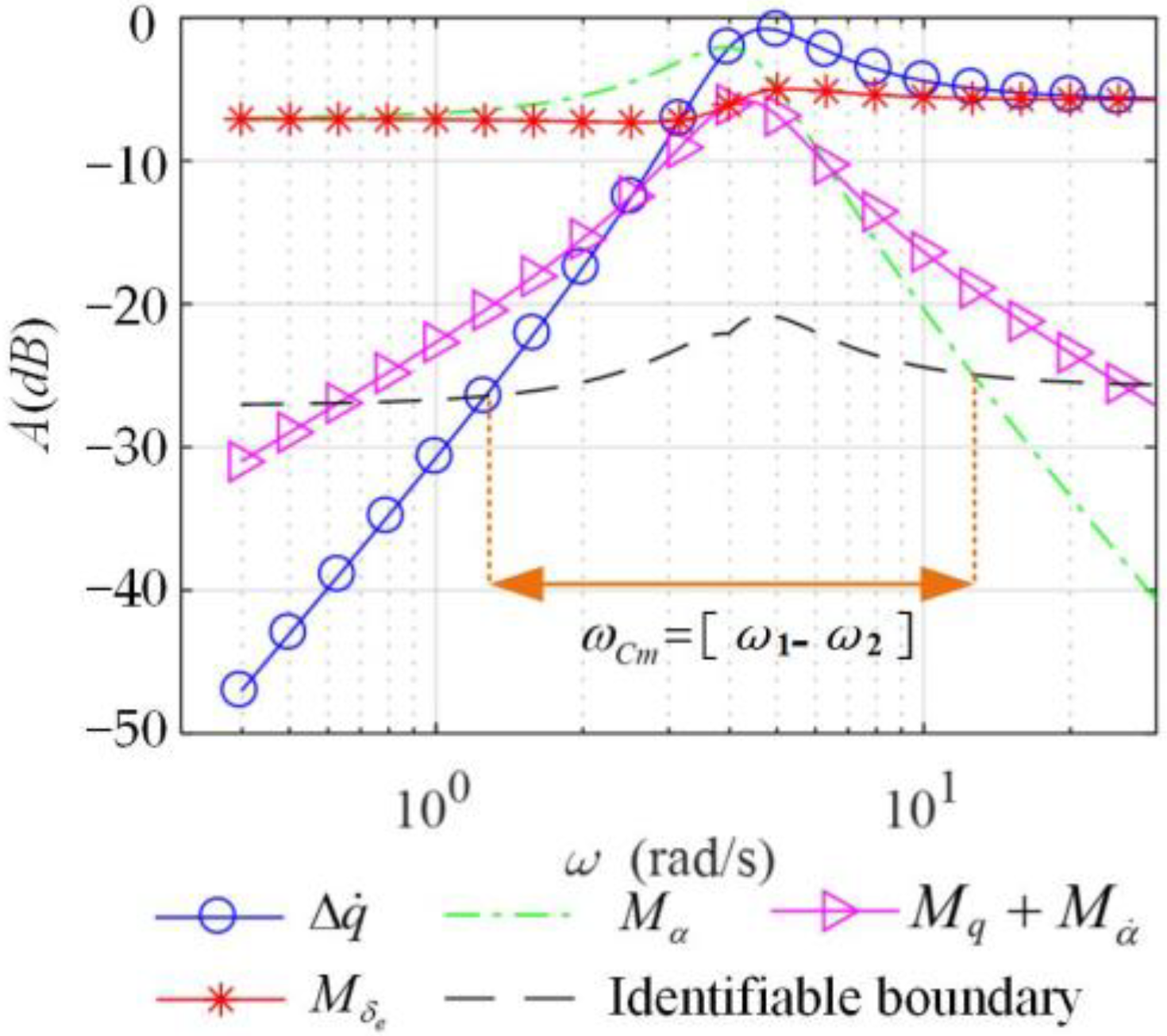
Figure 3 shows the amplitude–frequency characteristic curve of each pitch moment parameter with the frequency of the excitation signal; the amplitude–frequency characteristic curve of lift and drag derivatives can be obtained in the same way. The frequency at the resonance peak is approximately equal to the short-period mode frequency of the aircraft. When the excitation signal frequency is lower or higher than the short-period frequency, the response amplitude of each pitch moment parameter decreases.

To ensure the identifiability of each pitch moment derivative, the magnitude–frequency response magnitudes of the moment coefficient M_αΔα caused by the change in the angle of attack, the moment coefficient ($M_q{+M}_{\dot{\alpha }}$)Δq caused by the pitch rate, the moment coefficient M_δeΔδ_e caused by the control surface deflection, and the pitch rate acceleration Δ$\dot{q}$ should not differ significantly.

In the same way, for the lift observation equation in Equation (13), the magnitude–frequency response magnitudes of the lift introduced by the change in the angle of attack L_αΔα, the lift introduced by the control surface deflection L_δeΔδ_e, and the total lift change ΔL should not differ significantly. The magnitude response magnitudes of the drag introduced by the change in the angle of attack D_αΔα, the drag introduced by the control surface deflection D_δeΔδ_e, and the total drag variation ΔD in the drag observation equation should also not differ significantly.

Reference [25] noted that the aerodynamic derivative is considered to be identifiable when the proportion of the motion response component caused by each aerodynamic derivative is at least 10% of the total motion response. We calculate the sum of the response amplitudes corresponding to each aerodynamic derivative at all frequencies in the Bode diagram and obtain the value corresponding to 1/10 of the total response amplitude, as shown in Equation (14).

$$\{\begin{array}{l}{\left|A\right|}_{Cm-{\omega }_i}=\frac{1}{10}{\displaystyle \sum _{{\omega }_i}\left({\left|A\right|}_{M_{\alpha }}+{\left|A\right|}_{M_q+M_{\dot{\alpha }}}+{\left|A\right|}_{M_{{\delta }_e}}+{\left|A\right|}_{\dot{q}}\right)}\\ {\left|A\right|}_{CL-{\omega }_i}=\frac{1}{10}{\displaystyle \sum _{{\omega }_i}\left({\left|A\right|}_{L_{\alpha }}+{\left|A\right|}_{L_{{\delta }_e}}+{\left|A\right|}_{\Delta L}\right)}\\ {\left|A\right|}_{CD-{\omega }_i}=\frac{1}{10}{\displaystyle \sum _{{\omega }_i}\left({\left|A\right|}_{D_{\alpha }}+{\left|A\right|}_{D_{{\delta }_e}}+{\left|A\right|}_{\Delta D}\right)}\end{array}$$

(14)

where ${\left|A\right|}_{M_{\alpha }}$, ${\left|A\right|}_{M_q{+M}_{\dot{\alpha }}}$, ${\left|A\right|}_{M_{\delta e}}$, ${\left|A\right|}_{\dot{q}}$ and are the Bode response amplitudes of each pitch moment coefficient at the excitation signal frequency of ω_i; ${\left|A\right|}_{L_{\alpha }}$, ${\left|A\right|}_{L_{\delta e}}$, and ${\left|A\right|}_{\Delta L}$ are the response amplitudes of each lift component; and ${\left|A\right|}_{D_{\alpha }}$, ${\left|A\right|}_{D_{\delta e}}$, and ${\left|A\right|}_{\Delta D}$ are the response amplitudes of each drag component. ${\left|A\right|}_{{\mathit{Cm}-\omega }_i}$, ${\left|A\right|}_{{\mathit{CL}-\omega }_i}$, and ${\left|A\right|}_{{\mathit{CD}-\omega }_i}$ are 1/10 of the total response amplitude of the pitch moment, lift, and drag at an excitation signal frequency of ω_i, respectively.

According to Equation (14), 1/10 of the total response amplitudes of the pitch moment, lift, and drag under different frequency excitation signals can be calculated and connected into a curve. The dashed line in Figure 3 is the demarcation line corresponding to the total pitch moment response amplitude of 1/10, which is defined as the identifiable boundary of the pitch moment derivatives for different frequency excitation signals. The same method can be used to obtain the identifiable boundaries of lift and drag derivatives.

When the response amplitude corresponding to an aerodynamic derivative is above the identifiable boundary, the derivative is identifiable at this frequency; otherwise, it is not identifiable. When the frequency is in the range of ${\omega }_{\mathit{Cm}}$ $\in$[ω₁~ω₂] in Figure 3, i.e., the amplitude responses of all moment derivatives to be identified are above the identifiable boundary, then all longitudinal pitch moment derivatives are identifiable. Thus, the frequency range of interest for the excitation signal determined by the pitch moment derivative is ${\omega }_{\mathit{Cm}}$.

In the same way, the attention frequency range of excitation signals ${\omega }_{\mathit{CL}}$ and ${\omega }_{\mathit{CD}}$ determined by the lift and drag derivatives can be obtained. To ensure the accuracy of identification of all longitudinal aerodynamic derivatives, it is necessary to take the intersection of ${\omega }_{\mathit{Cm}}$, ${\omega }_{\mathit{CL}}$, and ${\omega }_{\mathit{CD}}$ to obtain the frequency band of interest ω of the longitudinal excitation signal, i.e., ω = ${\omega }_{\mathit{Cm}}$$\cap$${\omega }_{\mathit{CL}}$$\cap$${\omega }_{\mathit{CD}}$.

The amplitude of the excitation signal should be designed within a suitable range. If the excitation signal amplitude is too large, the angle of attack of the aircraft will vary too much, which will introduce nonlinear aerodynamic effects; if the amplitude is too small, it is not easy to excite the aircraft’s motion mode, and the flight state parameters are also more susceptible to noise interference, thus affecting the data accuracy. Therefore, first, it is necessary to ensure that the variation range of the aircraft’s angle of attack is approximately ±2° and that the aerodynamic derivatives are in the linear region. Then, under the premise of considering the influence of the feedback of the flight control system, the amplitude of the excitation signal is determined according to the requirements of the change in the angle of attack.

4. Step-By-Step Identification and Correction Method for the Aerodynamic Parameters

In actual flight, changes in lift and drag bring about changes in speed and trajectory, so the lift and drag derivatives of the model can be identified by the equations for free flight motion [26]. However, during the wind tunnel virtual flight test, the model has no speed and track changes, so the lift and drag derivatives cannot be identified through the equations of motion. Lift and drag forces need to be identified separately by other methods.

In the wind tunnel virtual flight test, the pitch moment derivatives can be identified by the pitch equation of motion. However, Equation (12) shows that due to the constraint of displacement, the pitch equations of motion between wind tunnel virtual flight and free flight are different, so it is necessary to correct the pitch moment derivatives obtained by identification.

In addition, since the wind speed is fixed during the wind tunnel test, the velocity derivatives cannot be obtained directly by identification. Next, the step-by-step identification and correction methods for the lift and drag derivatives, pitch moment derivatives, and velocity derivatives are introduced.

4.1. Identification Method for the Lift and Drag Derivatives

In the wind tunnel virtual flight test, a strain gauge balance is installed at the center of mass of the model, which can measure the lift and drag of the entire aircraft in real time. Therefore, the measurements of lift L and drag D can be regarded as observed variables to identify the derivatives of aerodynamic forces. The identification model for the lift and drag derivatives is shown in Equation (15):

$$\{\begin{array}{l}{L}_m=L_{\hspace{0.17em}*}+L_{\alpha }\Delta \alpha +L_{\delta e}\Delta {\delta }_e\\ D_m=D_{\hspace{0.17em}*}+D_{\alpha }\Delta \alpha +D_{\delta e}\Delta {\delta }_e\end{array}$$

(15)

where L_m and D_m are the lift and drag of the test model directly measured by the strain balance; Δα and Δδ_e are the change in the angle of attack and the V-tail control surface deflection, which can be measured directly by the sensor. The parameters to be identified are Θ = [$L_{*}$, L_α, L_δe, $D_{*}$, D_α, D_δe].

Since the lift and drag forces measured by the balance are the actual aerodynamic forces on the model without the force of the support rod, the identification results based on the measured data are the lift and drag derivatives of free flight.

For the lift and drag observation equations shown in Equation (15), the derivatives can be directly identified using the least squares method. The general form of least squares identification is shown in Equation (16) [27]:

$$\{\begin{array}{l}y=X\Theta \\ z=X\Theta +v\end{array}$$

(16)

where Θ is the parameter to be identified; y is the theoretical output of the identification model; z is the actual observed value; X is a matrix of independent variables consisting of parameters such as motion variables (α, q, V, θ) and maneuvering variables (δ_e) of the aircraft; and v is the measurement noise matrix of the test device. In the wind tunnel test, the measurement accuracy of the strain balance is high, and v can be regarded as white noise with a mean value of 0, as shown in Equation (17):

$$\{\begin{array}{l}E(v)=0\\ E(v{v}^T)={\sigma }^{2}I\end{array}$$

(17)

The least squares solutions of the aerodynamic lift and drag derivatives to be identified are:

$$\widehat{\Theta }={(X^{T}X)}^{-1}{X}^{T}z$$

(18)

4.2. Identification and Correction Method for Pitch Moment Derivatives

According to Equation (12), there is a difference between the longitudinal equations of motion of the wind tunnel virtual flight and the free flight. The pitch moment derivatives obtained from the identification need to be corrected to obtain the derivatives for free flight. The state equation of longitudinal pitch motion in the wind tunnel virtual flight test is shown in Equation (19):

$$\{\begin{array}{l}\Delta \dot{V}=0\\ \Delta \dot{\alpha }=\Delta q\\ \Delta \dot{\theta }=\Delta q\\ \Delta \dot{q}={\tilde{M}}_{\alpha }\Delta \alpha +({\tilde{M}}_q+{\tilde{M}}_{\dot{\alpha }})\Delta q+{\tilde{M}}_{{\delta }_e}\Delta {\delta }_e\end{array}$$

(19)

The experimentally measured ΔV_m, Δα_m, Δθ_m, and Δq_m are selected as observation variables and the observation equation is shown in Equation (20):

$$\{\begin{array}{l}\Delta V_m=\Delta V+v_V\\ \Delta {\alpha }_m\hspace{0.17em}\hspace{0.17em}=\Delta \alpha +v_{\alpha }\\ \Delta {\theta }_m\hspace{0.17em}\hspace{0.17em}=\Delta \theta +v_{\theta }\\ \Delta q_m=\Delta q+v_q\end{array}$$

(20)

where ΔV, Δα, Δθ, and Δq are theoretical outputs; $v_V$, $v_{\alpha }$, $v_{\theta }$, and are $v_q$ measurement noise. The parameters to be identified are ${\tilde{M}}_{\alpha },{\tilde{M}}_q,{\tilde{M}}_{\dot{\alpha }}\mathrm{and}{\tilde{M}}_{\delta e}$.

For the parameter identification of the nonlinear models shown in Equations (19) and (20), the most commonly used method is the output error method based on maximum likelihood estimation [28]. The nonlinear dynamic equations can be expressed in the form shown in Equation (21):

$$\{\begin{array}{l}\dot{x}(t)\hspace{0.17em}\hspace{0.17em}=f[x(t),u(t),\Theta ]\hspace{0.17em}\hspace{0.17em}\hspace{0.17em}\hspace{0.17em}\hspace{0.17em}x(t_0)=x_0\\ y(t)\hspace{0.17em}\hspace{0.17em}=g[x(t),u(t),\Theta ]\\ z(t_k)=y(t_k)+v(t_k)\end{array}$$

(21)

where x is the state variable; u is the input variable; y is the output variable; z is the observed variable; f and g are the general nonlinear functions, which refer to Equations (19) and (20); and Θ is the parameter to be identified. Assume that the measurement noise v is Gaussian white noise with zero mean and a covariance matrix of R.

The purpose of parameter identification is to estimate the parameters Θ from the nonlinear model shown in Equation (21) according to the input u and the observed value z of the system. The output error method constructs a likelihood function J(θ,R) with the observed data and the unknown parameters as independent variables, as shown in Equation (22), and solves for the parameters to be identified by finding the extreme values of the likelihood function.

$$J(\Theta ,R)=\frac{1}{2}{\displaystyle \sum _{k=1}^N{[z(t_k)-y(t_k)]}^T{R}^{-1}[z(t_k)-y(t_k)]}+\frac{N}{2}In\left|R\right|$$

(22)

Starting from the specified initial value Θ₀, the Gauss–Newton solution algorithm shown in Equation (23) is used to iterate to find the optimal parameters to be identified.

$$\{\begin{array}{l}{\Theta }_{i+1}={\Theta }_i+\Delta \Theta \\ \Delta \Theta =-\frac{{\displaystyle \sum _{k=1}^N{\left[\frac{\partial y(t_k)}{\partial \Theta }\right]}^T{R}^{-1}\left[z(t_k)-y(t_k)\right]}}{{\displaystyle \sum _{k=1}^N{\left[\frac{\partial y(t_k)}{\partial \Theta }\right]}^T{R}^{-1}\left[\frac{\partial y(t_k)}{\partial \Theta }\right]}}\end{array}$$

(23)

The ${\tilde{M}}_{\alpha },{\tilde{M}}_q+{\tilde{M}}_{\dot{\alpha }} \mathrm{and} {\tilde{M}}_{\delta e}$ derivatives are obtained based on maximum likelihood identification. For the experimental model in this study, the damping moment derivative of lag of wash $M_{\dot{\alpha }}$ is approximately half of the pitch damping derivative ${\tilde{M}}_q$; that is, ${\tilde{M}}_{\dot{\alpha }}$ = 0.5${\tilde{M}}_q$.

According to Equation (12), there are differences between the pitch moment derivatives ${\tilde{M}}_{\alpha }$ and ${\tilde{M}}_{\delta e}$ obtained based on wind tunnel virtual flight test identification and the moment derivatives ${\overline{M}}_{\alpha }$ and ${\overline{M}}_{\delta e}$ corresponding to free flight, as shown in Equation (24):

$$\{\begin{array}{l}{\overline{M}}_{\alpha }={\tilde{M}}_{\alpha }-\boxed{{\tilde{M}}_{\dot{\alpha }}\frac{L_{\alpha }}{m{V}_{*}}}\\ {\overline{M}}_{{\delta }_e}={\tilde{M}}_{{\delta }_e}-\boxed{{\tilde{M}}_{\dot{\alpha }}\frac{L_{\delta e}}{m{V}_{*}}}\end{array}$$

(24)

After the pitch moment derivatives ${\tilde{M}}_{\alpha }$ and ${\tilde{M}}_{\delta e}$ are identified by the wind tunnel virtual flight test, the pitch moment derivatives ${\overline{M}}_{\alpha }$ and ${\overline{M}}_{\delta e}$ in free flight are obtained by subtracting the mathematical expressions in the boxes of Equation (24).

The parameters that can be obtained through the identification and correction of aerodynamic derivatives are Θ = [$L_{*}$, L_α, L_δe, $D_{*}$, D_α, D_δe, ${\overline{M}}_{\alpha }$, ${\overline{M}}_q$ + ${\overline{M}}_{\dot{\alpha }}$, $\overline{M}{\delta }_e$].

4.3. Solution and Correction Method for Velocity Derivatives

The wind speed at each wind tunnel test is fixed, so the velocity derivatives D_V, L_V, and ${\tilde{M}}_v$ cannot be directly identified by a single test. Therefore, it is necessary to solve the velocity derivatives through the test results under different wind speeds.

The wind tunnel virtual flight test is carried out at a certain equilibrium speed, angle of attack, and V-tail control surface deflection (V₁, α₁, and δ_e1) to measure the lift L₁ and drag D₁ of the whole aircraft at a state of static equilibrium. Then, the excitation signal is input to the control surface of the model and the dynamic motion data are measured. The lift and drag derivatives L_α, L_δe, D_δe, and D_α are identified by the least squares method, and the pitch moment derivatives ${\tilde{M}}_{\alpha }$ and ${\tilde{M}}_{\delta e}$ are identified by the maximum likelihood method. In addition, at another wind speed V₂, the model’s trim angle of attack α₂, lift L₂, drag D₂, and V-tail control surface deflection δ_e2 under the airflow coordinate system are all measurable. The data obtained from the two experiments are shown in

Table 3. Parameters for the velocity derivatives’ solution.

Serial No.	First Test	Second Test
Measured parameters	V1, α1, δe1 L1, D1	V2, α2, δe2 L2, D2
Identified parameters	Lα, Lδe, Dα, Dδe ${\stackrel{\sim }{M}}_{\alpha },{\stackrel{\sim }{M}}_{\delta e}$	-

.

Considering the existence of velocity derivatives, the model can be balanced at two state points with different velocities. According to the force and pitch moment balance of the model, the relationship shown in Equation (25) can be established:

$$\{\begin{array}{l}{D}_1+D_{\alpha }·({\alpha }_2-{\alpha }_1)+D_V·(V_2-V_1)+D_{\delta e}·({\delta }_{e2}-{\delta }_{e1})=D_2\\ L_1+L_{\alpha }·({\alpha }_2-{\alpha }_1)+L_V·(V_2-V_1)+L_{\delta e}·({\delta }_{e2}-{\delta }_{e1})=L_2\\ {\tilde{M}}_{\alpha }·({\alpha }_2-{\alpha }_1)+{\tilde{M}}_V·(V_2-V_1)+{\tilde{M}}_{{\delta }_e}·({\delta }_{e2}-{\delta }_{e1})=0\end{array}$$

(25)

The first line in Equation (25) is the equilibrium equation for the drag force, which is D₁ of the model under the first test and D₂ under the second test. The amount of change in drag is caused by changes in the angle of attack D_α(α₂ − α₁), control surface deflection D_δe(δ_e2 − δ_e1), and speed D_V(V₂ − V₁). In the same way, the balance equation of the lift and pitch moment can also be written.

The velocity derivatives D_V, L_V, and ${\tilde{M}}_v$ can be solved according to Equation (25), as shown in Equation (26):

$$\{\begin{array}{l}{D}_V=\frac{(D_2-D_1)-D_{\alpha }·({\alpha }_2-{\alpha }_1)-D_{\delta e}·({\delta }_{e2}-{\delta }_{e1})}{V_2-V_1}\\ L_V=\frac{(L_2-L_1)-L_{\alpha }·({\alpha }_2-{\alpha }_1)-L_{\delta e}·({\delta }_{e2}-{\delta }_{e1})}{V_2-V_1}\\ {\tilde{M}}_V=-\frac{{\tilde{M}}_{\alpha }·({\alpha }_2-{\alpha }_1)+{\tilde{M}}_{{\delta }_e}·({\delta }_{e2}-{\delta }_{e1})}{V_2-V_1}\end{array}$$

(26)

According to Equation (12), there is a difference between the velocity derivative ${\tilde{M}}_v$ obtained based on the wind tunnel virtual flight test and the velocity derivative of free flight ${\overline{M}}_v$, as shown in Equation (27):

$${\overline{M}}_V={\tilde{M}}_V-\boxed{{\tilde{M}}_{\dot{\alpha }}\frac{L_V}{m{V}_{*}}}$$

(27)

Therefore, after the velocity derivative ${\tilde{M}}_V$ is calculated through the wind tunnel virtual flight test, the velocity derivative ${\overline{M}}_V$ in free flight can be obtained by subtracting the mathematical expression in the box of Equation (27).

Based on the analysis in Section 4, it is clear that the displacement constraints lead to inaccurate pitch moment derivatives ${\tilde{M}}_{\alpha }$, ${\tilde{M}}_{\delta e}$ and ${\tilde{M}}_v$ as identified by the wind tunnel virtual flight test. The pitch moment derivatives can be corrected by Equations (24) and (27) to create a more accurate motion of the model. The difference in the pitch static stability derivatives ${\tilde{M}}_{\alpha }$ between wind tunnel virtual flight and free flight leads to the difference in the pitch rate and angle of attack response during the initial phase of the maneuver; the difference in velocity derivatives ${\tilde{M}}_v$ leads to the difference in the velocity and pitch angle response during the free motion phase at the end of the maneuver.

The aircraft dynamics model obtained after step-by-step identification and correction needs to be verified before it can be applied to engineering practice. The purpose of the verification is to check the matching degree between the identified aircraft dynamics model and the test input/output data. There are two kinds of verification methods most commonly used in engineering: (1) compare the identification value and theoretical estimated value of each aerodynamic parameter and give the relative error; (2) given the original control surface signal for identification, compare the simulation results of the identified model with the corresponding test data.

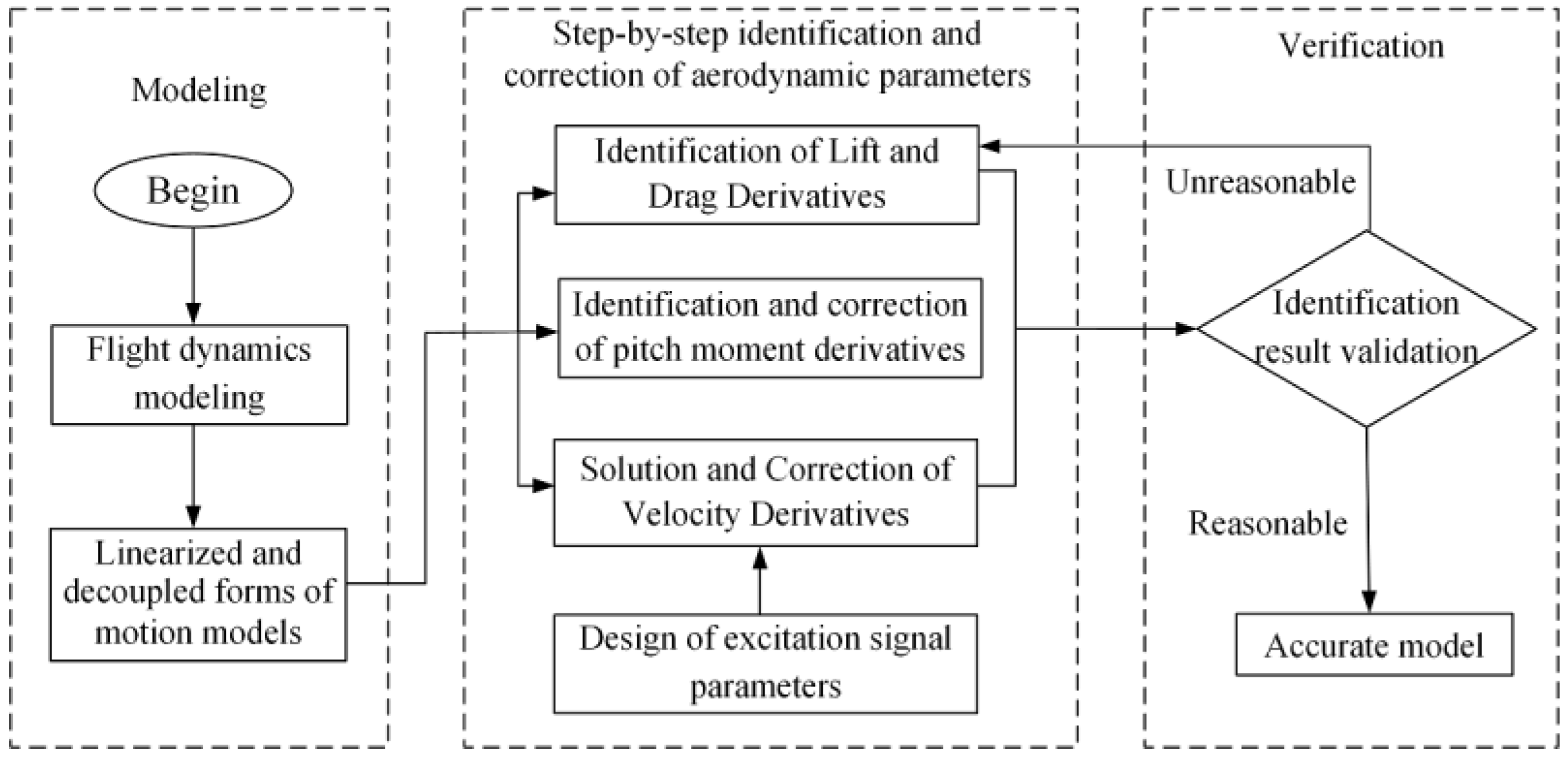
In summary, the longitudinal aerodynamic parameter identification method for BWB aircraft based on wind tunnel virtual flight tests is formed, and the specific steps are shown in Figure 4. First, the flight dynamics equations for the test model are established, and the equations of motion are linearized and decoupled to establish the identification model and analyze the difference in the longitudinal equations of motion between wind tunnel virtual flight and free flight. Second, we analyze the amplitude–frequency characteristics for the equations of motion and determine the frequency range and amplitude of the excitation signal. Third, according to the real-time measurement of the aerodynamic force of the aircraft through the strain gauge balance in the wind tunnel virtual flight test, the least squares method is used to complete the identification of lift and drag derivatives. Based on the motion of wind tunnel virtual flight, the maximum likelihood method is used to complete the identification of the pitch moment derivatives. The measured data of two groups of wind tunnel tests and the identified aerodynamic derivatives are used to calculate the velocity derivatives. Finally, the pitch moment derivatives are modified based on the difference between wind tunnel virtual flight and free flight, and the identification results are verified.

5. Verification of Wind Tunnel Virtual Flight Tests

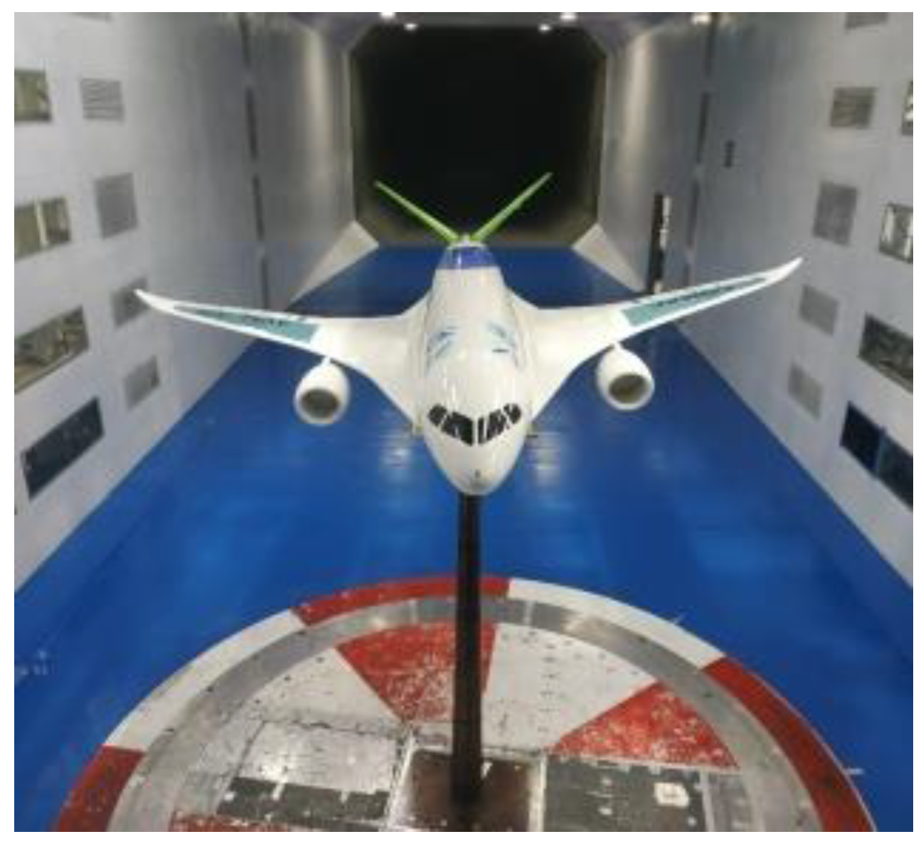
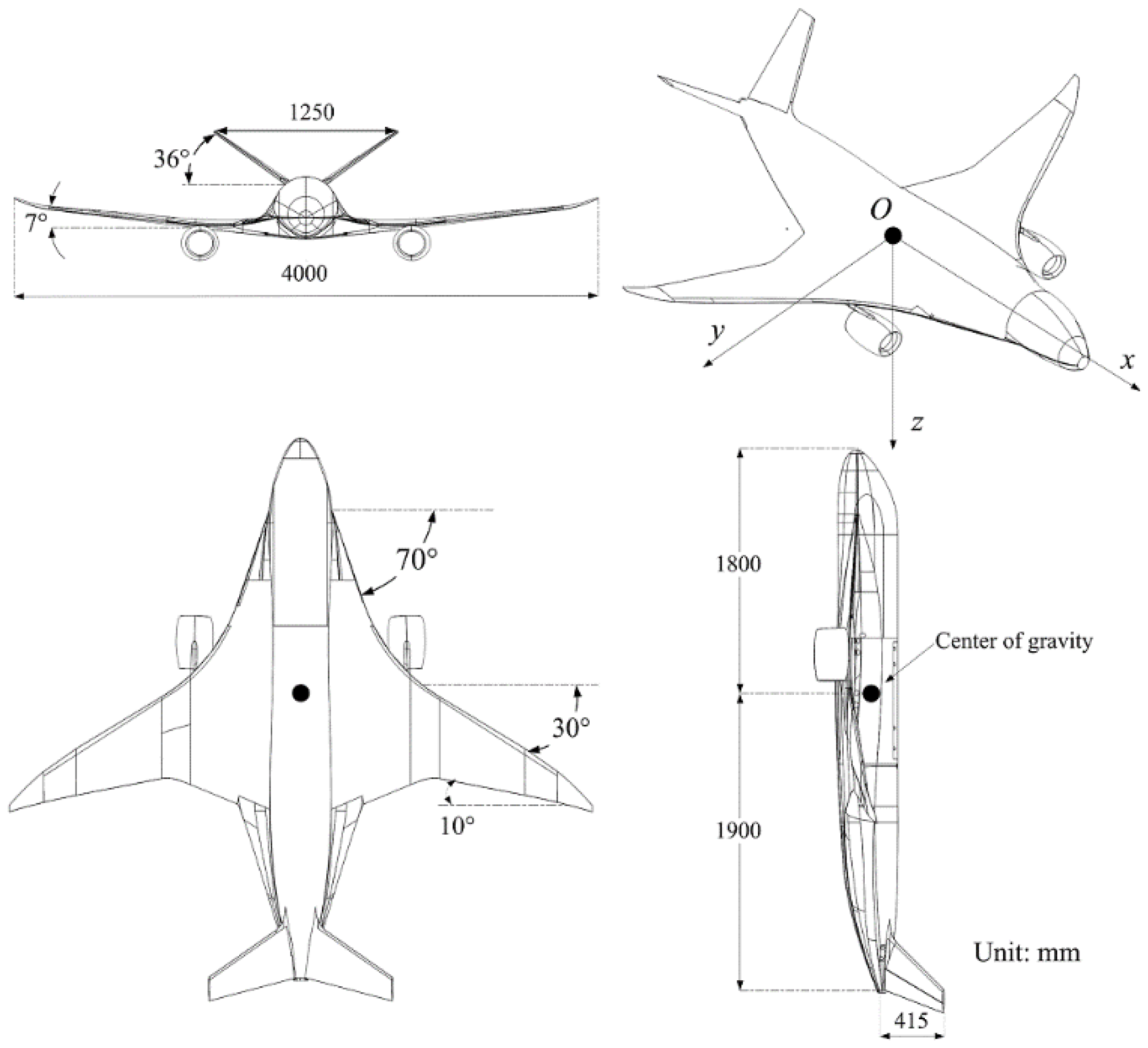
As shown in Figure 5, the test was carried out in the FL-10 low-speed wind tunnel closed test section of the AVIC Aerodynamics Research Institute. The cross-section size of the test section is 8 m × 6 m, the length is 20 m, and the maximum wind speed is 110 m/s. The model was installed in the wind tunnel by means of a belly support, and the scaling ratio of the test model is k = 1/9. The ontology design parameters of the scaled model can be obtained according to the similarity criterion [29,30], as shown in

Table 4. Ontology design parameters of the test model.

Parameters	Proportions	Full-Size Aircraft	Test Model
Wing span b (m)	1/9	36	4.00
Mean aerodynamic chord c (m)	1/9	1041	1.16
Wing area S (m2)	(1/9)2	241	2.98
Mass m (kg)	(1/9)3	49149	67.42
Pitch moment of inertia Iy (kg·m2)	(1/9)5	4044856	68.50
Yaw moment of inertia Iz (kg·m2)	(1/9)5	5166787	87.50
Roll moment of inertia Ix (kg·m2)	(1/9)5	1210504	20.50
Product of inertia Ixz (kg·m2)	(1/9)5	171242	2.90

and Figure 6.

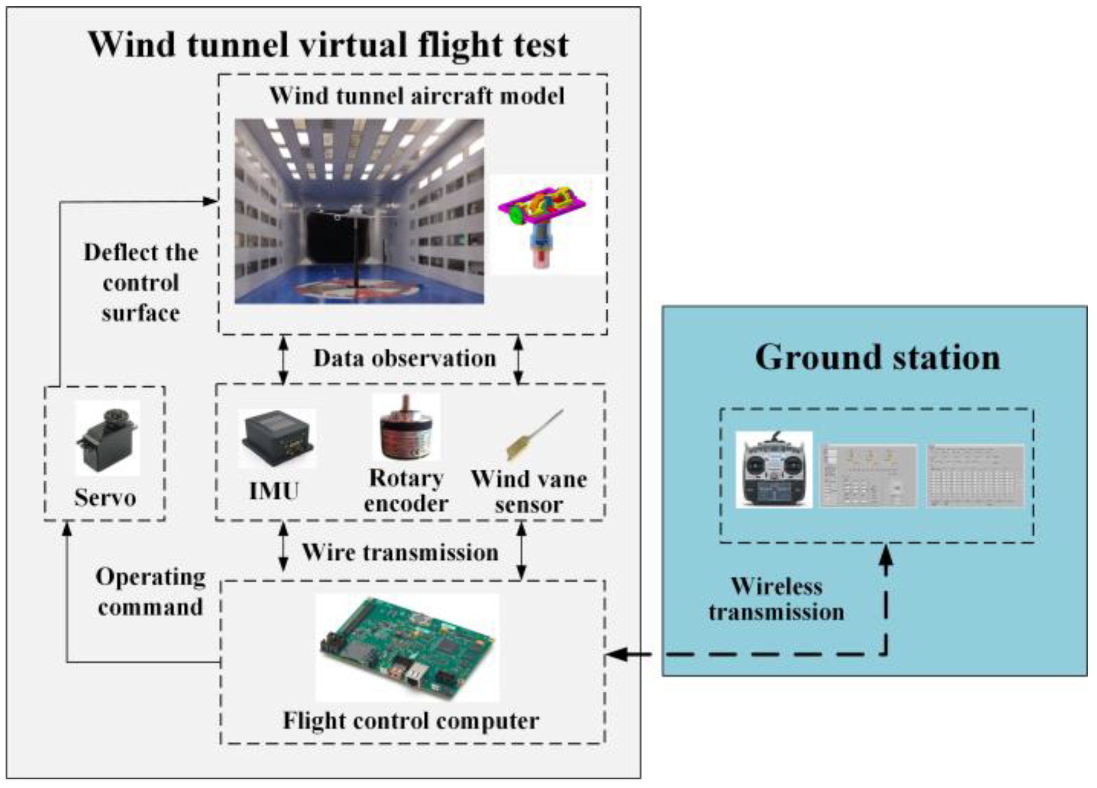
The flight test control and measurement system are shown in Figure 7. The scaled model is equipped with an attitude measurement sensor, a flight control computer, and servos that drive the deflection of the control surfaces. The attitude measurement sensor is used to measure the motion parameters of the aircraft; the flight control computer collects the sensor data, runs the control law algorithm, and controls the attitude of the scaled model through the control surfaces. The test control ground station can display the relevant data in the virtual flight test process in real time, including the angle of attack, sideslip angle, attitude angle, and angular velocity, as well as real-time information of the control surfaces. Meanwhile, the ground station can issue control commands based on the LabVIEW software platform.

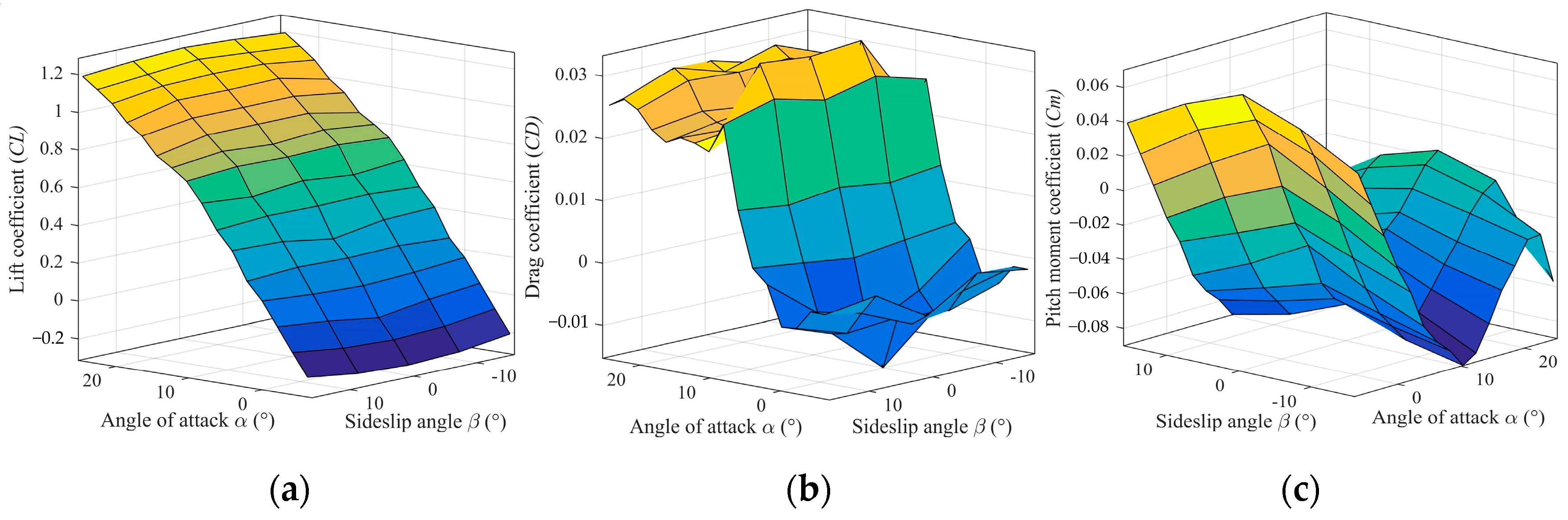
The wind speeds V = 30 m/s and α = 6° are selected as the trim flight state in the wind tunnel. Through the traditional wind tunnel force test on the test model, the aerodynamic database of the model at a speed of 30 m/s is obtained, as shown in Figure 8. In the traditional wind tunnel test carried out in this paper, the support interference correction test is carried out by the two-step mirror method, and the tunnel wall interference correction is carried out by the mirror analysis method [1].

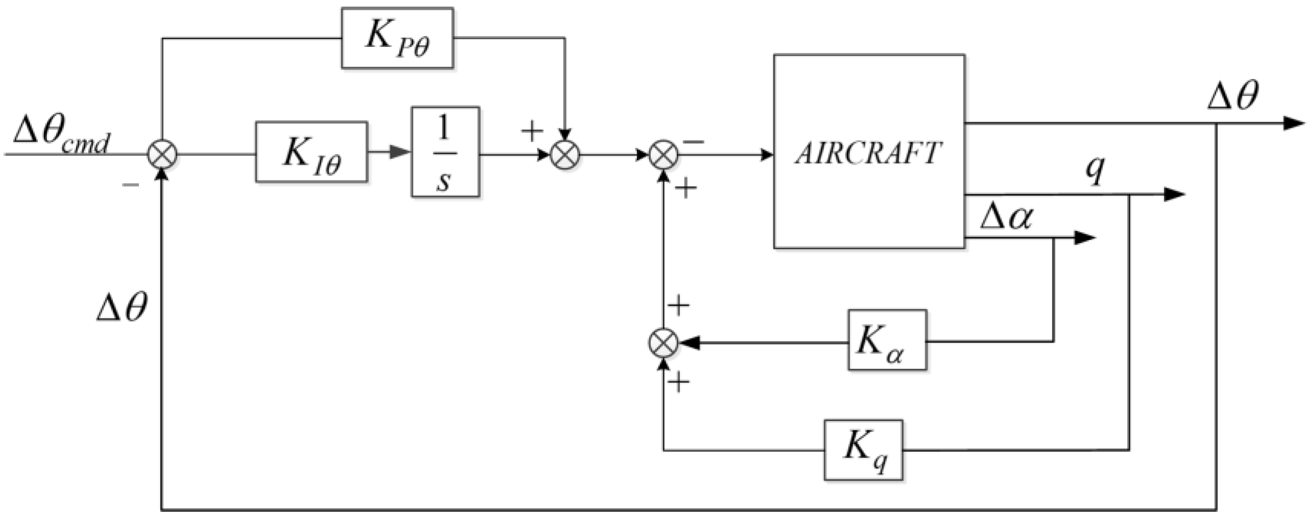
To precisely control the attitude angle of the model, a pitch angle control law structure is used in the longitudinal direction, as shown in Figure 9. The inner loop includes the angle of attack increment feedback K_α and pitch angle rate feedback K_q. The outer loop includes the pitch angle increment feedback Δθ. Among them, the incremental feedback of the angle of attack can increase the longitudinal static stability of the aircraft and improve the natural frequency of the short-period motion mode; pitch rate feedback is used to increase the damping of the aircraft’s pitch motion. The outer loop pitch angle increment is subtracted from the control command and passed through a PI link K_Pθ and K_Iθ to eliminate the error, thus enabling the model to track the pitch angle increment command. The longitudinal control law parameters of the test model are K_α = 1.6, K_q = 0.67, K_Pθ = 1.97, and K_Iθ = 0.9.

5.1. Design of the Excitation Signal

5.1.1. Determination of Frequency Ranges

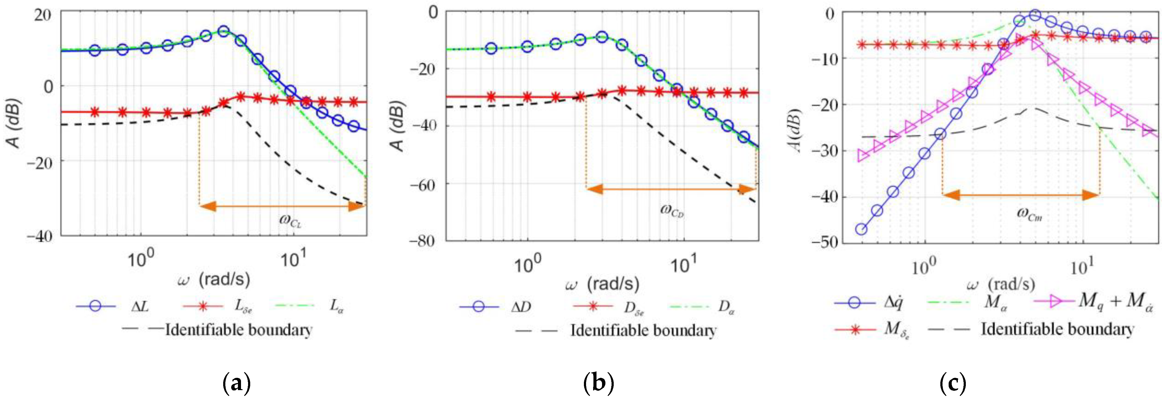
Based on the force measurement data from the traditional wind tunnel test shown in Figure 8, the longitudinal motion model shown in Equation (13) is established, and the amplitude–frequency response of the lift, drag, and pitch moment derivatives with the frequency of the excitation signal is drawn, as shown in Figure 10.

The pitch moment Bode diagram contains |M_α(ω)/δ_e|, |$M_q{+M}_{\dot{\alpha }}$(ω)/δ_e|, |M_δe(ω)/δ_e|, and |Δ$\dot{q}$(ω)/δ_e| curves, as shown in Figure 10a; the lift Bode diagram contains |L_α(ω)/δ_e|, |L_δe(ω)/δ_e|, and |ΔL(ω)/δ_e| curves, as shown in Figure 10b; and the drag Bode diagram contains |D_α(ω)/δ_e|, |D_δe(ω)/δ_e|, and |ΔD(ω)/δ_e| curves, as shown in Figure 10c. When the excitation signal frequency is too low, the response of the pitch rate q is almost zero, mainly in the form of a constant change in the aircraft’s angle of attack and altitude. Thus, the amplitude response of |$M_q{+M}_{\dot{\alpha }}$(ω)/δ_e| and |Δ$\dot{q}$(ω)/δ_e| in Figure 10 decreases, while the rest of the aerodynamic derivatives show little change in amplitude response. When the excitation signal frequency is too high, the aircraft response is much slower than the maneuvering speed, resulting in very little change in the aircraft’s angle of attack α and pitch rate q. As a result, the amplitude response of |M_α(ω)/δ_e|, |$M_q{+M}_{\dot{\alpha }}$(ω)/δ_e|, |D_α(ω)/δ_e|, |ΔD(ω)/δ_e|, |L_α(ω)/δ_e|, and |ΔL(ω)/δ_e| in Figure 10 decreases, while the amplitude response of the other aerodynamic derivatives does not change much. The short-period mode frequency of the aircraft at V = 30 m/s and α = 6° flight state is 4 rad/s, and the resonance peak of each curve in Figure 10 is approximately equal to the short-period mode frequency.

Based on the identifiability requirements of the aerodynamic derivatives introduced in Section 3, the identifiable boundaries of the pitch moment, lift, and drag derivatives are drawn and marked with dashed lines in Figure 10. To ensure the identifiability of each aerodynamic derivative, the amplitude response of all derivatives should be above the identifiable boundary. Therefore, the attention frequency range of the excitation signal determined by the pitch moment, lift, and drag derivative is determined as ${\omega }_{\mathit{Cm}}$= [1.3, 12.5] rad/s, ${\omega }_{\mathit{CL}}$ = [2.5, 25] rad/s, and ${\omega }_{\mathit{CD}}$ = [2.3, 25] rad/s, respectively. At the intersection of ${\omega }_{\mathit{Cm}}$, ${\omega }_{\mathit{CL}}$, and ${\omega }_{\mathit{CD}}$, the concerned frequency band of the longitudinal excitation signal is obtained, i.e., ω = ${\omega }_{\mathit{Cm}}$$\cap$${\omega }_{\mathit{CL}}$$\cap$${\omega }_{\mathit{CD}}$= [2.5, 12.5] rad/s, approximately between 0.5 and 3 times the short-period modal frequency.

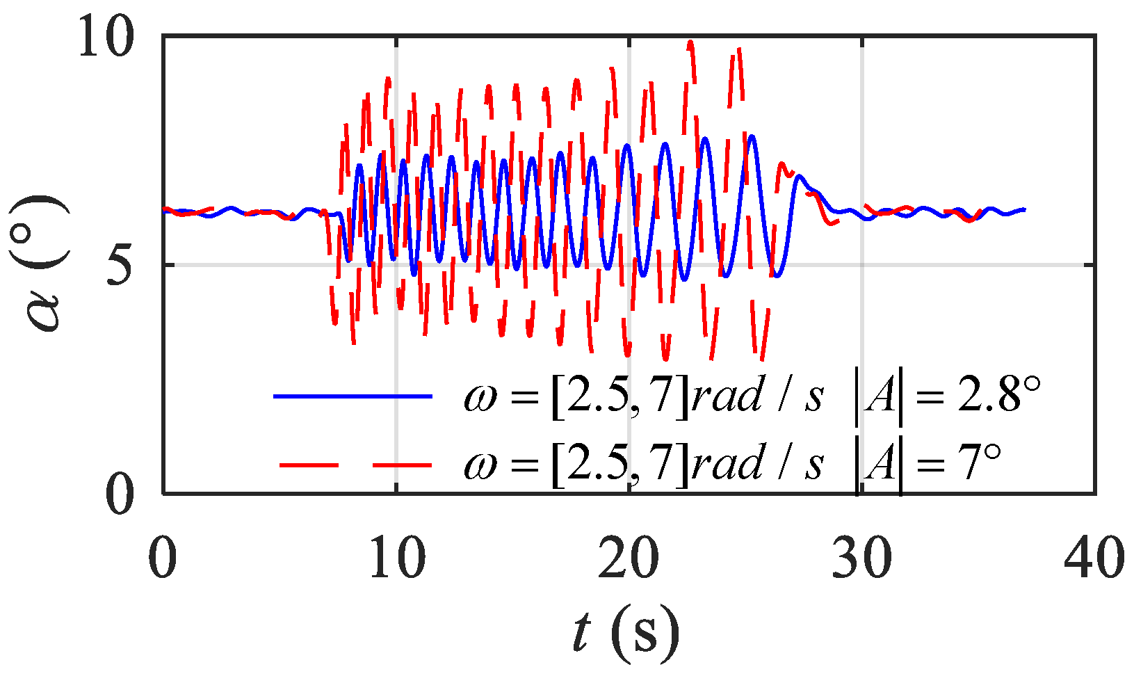
5.1.2. Determination of the Signal Amplitude

By selecting the appropriate excitation signal amplitude, the angle of attack changes in the range of ±2°. The frequency range of the excitation signal selected in this experiment is ω = [2.5, 7] rad/s. Frequency sweep signals with signal amplitudes of 2.8° and 7° are selected to act on the V-tail control surface, and the angle of attack response of the model is observed, as shown in Figure 11.

When the signal amplitude is 7°, the model angle of attack changes to 4°, and the range of the angle of attack changes greatly, which increases the error of the identification results. When the signal amplitude is 2.8°, the change in the model angle of attack is approximately 2°. Therefore, the amplitude of the excitation signal for this test is chosen as |A| = 2.8°. In summary, the model longitudinal excitation signal is a swept signal with frequency ω = [2.5, 7] rad/s and amplitude |A| = 2.8°.

5.2. Identification and Correction of Aerodynamic Derivatives

5.2.1. Identification of Lift and Drag Derivatives

The wind tunnel virtual flight test is carried out under the conditions of V₁ = 30 m/s, α₁ = 6°, and δ_e1 = −5.6°, and the outer ring of the control law is a 6° pitch angle command. The excitation signal acts directly on both sides of the V-tail control surfaces. The lift L_m and drag D_m of the test model are measured in real time by a strain gauge balance.

The lift L_m, drag D_m, angle of attack Δα, and deflection Δδ_e of the V-tail control surfaces measured in the test are substituted into Equation (16), and the lift and drag derivatives of the model can be directly identified by the least squares solution formula shown in Equation (18). The identification results are shown in the second column of

Table 5. Identification results of the aerodynamic parameters.

Parameters		Measured Values from Conventional Wind Tunnel	Identification Results	Corrected Identification Results
Lift and drag derivatives	$D_{*}$	52.18	50.36(3.49%) *	—
	Dα	694.26	640.03(7.81%)	—
	Dδe	26.62	22.96(13.75%)	—
	$L_{*}$	655.35	695.88(6.18%)	—
	Lα	5472.59	5235.02(4.34%)	—
	Lδe	316.84	290.65(8.26%)	—
Pitch moment derivatives	${\stackrel{\sim }{M}}_{\alpha }$	−5.68	−8.50(49.65%)	−5.56(2.11%)
	${\overline{M}}_q+{\overline{M}}_{\dot{\alpha }}$	−3.10	−3.17(2.26%)	—
	${\stackrel{\sim }{M}}_{\delta e}$	−13.95	−14.31(2.58%)	−13.92(0.21%)
Velocity derivatives	${\stackrel{\sim }{M}}_V$	0.019	0.002(89.47%)	0.021(10.52%)
	LV	43.47	40.55(6.71%)	—
	DV	3.64	3.36(7.69%)	—

* (): Deviation of identification results from conventional wind tunnel measurements.

, where the first column shows the aerodynamic derivatives measured in the conventional wind tunnel.

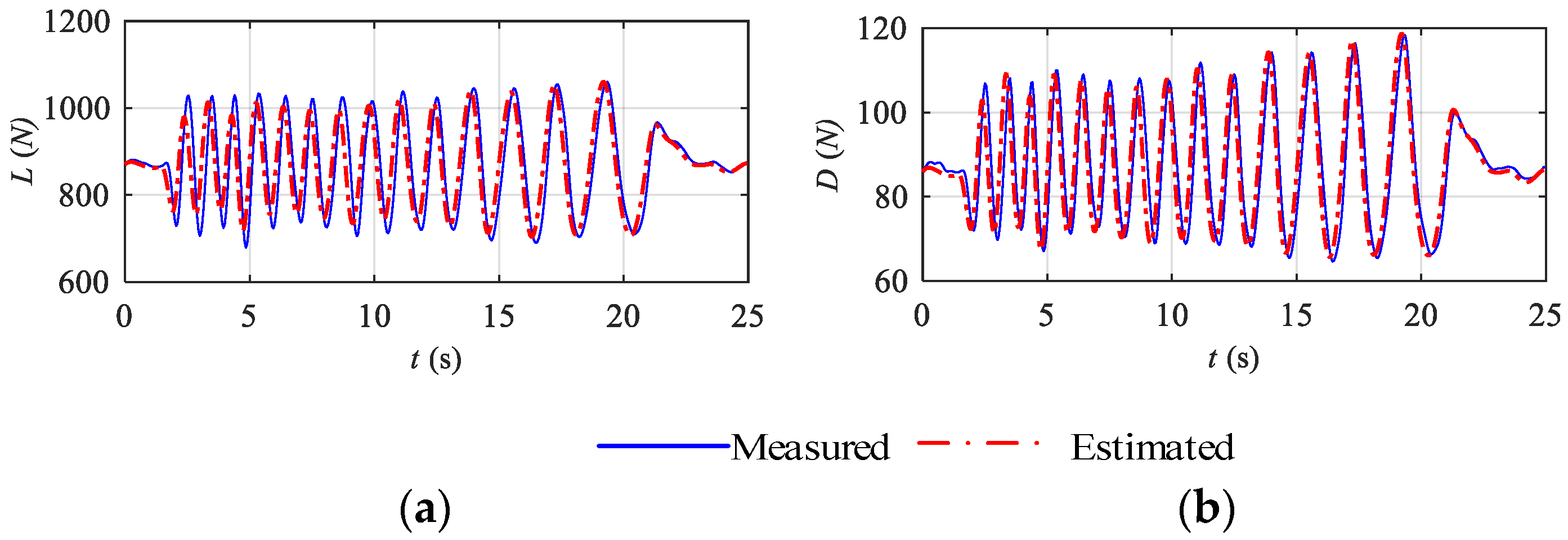
The identification results for the lift and drag derivatives are substituted into Equation (15) to establish the observation model of lift and drag in wind tunnel virtual flight test. The excitation signal used in the wind tunnel test is input into the identified model and compare the lift and drag simulation results with the data measured by the wind tunnel virtual flight test, as shown in Figure 12. The simulation data of the aerodynamic model are in high agreement with the data measured by the wind tunnel virtual flight test, and the maximum errors of the lift and drag curves are within 5%.

Comparison of the identification results with the conventional wind tunnel measurements in Table 5 indicates that the identification results of lift and drag derivatives are close to the conventional wind tunnel measurements. Because the strain gauge balance can directly measure the lift and drag of the model, the identification results are equal to the lift and drag derivatives in free flight, thus deviating less from the conventional wind tunnel measurements.

5.2.2. Identification and Correction of the Pitch Moment Derivatives

Under the same set of tests, the wind speed V_m, pitch angle θ_m, pitch rate q_m, V-tail control surface deflection δ_e, and angle of attack α_m of the model measured by the tests are substituted into Equation (21) as observations. The maximum likelihood method shown in Equations (22) and (23) is used to obtain the identification results of the pitch moment derivatives. The identification results are shown in the second column of Table 5.

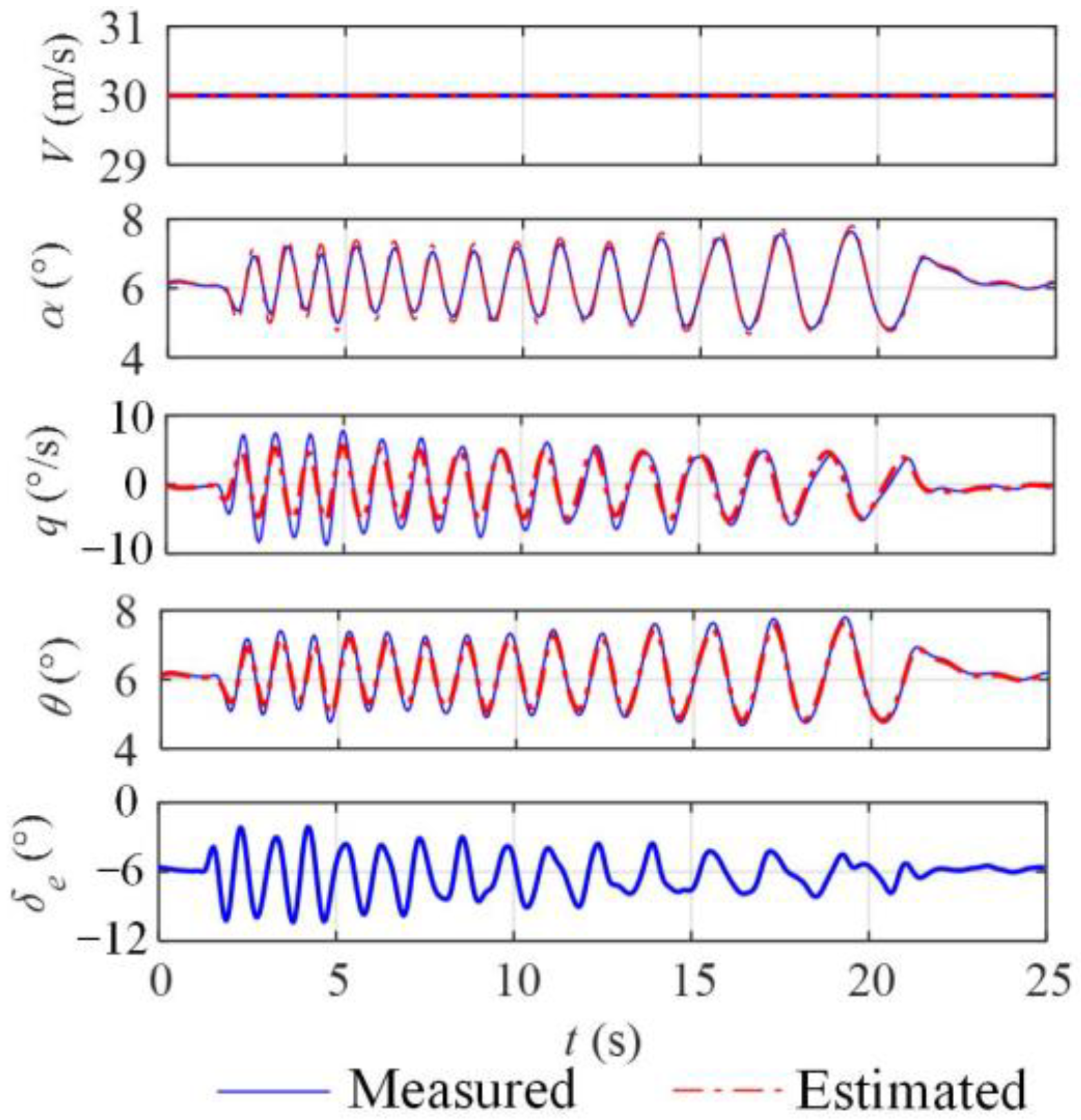
The identification results of pitch moment derivatives are substituted into Equation (19) to obtain the longitudinal motion model of the wind tunnel virtual flight test. The excitation signal used in the wind tunnel test is input into the identified model, and the simulation results of the identified model are compared with the test data, as shown in Figure 13. The response of the motion for the identified model is generally consistent with the wind tunnel virtual flight test data, which proves that the identified model can accurately simulate the longitudinal motion of the wind tunnel virtual flight test.

According to Table 5, there is a large deviation between the identification result of the pitch moment derivative ${\tilde{M}}_{\alpha }$ and the conventional wind tunnel measurement, and the identification results of ${\tilde{M}}_q$ + ${\tilde{M}}_{\dot{\alpha }}$ and ${\tilde{M}}_{\delta e}$ are approximately equal to the conventional wind tunnel measurements.

The reason for the deviation of the pitch moment derivatives identification results is that the equations of motion differ between the wind tunnel virtual flight and the free flight, so the pitch moment derivatives obtained from the wind tunnel virtual flight test are different from those of free flight. Equation (24) shows the relationship between the ${\tilde{M}}_{\alpha }$ and ${\tilde{M}}_{\delta e}$ in the wind tunnel virtual flight test and the derivatives ${\overline{M}}_{\alpha }$ and ${\overline{M}}_{\delta e}$ corresponding to the free flight. Using Equation (24), the derivatives of the free flight can be obtained by correcting the derivatives of the pitch moment obtained from the identification.

In Equation (24), ${\tilde{M}}_{\alpha }$, ${\tilde{M}}_{\dot{\alpha }}$, and ${\tilde{M}}_{\delta e}$ obtained from the identification are negative, and L_α and L_δe are positive, so the absolute values of the stability derivative ${\overline{M}}_{\alpha }$ and the maneuvering derivative ${\overline{M}}_{\delta e}$ in free flight are smaller than the values ${\tilde{M}}_{\alpha }$ and ${\tilde{M}}_{\delta e}$ obtained from the identification based on the wind tunnel virtual flight test.

According to Table 5, the values of L_α/m$V_{*}$, ${\tilde{M}}_{\alpha }$, and ${\tilde{M}}_{\dot{\alpha }}$ are on the same order of magnitude, so the difference between the identified ${\tilde{M}}_{\alpha }$ and the measured value of ${\overline{M}}_{\alpha }$ in the conventional wind tunnel is large. The value of L_δe/m$V_{*}$ is an order of magnitude lower than the values of ${\tilde{M}}_{\delta e}$ and ${\tilde{M}}_{\dot{\alpha }}$, so the difference between the identified ${\overline{M}}_{\delta e}$ and the wind tunnel measurement value ${\overline{M}}_{\delta e}$ is small.

According to Equation (24), the pitch moment derivatives ${\tilde{M}}_{\alpha }$ and ${\tilde{M}}_{\delta e}$ are corrected, and the correction results are shown in the third column of Table 5. The corrected pitch moment derivatives are approximately equal to the conventional wind tunnel measurements.

5.2.3. Solution and Correction of Velocity Derivatives

In another set of wind tunnel virtual flight test, the wind speed is adjusted to V₂ = 40 m/s. After the attitude angle of the model is stabilized, the angle of attack α₂ = 3°, V-tail control surface deflection δ_e2 = −2.7°, and lift and drag L₂ = 788 N and D₂ = 50.7 N of the aircraft are measured. The data of the two groups of wind tunnel virtual flight tests and the identification results of the first group of tests are substituted into Equation (26), and the velocity derivatives D_V, L_V, and ${\tilde{M}}_V$ are solved, as shown in the second column of Table 5.

Comparison of the velocity derivative solution results with the conventional wind tunnel measurements indicates that the velocity derivatives of lift and drag are approximately equal to the wind tunnel measurements, but the velocity derivative of pitch moment ${\tilde{M}}_V$ differs from the measured value ${\overline{M}}_V$ by an order of magnitude. The difference in pitch moment velocity derivatives arises from the difference in the equations of motion between wind tunnel virtual flight and free flight.

According to Equation (27), there is a difference between the derivative of ${\tilde{M}}_V$ in the wind tunnel virtual flight test and that of the free flight. The derivative of the pitch moment velocity ${\tilde{M}}_V$ can be corrected by using Equation (27) to obtain the derivative ${\overline{M}}_V$ of free flight.

In Equation (27), ${\tilde{M}}_{\dot{\alpha }}$ is negative and L_V and ${\tilde{M}}_V$ are positive, so the absolute value of the velocity derivative ${\overline{M}}_V$ in free flight is greater than the value ${\tilde{M}}_V$ obtained from the wind tunnel virtual flight test data. Since ${\tilde{M}}_{\dot{\alpha }}$ is an order of magnitude higher than ${\tilde{M}}_V$ and L_V/m$V_{*}$, the measured velocity derivative ${\overline{M}}_V$ is an order of magnitude higher than the solved velocity derivative ${\tilde{M}}_V$. The modified velocity derivative is shown in the third column of Table 5, and the modified velocity derivative is approximately equal to the conventional wind tunnel measurement.

5.3. Verification of Identification Results

The corrected aerodynamic derivatives in Table 5 are substituted into the A₁ and B₁ matrices in Equation (11) to construct the corrected longitudinal motion model for the wind tunnel virtual flight, as shown in Equation (28).

$$\left[\begin{array}{c}\dot{V}\\ \dot{\alpha }\\ \dot{q}\\ \dot{\theta }\end{array}\right]=\left[\begin{array}{cccc}-0.054& -0.58& 0& -9.8\\ -0.022& -2.73& 1& 0\\ 0.021& -5.68& -3.17& 0\\ 0& 0& 1& 0\end{array}\right]\left[\begin{array}{c}V\\ \alpha \\ q\\ \theta \end{array}\right]+\left[\begin{array}{c}-0.395\\ -0.157\\ -14.31\\ 0\end{array}\right]{\delta }_e$$

(28)

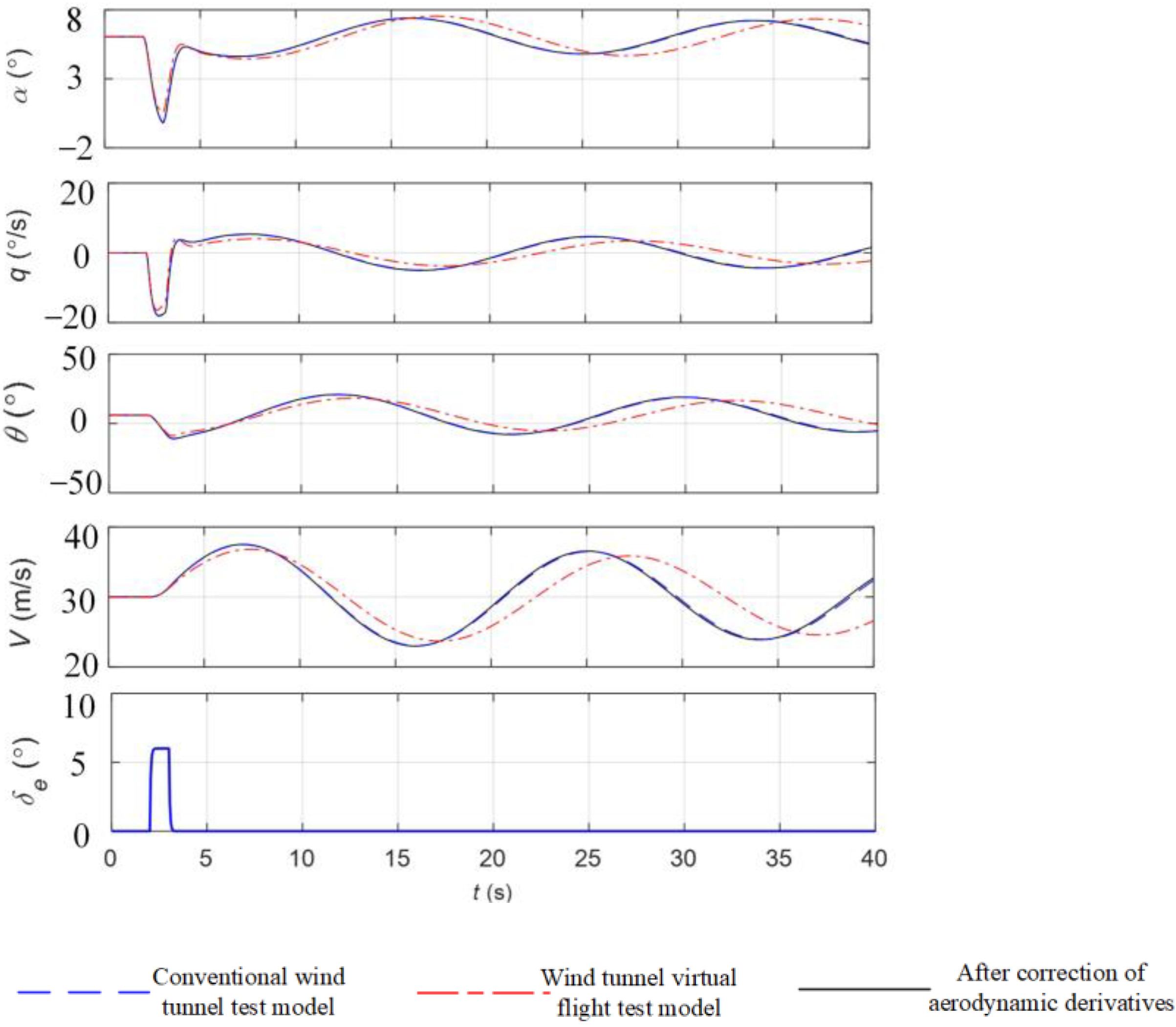
In addition, a mathematical simulation model of 6-DOF free flight is constructed based on the conventional wind tunnel force measurement data shown in Figure 8. The speed V₁ = 30 m/s, α₁ = 6°, and δ_e1 = −5.6° are chosen as the initial trim flight state for the mathematical simulation. A square wave signal is input to the V-tail control surface to make it deflect in the same direction, while the other control surfaces remain fixed. The results of comparing the simulation data of the longitudinal motion model of the wind tunnel virtual flight before and after the pitch moment derivative correction with the simulation data of the free flight are shown in Figure 14.

Based on a comparison between the motion response of the model before and after the correction of the aerodynamic derivatives with the motion of the free flight model, the goodness of fit (GOF) [31] of the two is shown in

Table 6. Goodness of fit of the wind tunnel virtual flight test with free flight.

GOF	V	α	q	θ
Before correction of aerodynamic derivatives	0.73	0.81	0.79	0.83
After correction of the aerodynamic derivatives	0.95	0.96	0.96	0.97

.

Figure 14 shows that the motion of the model identified based on the wind tunnel virtual flight test data differs significantly from the longitudinal motion of the free flight. The wind tunnel virtual flight motion response obtained after the aerodynamic derivative correction is in high agreement with the motion response of the free flight. The GOFs of each response variable of the wind tunnel virtual flight motion model are less than 0.85, while the GOFs of each response variable of the model after the correction are greater than 0.95.

In summary, compared with the wind tunnel virtual flight motion model obtained by direct identification, the motion of the model after the correction matches better with that of the free flight, indicating that the model after the correction can more accurately characterize the longitudinal motion of the aircraft in free flight.

6. Conclusions

(1)

In this article, longitudinal flight dynamics equations are derived for wind tunnel virtual flight tests. By linearizing the equations of motion to describe the wind tunnel virtual flight test as a decoupled form of the effects of free flight aerodynamic forces and support forces on the model motion, the differences between the longitudinal dynamics of wind tunnel virtual flight and free flight can be analyzed more intuitively, thus establishing a model for the identification of aerodynamic parameters.

(2)

To ensure the accuracy of identification for each aerodynamic derivative, a design method for the longitudinal excitation signals is proposed according to the analysis of the amplitude–frequency characteristics of the equation of motion, and the excitation signal frequency is approximately between 0.5 and 3 times the short-period modal frequency. A step-by-step identification method for the lift, drag, and pitch moment derivatives is established. A numerical solution method for the velocity derivatives that cannot be obtained through identification is introduced. Based on the differences in the equations of motion of the wind tunnel virtual flight and the free flight, a correction method for the identification result of the pitch moment derivatives is established.

(3)

The goodness of fit between the longitudinal motion model responses identified for the test data and the free flight is lower than 0.85, while the wind tunnel virtual flight test model after the correction can better simulate the longitudinal motion of the free flight, and the goodness of fit is higher than 0.95, thus verifying the accuracy of the method.

The proposed step-by-step identification and correction method of longitudinal aerodynamic parameters based on a wind tunnel virtual flight test is simple and the identification results are accurate. The aerodynamic parameters can be accurately identified at the early stage of aircraft design through the wind tunnel virtual flight test, and the results can be compared and modified with those of the traditional wind tunnel test. A video of the experiment can be found in Video S1 of the Supplementary Materials. In the future, we will propose a method for the identification of lateral-directional aerodynamic parameters based on wind tunnel virtual flight tests.