Abstract
Flapping-wing micro air vehicles (FWMAVs) have the capability of performing various flight modes like birds and insects. Therefore, it is necessary to understand the various flight modes of FWMAVs in order to fully utilize the capability of the vehicle. The unique flight modes of FWMAVs can be studied through the trajectory optimization. This paper proposes a trajectory optimization framework of an FWMAV. A high-fidelity simulation model is included in the framework to sufficiently consider the complicated dynamics of the FWMAV. The unsteady aerodynamics are modeled with the unsteady panel method (UPM) and the unsteady vortex-lattice method (UVLM). The effect of wing inertia is also considered in the simulation model. In this study, transition flight trajectories are searched with the proposed framework. An optimal control problem is formulated for the transition flight from hovering to forward flight and transcribed to the parameter optimization problem with the direct shooting method. The cost function is defined as energy consumption. The same converged solution can be obtained with different initial guesses. The optimization results show that the FWMAV utilizes the pitch-up maneuver to increase altitude, although the forward speed is reduced. This pitch-up maneuver is performed more actively when the target velocity of transition is low, or the wind condition is favorable to acceleration.
1. Introduction
Flapping-wing micro air vehicles (FWMAVs) have been developed to pursue the high flight performance of birds and insects. Especially, the insect-like FWMAVs have a wider range of applications because of their various flight modes and ability to freely transit each flight mode. To fully utilize the flight ability of FWMAVs, optimization studies have been conducted. Many studies have focused on the wing kinematics optimization during hovering [1,2,3,4], forward [5], and ascending [6] flights. FWMAVs can perform more various flight modes like the transition flight and dynamic soaring as well as the hovering, forward, and ascending flights. Therefore, these unique and advantageous flight modes of FWMAVs require an in-depth study.
Trajectory optimization is a technique used to find the open-loop solution for an optimal control problem [7]. The solution of trajectory optimization is the sequence of inputs to minimize the cost function while satisfying the constraints. One main advantage of trajectory optimization is the ability to handle the constraints. Therefore, feasible wing kinematics can be obtained with the constraint of inputs. Thus, the trajectory optimization is one of the best ways to study the feasible flight trajectory of FWMAVs. The sequence of inputs can be directly applied as open-loop control. In addition, guidance and control laws, which can be applied to the general situation with modeling uncertainty and disturbance, can be designed based on the optimization results. Meanwhile, the selection of the modeling method is important in the trajectory optimization of FWMAVs. The fidelity of the model must be considered because the error from the modeling cannot be canceled by a feedback loop when the open-loop solution is applied. In addition, the computational cost of the model should be considered because numerous simulations are required in the optimization process.
The insect flight is highly characterized by unsteady and complicated aerodynamics at low Reynolds number [8,9,10]. To estimate the aerodynamic load, computational fluid dynamics (CFD) and quasi-steady (QS) aerodynamic model have been commonly used [11,12,13]. CFD is a high-fidelity approach that can give a precise prediction of the complex flow fields of a flapping-wing. However, CFD requires significant computational time, making it unsuitable for optimization problems. QS model is a low computational cost model with low fidelity. Especially, some of the aerodynamic coefficients in the QS model are obtained by experiment or CFD [14,15]. Therefore, the accuracy is dependent on the used conditions in experiment or CFD, such as wing geometry, kinematics, forward speed and so on. When this QS model is applied to different condition, the accuracy could be decreased. Therefore, the QS model has a limitation in a trajectory optimization process searching the unknown trajectories.
A few studies have been conducted on trajectory optimization for FWMAVs [16,17]. Hussein et al. [16] conducted the trajectory optimization for the transition flight from forward flight to hovering. The cost was defined as the traveled distance during the transition. The optimal trajectory included a rapid pitch-up maneuver with speed decline. Dietl and Garcia [17] also performed trajectory optimization for the transition flight from hovering to forward flight. The searched input had a bang-bang nature due to the minimum time control problem with upper and lower bounds on the controllers. As the forward flight speed increased, more time was required for the transition. It is noteworthy that both studies used the QS model as the aerodynamic model and ignored the effect of wing inertia. The wing inertia has been commonly neglected in the control-oriented model [18,19,20], which is used to design the feedback controller. However, neglecting the wing inertia has a significant effect from a simulation standpoint [21].
Although the above-mentioned research works have been conducted on the trajectory optimization of FWMAVs, the simplified modeling used in the previous research cannot consider complex aerodynamic effects and wing inertia. Therefore, the trajectory of their research does not fully use the flight capabilities of FWMAVs, and this necessitates the optimization of the FWMAV trajectory with the higher fidelity simulation model.
In this study, a new trajectory optimization framework for FMWAVs is proposed in terms of a simulation model with a higher fidelity. The simulation model in the framework uses the UVLM and the UPM to compute the aerodynamic force. The unsteady vortex-lattice method (UVLM) and unsteady panel method (UPM) are the potential-based aerodynamic model. These methods are computationally less expensive than CFD, while they can consider the unsteady effects like the wake effect; it is one of the main aerodynamic characteristics of the FWMAV, but it cannot be considered using the QS model. Especially, this wake effect should be considered for the transition flight because the advance ratio, which affects the wake effect, is varying with the accelerated forward velocity. The wing inertia effect is also considered in the simulation model.
Optimization variables are defined, considering the increased computational burden by the higher fidelity model. The optimal control problem is formulated for an insect-like FWMAV to conduct an efficient transition flight from hovering to forward flight, and the cost function is defined as energy consumption. The formulated optimal control problem can be solved with two categories of methods: indirect methods and direct methods. Indirect methods introduce the Lagrange multipliers and construct the necessary conditions for optimality. Then, the solution satisfying the conditions is searched. On the other hand, the direct methods represent the control variables and/or the state variables with discretized optimization variables. Then, the problem is converted to the parameter optimization problem and can be solved by any parameter optimization solver. The direct method is used in this study because it has a wider convergence region and does not require the initial guess for the costate variables.
2. Materials and Methods
2.1. FWMAV Model and Kinematics
In this paper, the natural flier, hawkmoth, is the reference insect and has been generally used in research on insect-like FWMAVs [22,23,24]. The wing is assumed to be rigid and connected with a three degree-of-freedom (3 DOF) revolute joint to the body. The hawkmoth parameters presented in Table 1 are based on the measurements by Ellington [25] and R. O’hara and A. Palazotto [26]. In Table 1, , and are the mass, radius, and mean chord length of the wing, respectively. and are the mass and length of the body. is the distance from the center of mass of the body to the tip of the head, and is the distance from the center of mass to the wing-base pivot. Figure 1 shows the FWMAV and geometry parameters of the body.

Table 1.
Geometry and mass parameters of the reference insect.
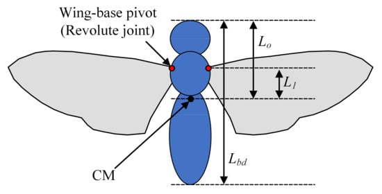
Figure 1.
FWMAV and parameters of the body.
Figure 2 shows reference frames and angles to define the kinematics of the FWMAV. The body-fixed frame is attached to the center of the mass of the body, and the ground-fixed frame is the inertial frame. The wing-fixed frame is attached to the wing-base pivot where the axis is parallel to the spanwise direction, and the axis is parallel to the chord direction. Stroke plane frame is used to define the wing kinematics. The axis is parallel to the axis, and the axis makes an angle of and with respect to the and planes, respectively.
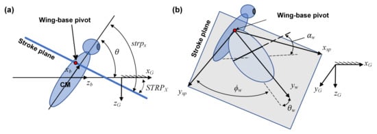
Figure 2.
Reference frames and positional angle in (a) side view and (b) isometric view.
The orientation of the wing is defined by three Euler angles on the stroke plane. The sequence of the rotation should be 3-1-2 corresponding to the sweep angle , the elevation angle , and the rotation angle . The wing kinematics of the FWMAV is defined by the 3-order Fourier series as:
where is the flapping frequency. and are the Fourier coefficients determined by fitting the measurement data [27], and prescripts , , and denote that the Fourier coefficients are for the sweep, elevation, and rotation angle, respectively. Here, the wing kinematics is assumed to be symmetrical by the plane.
2.2. Simulation Environment
Figure 3 shows the developed simulation environment, which consists of the three parts: aerodynamic model, multibody dynamics solver, and controller. The equation of motion is time-integrated by the multibody dynamics solver. The sub-routine, which is programmed in the FOTRAN language, computes the aerodynamic load on the FWMAV. The wing kinematics of FWMAV depends on the control variables, and the control variables are computed by a controller, which will be designed in Section 2.4.
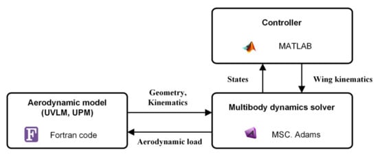
Figure 3.
Simulation environment.
2.2.1. Aerodynamic Model
The unsteady panel method (UPM) and the extended unsteady vortex-lattice method (UVLM) are used to compute the aerodynamic forces. Both methods are based on the potential flow theory [28] with the assumption that the flow is assumed to be incompressible, inviscid, and irrotational.
For the potential flow, the velocity potential needs to satisfy a Laplace equation:
The velocity potential also needs to satisfy three boundary conditions, including the far field, the Neumann, and the Dirichlet boundary conditions, as in Equations (5)–(7), respectively.
Here, and are the position vector, the velocity of the body, the normal vector of the body surface, and the velocity potential of the inside of the body, respectively. The solution of can be expressed by the sum of source and doublet distribution on the body and wing surface [28].
The UPM is applied to the bluff object like body. The body surface is discretized into the triangular and quadrilateral panels, and each panel has a constant-strength source and doublet. The UVLM is applied to the thin object like a wing. The UVLM can be considered as a reduced version of the UPM. The source strengths on upper and lower surfaces cancel each other. The doublet elements on upper and lower surfaces are equivalent to the vortex ring [28]. The UVLM is extended by applying the leading-edge suction analogy model to consider the effect of spiral leading-edge vortices. The vortex-core growth model is used to incorporate the effect of eddy viscosity in the vortex wake and tackle the singularity problems. The other viscosity effects cannot be considered in the used aerodynamic model because the flow is assumed to be inviscid. However, viscosity effects do not have a significant contribution to the aerodynamics of insects [29]. Therefore, ignoring other viscosity effects is reasonable considering the reduced computational time compared to higher fidelity models, such as CFD. More details about the aerodynamic model are found in the study by Nguyen et al. [30,31].
2.2.2. Multibody Dynamics Solver
The nonlinear equations of motion are established and solved based on the multibody dynamics solver, MSC. Adams. Such multibody dynamics solvers have been used to study dynamics and control of FWMAVs [32,33,34]. The aerodynamic force and moment required in the solver are computed with the UPM and the extended UVLM.
In the MSC. Adams, the equations of the motion are formulated as a set of nonlinear differential-algebraic equations (DAE) presented as:
where is the vector containing the coordinates that represent displacement, represents the mass matrix of the system, represents the kinematic constraints, contains the Lagrange multipliers for the constraints, is the vector containing applied forces and gyroscopic terms of the inertia forces, represents the matrix that projects in direction, and represents the gradient of the constraints.
2.3. Trim Search
A trim condition is needed to formulate an optimal control problem and design a pitch controller. Finding the trim condition is complicated because of the oscillating aerodynamic load within a wingbeat stroke. In this study, the trim search algorithm proposed by Kim et al. [35] is used. During the trim search process, the flapping frequency, the mean sweep angle, the mean rotation angle, and the initial value of states are searched to satisfy the trim criteria as presented in Equations (10)–(12).
Here, the subscript means that the value is represented in the ground-fixed frame. The upper bar denotes the wingbeat-cycle-averaged value. The trim of the FWMAV is obtained about the cycle-averaged states due to the oscillating characteristic of the system. is applied force, is applied moment, and is 6-DOF states. and are the velocity components along the and axes, respectively. and are the angular velocities about the and axes, respectively. means given forward flight velocity. Figure 4 shows the flowchart of the trim search algorithm.
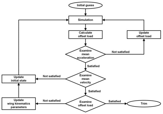
Figure 4.
Flowchart of a trim search algorithm.
After searching the trim, the equations of motion can be linearized at each trim condition. The eigenvalues of the system matrix are compared with those of Nguyen et al. [30], who used the same aerodynamic model. Figure 5 shows that the eigenvalues of longitudinal dynamics are similar to each other. The states of the longitudinal dynamics are the velocity components along the and axes, the angular velocity about the axis, and the pitch angle of the body. The power consumption for the trim flights is also calculated (Figure 6), where the calculation for the power consumption will be presented in Section 2.4.2.
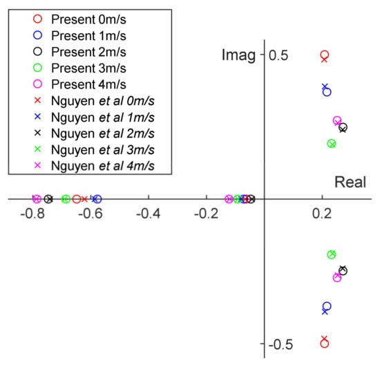
Figure 5.
Eigenvalues comparison of the longitudinal dynamics from the present model and Nguyen et al. [30].
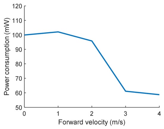
Figure 6.
Cycle-average power consumption of the trim flight.
2.4. Optimal Control Problem Formulation
In this section, an optimal control problem is formulated for the FWMAV to conduct transition flight from hovering to the forward flight with a target velocity. Since the reference insect, hawkmoth, can fly up to 5 m/s [36], the target velocities of the transition flight are set as 2, 3, and 4 m/s in the range. In addition to accelerating to the target velocities, there should be no altitude loss because the FWMAV consumed additional energy to recover the altitude loss after the transition. In this section, the control variables, cost function, and constraints of the optimal control problem are defined.
2.4.1. Control Variables
More control variables lead to a more complex optimization problem. Therefore, some appropriate wing kinematics parameters should be defined as the control variables, and the other parameters need to be fixed or defined as a function of state and control variables. In this paper, two control variables are used: flapping frequency and sweeping bias . The flapping frequency mainly affects the magnitude of the aerodynamic force [37] while the sweeping bias is used to control the pitch axis. The two control variables have been commonly used in the control of FWMAVs [38,39,40]. The two control variables determine the wing kinematics as:
where and are functions of the forward velocity determined by interpolation between the values obtained by the trim search.
needs to be frequently changed in order to stabilize the FWMAV, which requires many nodes for the transcription method. Even though the used aerodynamic model is more computationally efficient than CFD, it is not as fast as the QS model. Therefore, too many nodes need to be avoided because more nodes require more time for optimization. The pitch controller is designed to reduce the number of nodes. is determined by the pitch controller as follows:
Here, the gains and were respectively determined as −0.08, −0.74, and −5.14 by trial and error to maximize the pitch command tracking performance of the FWMAV. Eventually, the pitch command of the controller and flapping frequency become inputs of the total system, which includes the system dynamics and the pitch controller. The inputs ( and ) are the optimization variables, which are obtained from the optimization.
2.4.2. Cost Function
The cost function is defined as the mechanical energy consumption for the transition flight as follows:
where
In this paper, it is assumed that the FWMAV does not store the energy in the elastic elements during a period of negative work like the reference insect [41]. The final transition time is given as 2 s.
2.4.3. Constraints
For the complete transition flight, the final forward velocity should be higher than the target velocity. The direction of the vertical velocity should not be downward, and the altitude should not decrease. In addition, the initial states are set to be the values of hovering obtained by the trim search. Equations (21)–(24) show the constraints on states. The initial and final inputs are set to be the inputs of hovering and forward flight with the target velocity, respectively. Equations (25)–(28) show the constraints on inputs.
Here, is the longitudinal state vector . As mentioned earlier, is set as 2, 3, and 4 m/s. is the tolerance for the velocity constraints, which is set to be 0.3 m/s.
Equations (29)–(32) show the other constraints on inputs where is the flapping period during hovering flight. These constraints on the inputs and the rates of the input are for the feasible flapping kinematics. It can also prevent the numerical simulation from diverging. The input ranges are set not to be more than twice the range of the measurement values of the real hawkmoth [27]. The bound on the inputs rates are set so that more than 10 cycles of flapping are required to change the inputs from the upper and the lower bound or vice versa.
2.5. Transcription and Parameter Optimization Problem
The formulated optimal control problem is transcribed to the parameter optimization problem. Here, the used transcription method is the direct shooting method. The advantage of this technique is that there are fewer optimization variables because only the inputs, not the states, become the optimization variables to be searched.
With the direct shooting method, each input is discretized into a set of nodes. Continuous inputs are obtained by the linear interpolation of the discretized input and then used in the simulation to calculate the cost and constraints. Now, the optimal control problem is transcribed to the parameter optimization problem by searching a limited number of variables. The parameter optimization problem is solved using FMINCON, a MATLAB solver, and the sequential quadratic programming (SQP) is used as an algorithm of the solver.
3. Results and Discussions
The SQP is the gradient-based method requiring an initial guess, and the main concern of the method is that it can be sensitive to the initial guess. Therefore, the effect of the initial guess is investigated. After that, the optimization results are introduced then followed by the optimization results in the presence of the wind.
3.1. Initial Guess for SQP
If the optimized results are changed with the initial guess, the results are likely to be a local minimum. On the other hand, if the optimized results are not changed with the initial guess, the results have a high probability of becoming a global minimum, and the problem is not sensitive to the initial guess. In order to check how sensitive the formulated problem is to the initial values, optimization is performed with three different initial guesses in the case of = 3 m/s.
Figure 7 shows the used initial guesses. The guess #1 is shaped like a ramp function, and the guess #2 is given by linear interpolation between the initial and final input constraints as presented in Equations (25)–(28). The guess #3 has an arbitrary shape. Figure 8 shows that the results with the three initial guesses are the same as each other. This shows that the formulated problem can be considered not to be sensitive to the initial guess. The linear interpolated guess will be used in this study.
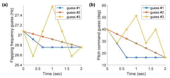
Figure 7.
Three different initial guesses for SQP: (a) flapping frequency; (b) pitch command.
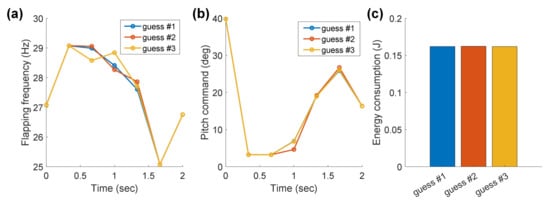
Figure 8.
Optimized (a) flapping frequency, (b) pitch command, and (c) energy consumption with the three different initial guesses.
3.2. Optimization Results
With 7 nodes (See Appendix A for a discussion of the node number) and a linear interpolated initial guess, the optimization is conducted for the transition flight with the three target velocities. The optimization converges to the feasible solution except in the case of = 4 m/s. To obtain a feasible solution for this case, the frequency range or the final time can be increased. The result with twice the frequency range (±4 Hz) is used in the comparison analysis with the same time duration.
Figure 9 shows the optimization results of the flapping frequency and pitch command. A higher target velocity leads to an overall higher flapping frequency and energy consumption. For all cases, the pitch command decreases to the lower bound in the initial stage, and then a pitch-up maneuver is conducted. In Figure 10c, all of the transition flights are completed without the additional increase in altitude. The cases of = 2 and 3 m/s have similar trajectories, which are characterized by a down-up shape, while the trajectory of = 4 m/s is slightly different. Because the given time is not enough to accelerate to 4 m/s, an overall high flapping frequency is maintained for acceleration and leads to more lift, which eliminates the altitude loss. In order to observe how the trajectory changes for a sufficient time like 4 s, an additional optimization is conducted. As shown in Figure 11c, the down-up trajectory can be obtained like in the cases of = 2 and 3 m/s.
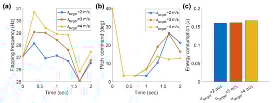
Figure 9.
Optimized (a) flapping frequency, (b) pitch command, and (c) energy consumption.
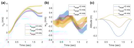
Figure 10.
(a) Forward velocity, (b) vertical velocity, and (c) altitude of optimal trajectory.
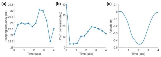
Figure 11.
(a) Forward velocity, (b) vertical velocity, and (c) altitude of the optimal trajectory ( = 4 m/s and = 4 s).
In Figure 9b, the low pitch command is necessary in the initial stage for the rapid acceleration even though this maneuver causes altitude loss, as seen in Figure 10c. After low pitch command, for = 2 and 3 m/s, the pitch command goes beyond the trim pitch angle of the target velocity, which is set by Equation (28). Although the pitch-up maneuver decreases the forward velocity (Figure 10a), the maneuver helps FWMAVs to gain much altitude (Figure 10c). Considering the low flapping frequency during the ascending, the pitch maneuver has a greater effect on the altitude gain than the frequency. Therefore, these optimal trajectories can be understood as conducting additional acceleration over the target velocity and utilizing the extra forward velocity to gain potential energy through a pitch-up maneuver. This pitch-up maneuver is actively performed in the low-velocity transition where enough forward velocity can be sacrificed to increase the altitude.
3.3. Wind Effect
The wind can affect the trajectories of natural fliers. Birds are known to perform the dynamic soaring to utilize the wind. Therefore, it is necessary to consider the wind effect in the trajectory optimization framework. In this section, additional optimization in the presence of the wind is conducted for the 3 m/s transition. Four wind direction namely headwind, tailwind, updraft, and downdraft, are considered, and their wind speed is given as 0.3 m/s.
The optimization converges to the feasible solution except for the downdraft. For the downdraft, a feasible solution can be obtained after the frequency range increased to ±4 Hz. Figure 12 and Figure 13 show the optimized result for the different wind directions. In Figure 12b, the highest pitch-up maneuver is observed for the tailwind. The reason is that the tailwind is favorable to the acceleration, and this can be used to gain altitude via pitch-up maneuver. This maneuver results in the largest altitude change, as shown in Figure 13. On the other hand, the pitch-up maneuver is the lowest in the presence of the headwind, which is not favorable to acceleration. In Figure 12a, the flapping frequency for the downdraft and updraft is distinctively different from other wind conditions. A lower flapping frequency is maintained to save energy in the presence of the updraft, while a higher flapping frequency is needed to satisfy the altitude constraint for the downdraft. Figure 12c shows that the vertical direction of the wind mainly affects the energy consumption of the transition flight. In addition, headwind and updraft decrease the energy consumption compared to the no wind condition.
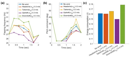
Figure 12.
Optimized (a) flapping frequency, (b) pitch command, and (c) energy consumption in the presence of different wind directions.
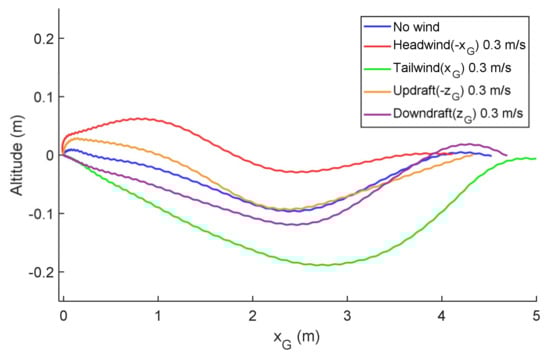
Figure 13.
Flight trajectories for different wind directions.
4. Conclusions
In this paper, the trajectory optimization framework was proposed, and an efficient transition flight trajectory of the FWMAV was obtained. The multibody dynamics solver, extended UVLM, and UPM were used to ensure the feasibility of the open-loop solution, which is dependent on the fidelity of the simulation model. The optimal control problem was formulated as the minimum energy transition flight without altitude loss. To reduce the optimization time of the computationally expensive simulation model, the number of nodes was reduced using the pitch controller. As a result, the pitch command and flapping frequency were defined as the optimization variables. The formulated optimal control problem was transcribed to the parameter optimization problem with the direct shooting method, and the parameter optimization problem was solved with SQP.
The optimization results with three different initial guesses were similar, showing the reliability of the optimized solution and that the formulated problem is not sensitive to the initial guess.
The energy-optimal trajectory for the transition flight was investigated. The results can be summarized as follows:
- (1)
- When the target velocity is low (2 and 3 m/s), the FWMAV performs additional acceleration over the target velocity. After that, the FWMAV sacrifice the forward energy to gain the potential energy via pitch-up maneuver.
- (2)
- The pitch-up maneuver is performed more actively when the condition is favorable to acceleration: the target velocity is low, or the wind direction is tailwind.
- (3)
- When the wind direction is up and downward, the flapping frequency and energy consumption are distinctively different from the other wind conditions.
The endurance of a FWMAV is expected to be increased by the proposed framework and the trajectory which can be obtained using the framework. Moreover, the proposed trajectory optimization framework, and the developed simulation environment can be used to design the closed-loop guidance and control law, which can be more generally applied.
Author Contributions
Conceptualization, S.-G.L., H.-H.Y. and R.A.-A.; methodology, S.-G.L. and H.-H.Y.; software, S.-G.L.; validation, S.-G.L.; formal analysis, S.-G.L. and H.-H.Y.; investigation, S.-G.L., H.-H.Y. and R.A.-A.; resources, J.-H.H.; writing—original draft preparation, S.-G.L.; writing—review and editing, S.-G.L., R.A.-A. and J.-H.H.; visualization, S.-G.L.; supervision, J.-H.H.; project administration, J.-H.H.; funding acquisition, J.-H.H. All authors have read and agreed to the published version of the manuscript.
Funding
This research was supported by Unmanned Vehicles Core Technology Research and Development Program through the National Research Foundation of Korea (NRF) and Unmanned Vehicle Advanced Research Center (UVARC) funded by the Ministry of Science and ICT, the Republic of Korea (2020M3C1C1A01083415).
Institutional Review Board Statement
Not applicable.
Informed Consent Statement
Not applicable.
Data Availability Statement
Not applicable.
Conflicts of Interest
The authors declare no conflict of interest.
Nomenclature
| Fourier coefficients for the wing kinematics, | |
| mean chord length of the wing, | |
| applied force vector, | |
| flapping frequency, | |
| distance from the center of mass of the body to the tip of the head, | |
| distance from the center of mass to the wing-base pivot, | |
| length of the body, | |
| applied moment vector, | |
| mass of the body, | |
| mass of the wing, | |
| normal vector of the body surface, | |
| mechanical power consumption, | |
| angular velocity components in ground-fixed frame, | |
| radius of the wing, | |
| stroke plane angle with respect to the ground-fixed frame, | |
| stroke plane angle with respect to the body-fixed frame, | |
| flapping period during hovering flight, | |
| final transition time, | |
| given forward flight velocity for the trim search, | |
| , | velocity components in ground-fixed frame, |
| velocity vector of the body, | |
| longitudinal state vector, | |
| 6-degree of freedom state vector, | |
| axes for the body-fixed frame, | |
| axes for the ground-fixed frame, | |
| axes for the wing-fixed frame, | |
| rotation angle, | |
| tolerance for the velocity constraints, | |
| pitch command, | |
| elevation angle, | |
| required torque for the given wing kinematics, | |
| velocity potential, | |
| velocity potential of the inside of body, | |
| sweeping bias, | |
| sweep angle. |
Appendix A
The number of nodes can affect the optimization results. Therefore, the effect of the number of nodes is studied by additional optimization in the case of = 3 m/s with three different numbers of nodes. Figure A1 shows that the selected nodes give similar results. Therefore, the selected node number has sufficient design space.

Figure A1.
Optimized (a) flapping frequency, (b) pitch command, and (c) energy consumption with different numbers of nodes.
References
- Nguyen, A.T.; Tran, N.D.; Vu, T.T.; Pham, T.D.; Vu, Q.T.; Han, J.-H. A neural-network-based approach to study the energy-optimal hovering wing kinematics of a bionic hawkmoth model. J. Bionic Eng. 2019, 16, 904–915. [Google Scholar] [CrossRef]
- Berman, G.J.; Wang, Z.J. Energy-minimizing kinematics in hovering insect flight. J. Fluid Mech. 2007, 582, 153–168. [Google Scholar] [CrossRef]
- Kurdi, M.; Stanford, B.; Beran, P. Kinematic optimization of insect flight for minimum mechanical power. AIAA Pap. 2010, 1420, 2010. [Google Scholar]
- Taha, H.E.; Hajj, M.R.; Nayfeh, A.H. Wing kinematics optimization for hovering micro air vehicles using calculus of variation. J. Aircr. 2013, 50, 610–614. [Google Scholar] [CrossRef]
- Ghommem, M.; Hajj, M.R.; Mook, D.T.; Stanford, B.K.; Beran, P.S.; Snyder, R.D.; Watson, L.T. Global optimization of actively morphing flapping wings. J. Fluids Struct. 2012, 33, 210–228. [Google Scholar] [CrossRef]
- Nguyen, A.T.; Le, V.D.T.; Duc, V.; Phung, V.B. Study of vertically ascending flight of a hawkmoth model. Acta Mech. Sin. 2020, 36, 1031–1045. [Google Scholar] [CrossRef]
- Kelly, M. An introduction to trajectory optimization: How to do your own direct collocation. SIAM Rev. 2017, 59, 849–904. [Google Scholar] [CrossRef]
- Addo-Akoto, R.; Han, J.-S.; Han, J.-H. Influence of aspect ratio on wing–wake interaction for flapping wing in hover. Exp. Fluids 2019, 60, 1–18. [Google Scholar] [CrossRef]
- Del Estal Herrero, A.; Percin, M.; Karasek, M.; Van Oudheusden, B. Flow visualization around a flapping-wing micro air vehicle in free flight using large-scale PIV. Aerospace 2018, 5, 99. [Google Scholar] [CrossRef]
- Ryu, Y.; Chang, J.W.; Chung, J. Aerodynamic Characteristics and Flow Structure of Hawkmoth-Like Wing with LE Vein. Int. J. Aeronaut. Space Sci. 2022, 23, 42–51. [Google Scholar] [CrossRef]
- Li, H.; Li, D.; Shen, T.; Bie, D.; Kan, Z. Numerical Analysis on the Aerodynamic Characteristics of an X-wing Flapping Vehicle with Various Tails. Aerospace 2022, 9, 440. [Google Scholar] [CrossRef]
- Zhu, M.; Zhu, J.; Zhang, T. Aerodynamic Performance of the Three-Dimensional Lumped Flexibility Wing Under Wind Fluctuating Condition. Int. J. Aeronaut. Space Sci. 2021, 22, 765–778. [Google Scholar] [CrossRef]
- Au, L.T.K.; Park, H.C.; Lee, S.T.; Hong, S.K. Clap-and-Fling Mechanism in Non-Zero Inflow of a Tailless Two-Winged Flapping-Wing Micro Air Vehicle. Aerospace 2022, 9, 108. [Google Scholar] [CrossRef]
- Han, J.-S.; Chang, J.W.; Han, J.-H. An aerodynamic model for insect flapping wings in forward flight. Bioinspiration Biomim. 2017, 12, 036004. [Google Scholar] [CrossRef]
- Dickinson, M.H.; Lehmann, F.-O.; Sane, S.P. Wing rotation and the aerodynamic basis of insect flight. Science 1999, 284, 1954–1960. [Google Scholar] [CrossRef]
- Hussein, A.A.; Seleit, A.E.; Taha, H.E.; Hajj, M.R. Optimal transition of flapping wing micro-air vehicles from hovering to forward flight. Aerosp. Sci. Technol. 2019, 90, 246–263. [Google Scholar] [CrossRef]
- Dietl, J.M.; Garcia, E. Ornithopter optimal trajectory control. Aerosp. Sci. Technol. 2013, 26, 192–199. [Google Scholar] [CrossRef]
- Banazadeh, A.; Taymourtash, N. Adaptive attitude and position control of an insect-like flapping wing air vehicle. Nonlinear Dyn. 2016, 85, 47–66. [Google Scholar] [CrossRef]
- Serrani, A.; Keller, B.; Bolender, M.; Doman, D. Robust Control of a 3-DOF Flapping Wing Micro Air Vehicle. In Proceedings of the AIAA Guidance, Navigation, and Control Conference, Toronto, ON, Canada, 2–5 August 2010. [Google Scholar]
- Sigthorsson, D.; Oppenheimer, M.; Doman, D. Flapping Wing Micro-Air-Vehicle 4-DOF Controller Applied to a 6-DOF Model. In Proceedings of the AIAA Guidance, Navigation, and Control Conference, Toronto, ON, Canada, 2–5 August 2010. [Google Scholar]
- Orlowski, C.T.; Girard, A.R. Modeling and Simulation of Nonlinear Dynamics of Flapping Wing Micro Air Vehicles. AIAA J. 2011, 49, 969–981. [Google Scholar] [CrossRef]
- Kim, J.-K.; Han, J.-H. Control effectiveness analysis of the hawkmoth Manduca sexta: A multibody dynamics approach. Int. J. Aeronaut. Space Sci. 2013, 14, 152–161. [Google Scholar] [CrossRef][Green Version]
- Norris, A.G.; Palazotto, A.N.; Cobb, R.G. Experimental Structural Dynamic Characterization of the Hawkmoth (Manduca Sexta) Forewing. Int. J. Micro Air Veh. 2013, 5, 39–54. [Google Scholar] [CrossRef]
- Hollenbeck, A.C.; Palazotto, A.N. Methods Used to Evaluate the Hawkmoth (Manduca Sexta) as a Flapping-Wing Micro Air Vehicle. Int. J. Micro Air Veh. 2012, 4, 119–132. [Google Scholar] [CrossRef]
- Ellington, C.P. The aerodynamics of hovering insect flight. II. Morphological parameters. Philos. Trans. R. Soc. London. B Biol. Sci. 1984, 305, 17–40. [Google Scholar]
- O’hara, R.; Palazotto, A. The morphological characterization of the forewing of the Manduca sexta species for the application of biomimetic flapping wing micro air vehicles. Bioinspiration Biomim. 2012, 7, 046011. [Google Scholar] [CrossRef]
- Willmott, A.P.; Ellington, C.P. The mechanics of flight in the hawkmoth Manduca sexta. I. Kinematics of hovering and forward flight. J. Exp. Biol. 1997, 200, 2705–2722. [Google Scholar] [CrossRef]
- Katz, J.; Plotkin, A. Low-Speed Aerodynamics; Cambridge University Press: Cambridge, UK, 2001; Volume 13. [Google Scholar]
- Ansari, S.A.; Żbikowski, R.; Knowles, K. Non-linear unsteady aerodynamic model for insect-like flapping wings in the hover. Part 2: Implementation and validation. Proc. Inst. Mech. Eng. Part G: J. Aerosp. Eng. 2006, 220, 169–186. [Google Scholar] [CrossRef]
- Nguyen, A.T.; Han, J.-S.; Han, J.-H. Effect of body aerodynamics on the dynamic flight stability of the hawkmoth Manduca sexta. Bioinspiration Biomim. 2016, 12, 016007. [Google Scholar] [CrossRef]
- Nguyen, A.T.; Kim, J.-K.; Han, J.-S.; Han, J.-H. Extended unsteady vortex-lattice method for insect flapping wings. J. Aircr. 2016, 53, 1709–1718. [Google Scholar] [CrossRef]
- Kim, J.-K.; Han, J.-H. A multibody approach for 6-DOF flight dynamics and stability analysis of the hawkmoth Manduca sexta. Bioinspiration Biomim. 2014, 9, 016011. [Google Scholar] [CrossRef][Green Version]
- Lee, J.-S.; Kim, J.-K.; Kim, D.-K.; Han, J.-H. Longitudinal flight dynamics of bioinspired ornithopter considering fluid-structure interaction. J. Guid. Control Dyn. 2011, 34, 667–677. [Google Scholar] [CrossRef]
- Nguyen, A.T.; Han, J.-H. Wing flexibility effects on the flight performance of an insect-like flapping-wing micro-air vehicle. Aerosp. Sci. Technol. 2018, 79, 468–481. [Google Scholar] [CrossRef]
- Kim, J.-K.; Han, J.-S.; Lee, J.-S.; Han, J.-H. Hovering and forward flight of the hawkmoth Manduca sexta: Trim search and 6-DOF dynamic stability characterization. Bioinspiration Biomim. 2015, 10, 056012. [Google Scholar] [CrossRef]
- Willmott, A.P.; Ellington, C.P. The mechanics of flight in the hawkmoth Manduca sexta. II. Aerodynamic consequences of kinematic and morphological variation. J. Exp. Biol. 1997, 200, 2723–2745. [Google Scholar] [CrossRef]
- Zhang, H.; Wen, C.; Yang, A. Optimization of lift force for a bio-inspired flapping wing model in hovering flight. Int. J. Micro Air Veh. 2016, 8, 92–108. [Google Scholar] [CrossRef]
- Kalliny, A.N.; El-Badawy, A.A.; Elkhamisy, S.M. Command-filtered integral backstepping control of longitudinal flapping-wing flight. J. Guid. Control Dyn. 2018, 41, 1556–1568. [Google Scholar] [CrossRef]
- Wissa, B.E.; Elshafei, K.O.; El-Badawy, A.A. Lyapunov-based control and trajectory tracking of a 6-DOF flapping wing micro aerial vehicle. Nonlinear Dyn. 2020, 99, 2919–2938. [Google Scholar] [CrossRef]
- Bhatti, M.Y.; Lee, S.-G.; Han, J.-H. Dynamic Stability and Flight Control of Biomimetic Flapping-Wing Micro Air Vehicle. Aerospace 2021, 8, 362. [Google Scholar] [CrossRef]
- Casey, T.M. A Comparison of Mechanical and Energetic Estimates of Flight Cost for Hovering Sphinx Moths. J. Exp. Biol. 1981, 91, 117–129. [Google Scholar] [CrossRef]
Publisher’s Note: MDPI stays neutral with regard to jurisdictional claims in published maps and institutional affiliations. |
© 2022 by the authors. Licensee MDPI, Basel, Switzerland. This article is an open access article distributed under the terms and conditions of the Creative Commons Attribution (CC BY) license (https://creativecommons.org/licenses/by/4.0/).