
Design and Analysis of the Cis-Lunar Navigation for the ArgoMoon CubeSat Mission


 , ,
, ,  ,
,  , ,
, , 
Abstract
1. Introduction
2. The ArgoMoon Mission
2.1. Mission Overview
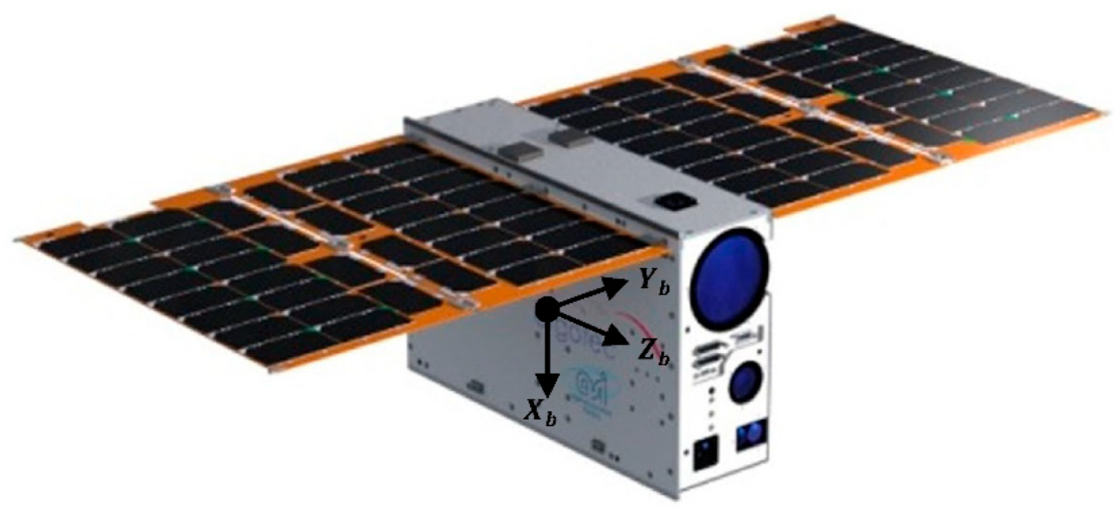
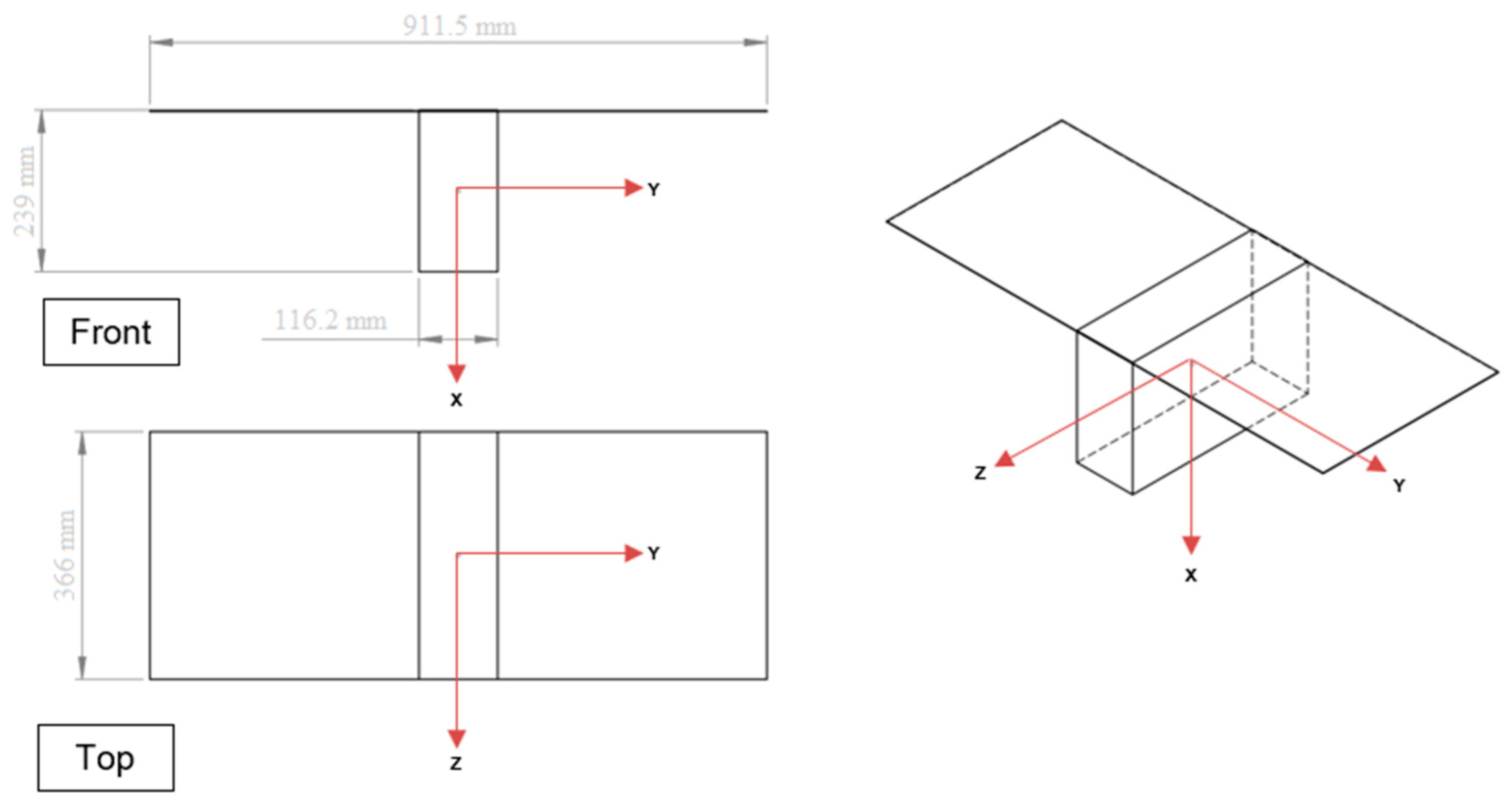
2.2. The Spacecraft
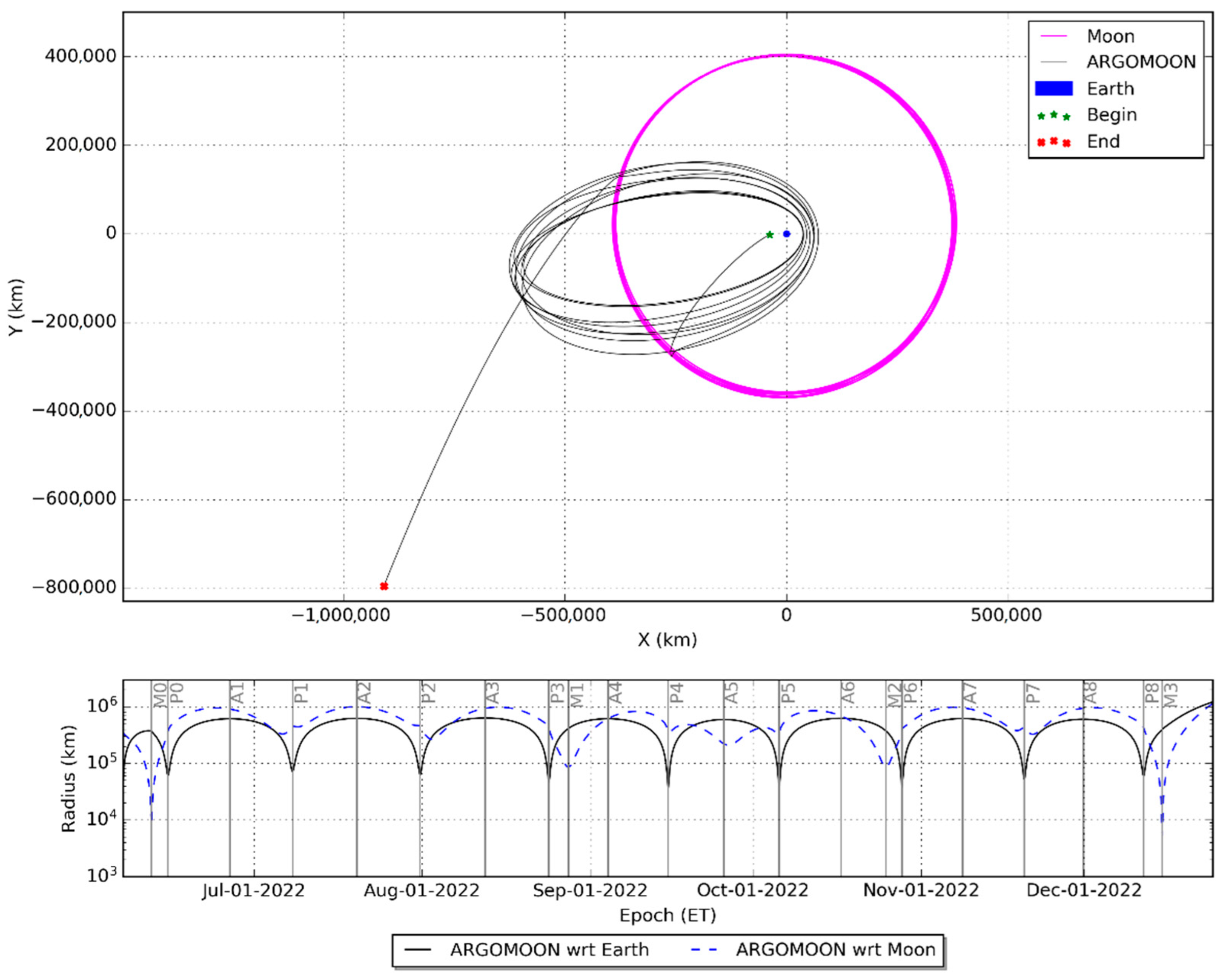
2.3. Trajectory
2.4. Navigation Requirements
- Impact avoidance: the S/C shall not fly below the threshold altitudes of 1000 km with respect to the Earth and 100 km with respect to the Moon. The requirement applies to the whole mission and can become significant at the perigees and fly-bys of the Moon.
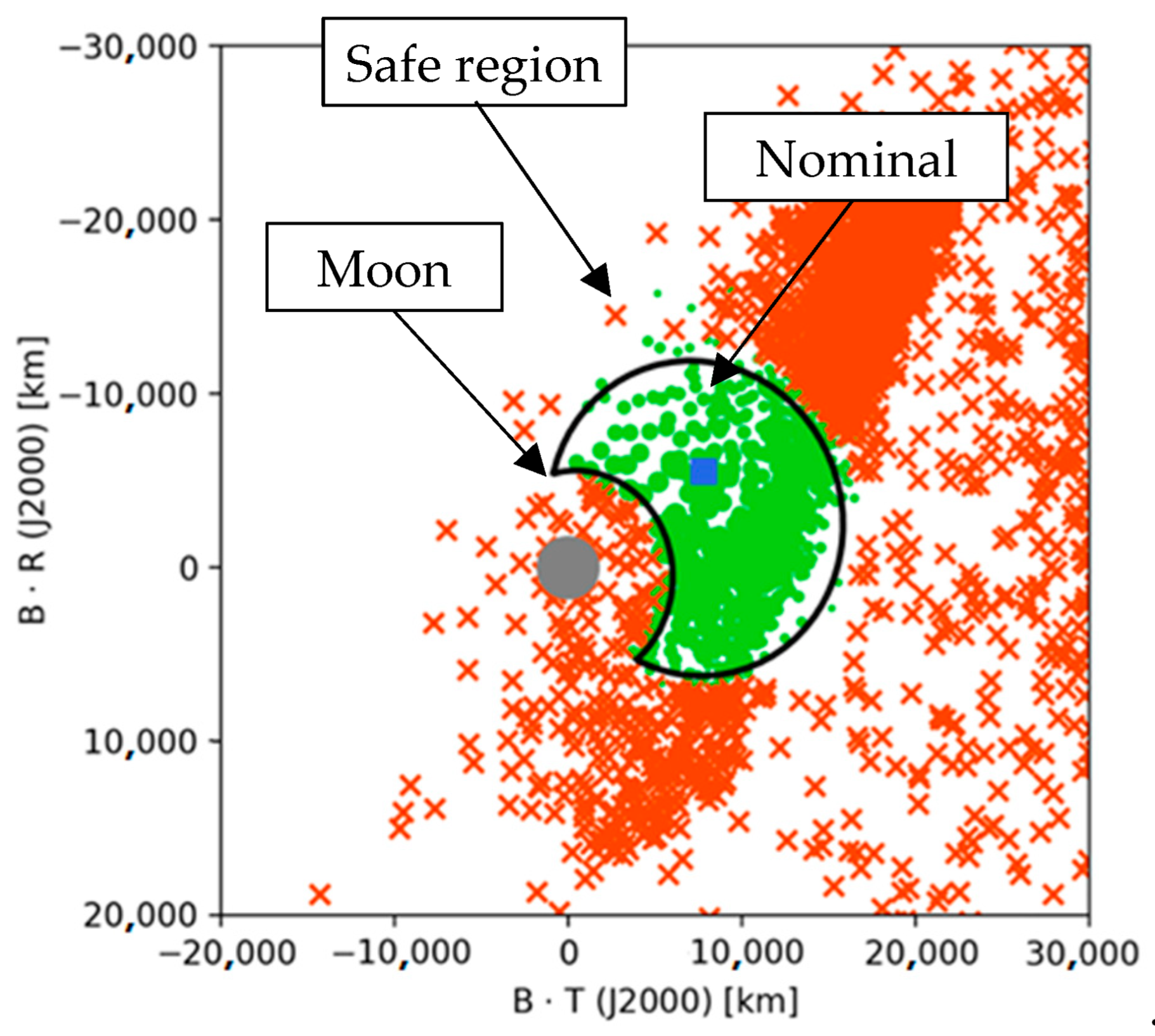
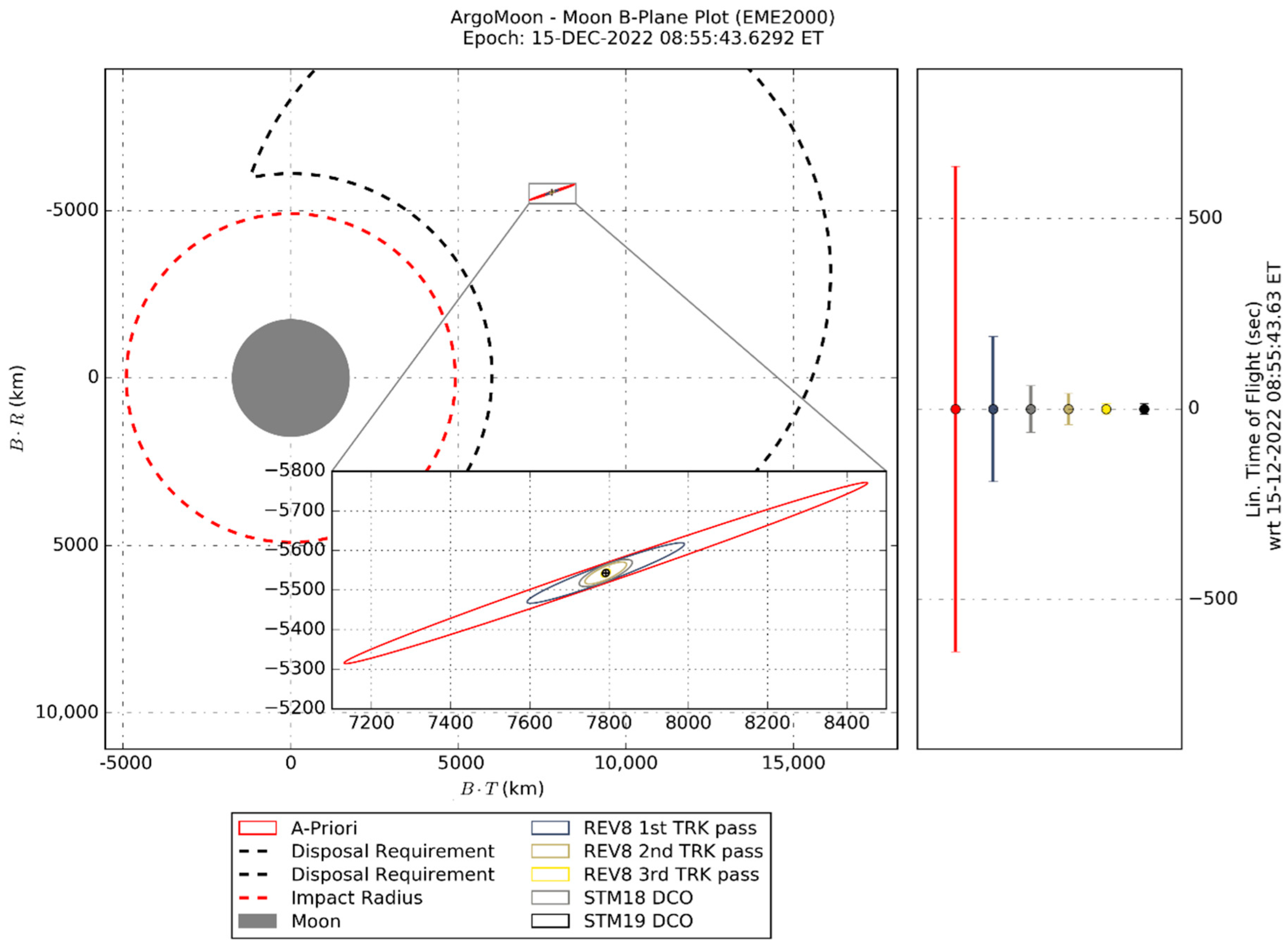
- Heliocentric disposal: the S/C shall reach the heliocentric disposal orbit after the last fly-by of the Moon. The ranges of tolerance for the disposal conditions have been determined through a Monte Carlo analysis with the requirement of having a low probability of crossing the Earth’s sphere of influence in successive years. The disposal requirement is displayed in Figure 3, where the green dots are the samples with a correct disposal and the red crosses are the ones that do not satisfy the requirement.
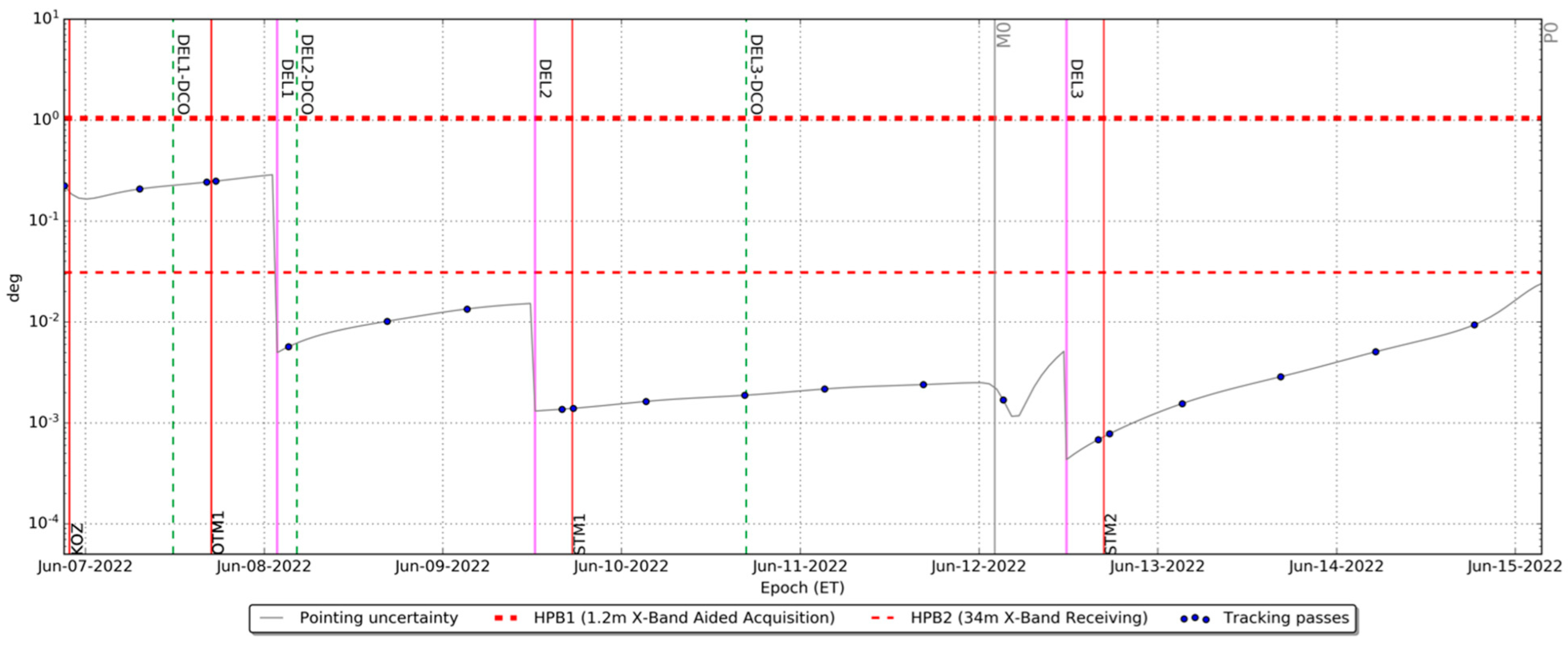
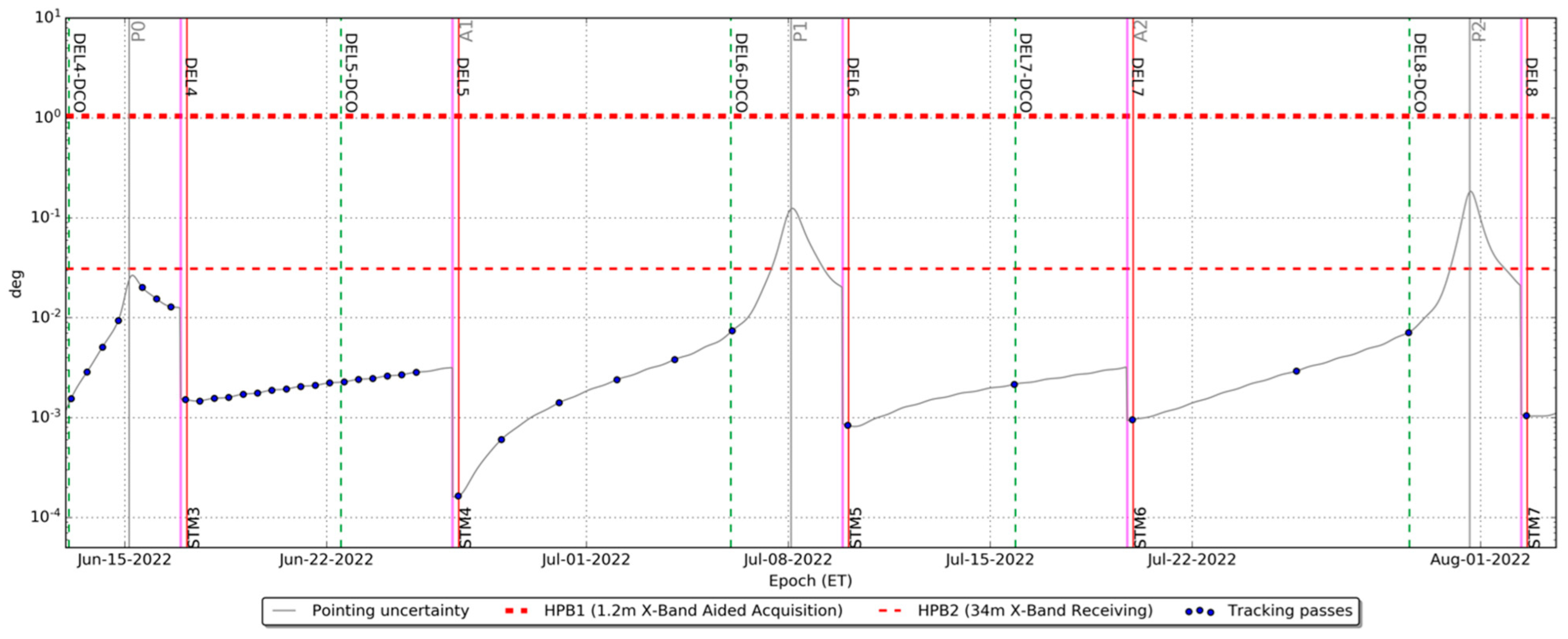
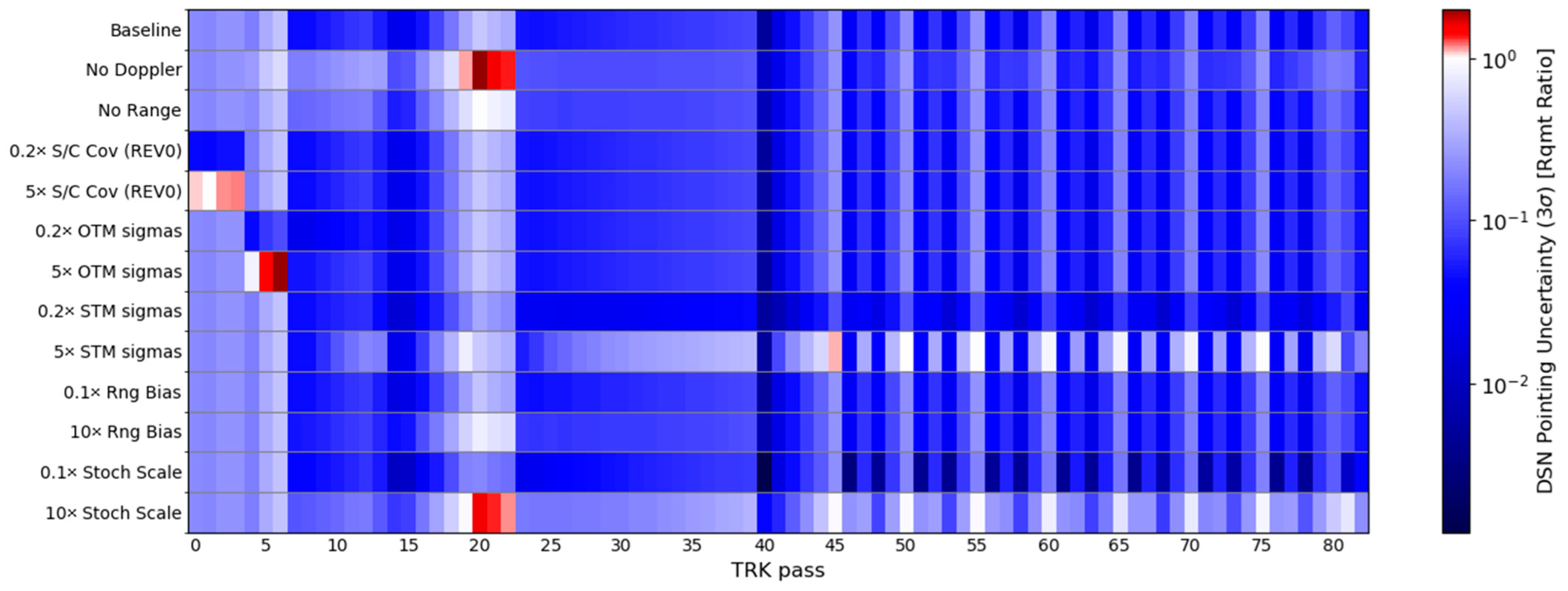
- DSN pointing uncertainty: to ensure the link with the DSN 34 m antennas, the pointing uncertainty due to S/C orbit determination shall be lower than 0.031 deg, which corresponds to the Half Power Beamwidth (HPB) of the antenna at X-band [15]. However, during the first day of the mission, the threshold value of the pointing uncertainty is relaxed to 1.05 deg, which corresponds to half of the HPB of the 34 m dishes equipped with the 1.2 m aided acquisition antenna above the sub-reflector [15].
2.5. Navigation Concept
3. Flight Path Control Analysis
3.1. Uncontrolled Trajectory
3.2. Optimal Control Strategy
4. Orbit Determination Analysis
4.1. Processing Assumptions
4.2. Dynamical Model
4.3. Tracking Schedule
4.4. Filter Configuration
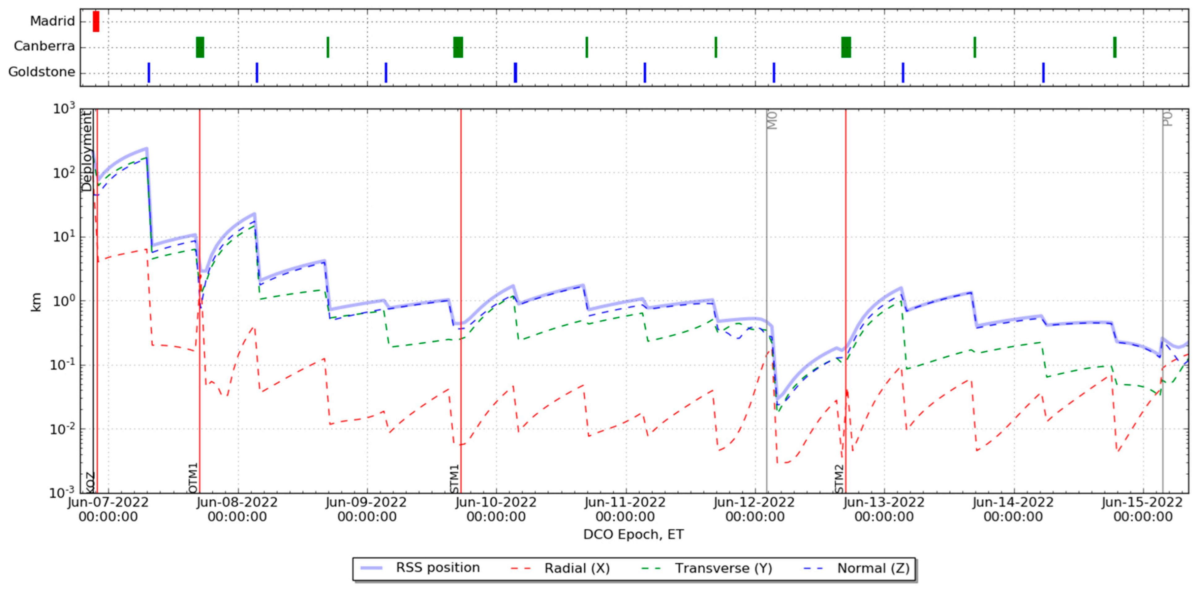
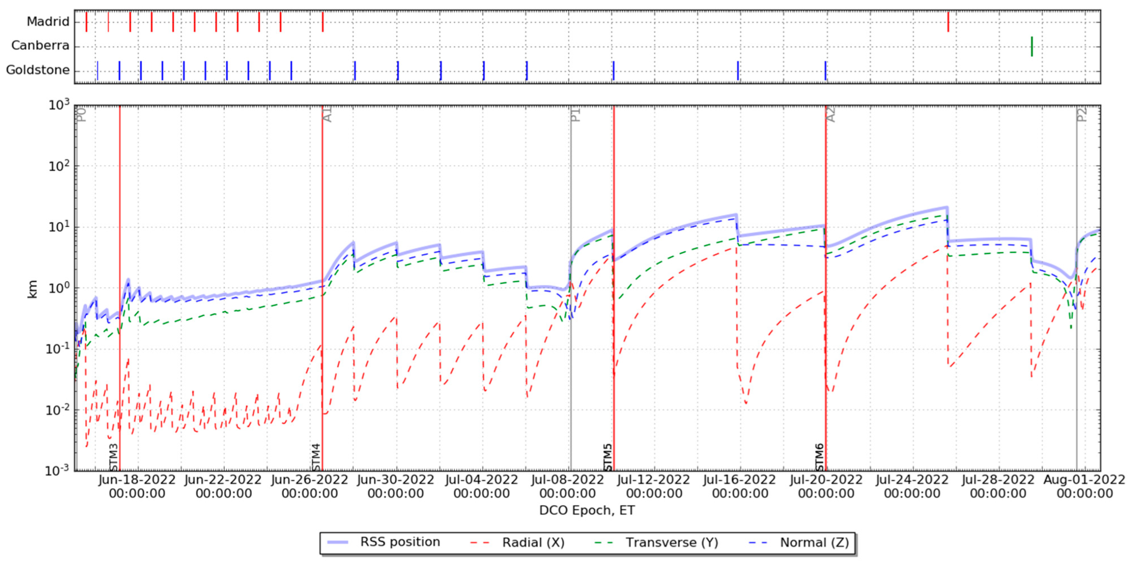
4.5. Baseline Results
5. Sensitivity Analysis
6. Conclusions
Author Contributions
Funding
Data Availability Statement
Acknowledgments
Conflicts of Interest
References
- Puig-Suari, J.; Turner, C.; Ahlgren, W. Development of the standard CubeSat deployer and a CubeSat class PicoSatellite. In IEEE Aerospace Conference Proceedings; Cat. No.01TH8542; IEEE: Piscataway, NJ, USA, 2001; Volume 1, pp. 1/347–1/353. [Google Scholar] [CrossRef]
- Karatekin, Ö.; Le Bras, E.; van Wal, S.; Herique, A.; Tortora, P.; Ritter, B.; Scoubeau, M.; Manuel Moreno, V. Juventas Cubesat for the hera mission. In Proceedings of the 15th Europlanet Science Congress 2021, Online, 13–24 September 2021. [Google Scholar] [CrossRef]
- Dotto, E.; Della Corte, V.; Amoroso, M.; Bertini, I.; Brucato, J.R.; Capannolo, A.; Cotugno, B.; Cremonese, G.; Di Tana, V.; Gai, I.; et al. LICIACube—The Light Italian Cubesat for Imaging of Asteroids in support of the NASA DART mission towards asteroid (65803) Didymos. Planet. Space Sci. 2021, 199, 105185. [Google Scholar] [CrossRef]
- Di Tana, V.; Cotugno, B.; Simonetti, S.; Mascetti, G.; Scorzafava, E.; Pirrotta, S. ArgoMoon: There is a Nano-Eyewitness on the SLS. IEEE Aerosp. Electron. Syst. Mag. 2019, 34, 30–36. [Google Scholar] [CrossRef]
- Schoolcraft, J.; Klesh, A.; Werne, T. MarCO: Interplanetary mission development on a CubeSat scale. In Space Operations: Contributions from the Global Community; Springer: Berlin, Germany, 2017; pp. 221–231. [Google Scholar] [CrossRef]
- Capannolo, A.; Zanotti, G.; Lavagna, M.; Epifani, E.M.; Dotto, E.; Della Corte, V.; Gai, I.; Zannoni, M.; Amoroso, M.; Pirrotta, S. Challenges in Licia Cubesat trajectory design to support dart mission science. Acta Astronaut. 2021, 182, 208–218. [Google Scholar] [CrossRef]
- Gardner, T.; Cheetham, B.; Forsman, A.; Meek, C.; Kayser, E.; Parker, J.; Thompson, M.; Latchu, T.; Rogers, R.; Bryant, B.; et al. CAPSTONE: A CubeSat Pathfinder for the Lunar Gateway Ecosystem. In Proceedings of the Small Satellite Conference, Online, 7–12 August 2021. [Google Scholar]
- Cervone, A.; Topputo, F.; Speretta, S.; Menicucci, A.; Turan, E.; Di Lizia, P.; Massari, M.; Franzese, V.; Giordano, C.; Merisio, G.; et al. LUMIO: A CubeSat for observing and characterizing micro-meteoroid impacts on the Lunar far side. Acta Astronaut. 2022, 195, 309–317. [Google Scholar] [CrossRef]
- De Grossi, F.; Marzioli, P.; Cho, M.; Santoni, F.; Circi, C. Trajectory optimization for the Horyu-VI international lunar mission. Astrodynamics 2021, 5, 263–278. [Google Scholar] [CrossRef]
- Smith, R.M.; Merancy, N.; Krezel, J. Exploration Missions 1, 2, and Beyond: First Steps Toward a Sustainable Human Presence at the Moon. In Proceedings of the IEEE Aerospace Conference, Big Sky, MT, USA, 2–9 March 2019; pp. 1–12. [Google Scholar] [CrossRef]
- McIntosh, D.; Baker, J.; Matus, J. The NASA Cubesat Missions Flying on Artemis-1. In Proceedings of the 34th Annual Small Satellite Conference, Logan, UT, USA, 1–6 August 2020; p. SSC20-WKVII-02. [Google Scholar]
- Dahir, A.; Gillard, C.; Wallace, B.; Sobtzak, J.; Palo, S.; Kubitschek, D. Forgoing Time and State—The Challenge for CubeSats on Artemis-1. JoSS J. Small Satell. 2021, 10, 1049–1060. [Google Scholar]
- Thornton, C.L.; Border, J.S. Radiometric Tracking Techniques for Deep-Space Navigation; John Wiley & Sons: Hoboken, NJ, USA, 2003. [Google Scholar] [CrossRef]
- Kobayashi, M.; Holmes, S.; Yarlagadda, A.; Aguirre, F.; Chas, M.; Angkasa, K.; Burgett, B.; McNally, L.; Dobreva, T.; Satorius, E. The Iris Deep-Space Transponder for the SLS EM-1 Secondary Payloads. IEEE Aerosp. Electron. Syst. Mag. 2019, 34, 34–44. [Google Scholar] [CrossRef]
- Slobin, S.; Pham, T. 34-m BWG Stations Telecommunications Interfaces. In DSN Telecommunications Link Design Handbook (810-005); NASA: Washington, DC, USA, 2010. [Google Scholar]
- Farnocchia, D.; Eggl, S.; Chodas, P.; Giorgini, J.; Chesley, S. Planetary encounter analysis on the B-plane: A comprehensive formulation. Celest. Mech. Dyn. Astron. 2019, 131, 36. [Google Scholar] [CrossRef]
- Bierman, G. Factorization Methods for Discrete Sequential Estimation; Dover Publications Inc.: Mineola, NY, USA, 1977; p. 11501. [Google Scholar] [CrossRef]
- Moyer, T. Formulation for Observed and Computed Values of Deep Space Network Data Types for Navigation; JPL Publication 00-7; Monograph 2 of Deep-Space Communications and Navigation Series; John Wiley & Sons: Hoboken, NJ, USA, 2005. [Google Scholar]
- Iess, L.; Di Benedetto, M.; James, N.; Mercolino, M.; Simone, L.; Tortora, P. Astra: Interdisciplinary study on enhancement of the end-to-end accuracy for spacecraft tracking techniques. Acta Astronaut. 2014, 94, 699–707. [Google Scholar] [CrossRef]
- Bar-Sever, Y.; Jacobs, C.; Keihm, S.; Lanyi, G.; Naudet, C.; Rosenberger, H.; Runge, T.; Tanner, A.; Vigue-Rodi, Y. Atmospheric media calibration for the deep space network. Proc. IEEE 2007, 95, 2180–2192. [Google Scholar] [CrossRef]
- Evans, S.; Taber, W.; Drain, T.; Smith, J.; Wu, H.; Guevara, M.; Sunseri, R.; Evans, J. MONTE: The next generation of mission design & navigation software. CEAS Space J. 2018, 10, 79–86. [Google Scholar] [CrossRef]
- Gomez Casajus, L.; Zannoni, M.; Modenini, D.; Tortora, P.; Nimmo, F.; van Hoolst, T.; Buccino, D.; Oudrhiri, K. Updated Europa gravity field and interior structure from a reanalysis of Galileo tracking data. Icarus 2021, 358, 114187. [Google Scholar] [CrossRef]
- Tortora, P.; Zannoni, M.; Hemingway, D.; Nimmo, F.; Jacobson, R.; Iess, L.; Parisi, M. Rhea gravity field and interior modeling from Cassini data analysis. Icarus 2016, 264, 264–273. [Google Scholar] [CrossRef]
- Zannoni, M.; Hemingway, D.; Gomez Casajus, L.; Tortora, P. The gravity field and interior structure of Dione. Icarus 2020, 345, 113713. [Google Scholar] [CrossRef]
- Gomez Casajus, L.; Ermakov, A.; Zannoni, M.; Keane, J.; Stevenson, D.; Buccino, D.; Durante, D.; Parisi, M.; Park, R.; Tortora, P.; et al. Gravity Field of Ganymede after the Juno Extended Mission. Geophys. Res. Lett. 2022; accepted. [Google Scholar]
- Vaquero, M.; Hahn, Y.; Roth, D.; Wong, M. A Linear Analysis for the Flight Path Control of the Cassini Grand Finale Orbits. In Proceedings of the International Symposium on Space Flight Dynamics, Matsuyama, Japan, 3–9 June 2017. [Google Scholar]
- Wagner, S.; Goodson, T. Execution-error modeling and analysis of the Cassini-Huygens spacecraft through 2007. In Spaceflight Mechanics 2008, Proceedings of the AAS/AIAA Space Flight Mechanics, Galveston, TX, USA, 27–31 January 2008; American Astronautical Society: San Diego, CA, USA, 2008. [Google Scholar]
- Folkner, W.; Williams, J.; Boggs, D.; Park, R.; Kuchynka, P. The Planetary and Lunar Ephemerides DE430 and DE431. Interplanet. Netw. Prog. Rep. 2014, 196, 42–196. [Google Scholar]
- Cagle, C.; Scott, C.; Berner, J.; Beyer, P.; Guerrero, A.; Hames, P.; Medeiros, T.; Bhanji, A. DSN Mission Service Interfaces, Policies, and Practices (MSIPP); 875-0001, Rev. G, JPL D-26688; NASA: Washington, DC, USA, 2015.


| Event | Event Epoch | Details |
|---|---|---|
| Bus Stop 1 (BS1) | Launch + 3 h 54 min | First CubeSats dispensing phase |
| Bus Stop 2 (BS2) | Launch + 6 h 59 min | Last ArgoMoon observed deployment phase |
| Deployment (TD) | BS1 + 6 min | Release of ArgoMoon from the ICPS (close to BS1) |
| Transponder ON | TD + 30 min | ArgoMoon starts to communicate with DSN |
| KOZ | TD + 75 min | Keep Out Zone maneuver to drift away from the ICPS |
| OTM1 | ~TD + 20 h | Maneuver to trim the first fly-by of the Moon (M0) |
| M0 | ~TD + 5.23 days | First fly-by of the Moon: C/A at 7773 km |
| M1 | ~TD + 82.08 days | Mid-course fly-by of the Moon: C/A at 86,051 km |
| M2 | ~TD + 104.61 days | Mid-course fly-by of the Moon: C/A at 84,594 km |
| M3 | ~TD + 191.51 days | Last fly-by of the Moon: C/A at 5261 km |
| EOM | End of the mission | |
| Pi (i = 0,1…8) | Perigees | Total number of perigees: 9 |
| Ai (i = 0,1…8) | Apogees | Total number of apogees: 9 |
| REV0 | to P0 | First revolution that encompasses the fly-by M0 |
| REVi (i = 1,8) | Pi to Pi + 1 | Revolutions around the Earth (i.e., REV3: from P2 to P3) |
| REV9 | P8 to EOM | Last revolution that encompasses the fly-by M3 |
| Injection covariance | ICPS state (Earth-RTN) uncertainty (3-sigma) at BS1 epoch: | |||||
| X (km) | Y (km) | Z (km) | VX (km/s) | VY (km/s) | VZ (km/s) | |
| 30.0 | 60.0 | 15.0 | 0.0021 | 0.0027 | 0.0042 | |
| Maneuvers execution error | Gates Model applied to both OTMs and STMs. | |||||
| Mis-modeling and OD error | OD covariance mapped from the maneuver’s DCO to the aimpoint. | |||||
| Maneuvers execution error | Error Component (Per Axis) | ArgoMoon PS | |
| Magnitude | Fixed (m/s) Proportional (%) | 0.011 3.5 | |
| Pointing | Fixed (m/s) Proportional (deg) | 0.011 1.1 |
| Maneuver | Epoch | Aimpoint | Coordinates (EME2000) | ΔV Mean (m/s) | ΔV 99% (m/s) |
|---|---|---|---|---|---|
| OTM1 | N/A: deterministic open-loop burn | 11.031 | 11.921 | ||
| STM1 | OTM1 + 48 h | M0 | B.R, B.T, TCA | 5.706 | 17.306 |
| STM2 | P0−48 h | A1 | X, Y, Z | 4.527 | 18.315 |
| STM3 | P0 + 48 h | A1 | X, Y, Z | 0.405 | 2.195 |
| STM4 | A1 | P1 | VX, VY, VZ | 0.398 | 1.174 |
| STM5 | P1 + 48 h | A2 | X, Y, Z | 0.088 | 0.381 |
| STM6 | A2 | P2 | VX, VY, VZ | 0.106 | 0.312 |
| STM7 | P2 + 48 h | A3 | X, Y, Z | 0.067 | 0.191 |
| STM8 | A3 | P3 | VX, VY, VZ | 0.096 | 0.269 |
| STM9 | P3 + 48 h | A4 | X, Y, Z | 0.061 | 0.153 |
| STM10 | A4 | P4 | VX, VY, VZ | 0.088 | 0.238 |
| STM11 | P4 + 48 h | A5 | X, Y, Z | 0.053 | 0.141 |
| STM12 | A5 | P5 | VX, VY, VZ | 0.086 | 0.245 |
| STM13 | P5 + 48 h | A6 | X, Y, Z | 0.047 | 0.122 |
| STM14 | A6 | P6 | VX, VY, VZ | 0.082 | 0.231 |
| STM15 | P6 + 48 h | A7 | X, Y, Z | 0.073 | 0.216 |
| STM16 | A7 | P7 | VX, VY, VZ | 0.093 | 0.251 |
| STM17 | P7 + 48 h | A8 | X, Y, Z | 0.057 | 0.152 |
| STM18 | A8 | M3 | B.R, B.T, TCA | 0.074 | 0.206 |
| STM19 | P8 + 12 h | M3 | B.R, B.T, TCA | 0.146 | 0.425 |
| Total cumulated statistical ΔV: | 23.287 | 49.443 | |||
| Arc data | Tracking data of a single REV (between two perigees): | |
| Tracking data X/X band | Doppler | 2-way, 60 s of integration time |
| Range | 2-way, 1 observable every 300 s | |
| Data noise and weights | Doppler | 0.1 mm/s at 60 s of integration time (2.81 mHz at X-band) |
| Range | 2 m | |
| Stochastic accelerations | per axis, uncorrelated white noise, 8 h of batch time | |
| Orbital Maneuvers | DCO | 96 h before the maneuver’s epoch (nominal) 24 h before the maneuver’s epoch (minimum) |
| Tracking | No tracking data during the maneuver execution | |
| REV0 epoch state covariance | ICPS state (Earth-RTN) uncertainty (3-sigma) at BS1 epoch (Table 2) | |
| REV1 to REV9 epoch state covariance | Previous arc’s mapped state covariance scaled by a safety factor of 4 | |
| Component | Specular Reflectivity (ρ) | Diffusive Reflectivity (δ) |
|---|---|---|
| Bus faces | 0.0 | 0.25 |
| Solar arrays | 0.115 | 0.25 |
| Parameter | Unit | A priori Uncertainty | Estimated/Considered | |
|---|---|---|---|---|
| S/C epoch state (REV0) | - | ICPS state covariance at BS1 (Table 5:) | Estimated | |
| S/C epoch state (REV1-REV9) | - | Estimated covariance mapped from previous arc, multiplied by 4 | Estimated | |
| Solar Radiation Pressure Scale Factor | - | 50% | Estimated | |
| Deterministic impulse burns (OTM) | ΔV | m/s | 10% of nominal | Estimated |
| Ra | deg | 1.1 | Estimated | |
| Dec | deg | 1.1 | Estimated | |
| Time | s | 3.0 | Estimated | |
| Statistical impulse burns (STM) | ΔV(X) | m/s | 0.011 | Estimated |
| ΔV(Y) | m/s | 0.011 | Estimated | |
| ΔV(Z) | m/s | 0.011 | Estimated | |
| Time | s | 3.0 | Estimated | |
| Stochastic accelerations | X/Y/Z | km/s2 | 10−11, 8-h batches | Estimated |
| Range Bias (per pass) | m | 2 | Estimated | |
| Earth GM | km3/s2 | 5.0 × 10⁻⁴ | Considered | |
| Moon GM | km3/s2 | 1.4 × 10⁻⁴ | Considered | |
| DSN station locations (per axis) | cm | 3 | Considered | |
| Troposphere path delay (wet/dry) | cm | 1/1 | Considered | |
| Ionosphere path delay (day/night) | cm | 5/1 | Considered | |
| Earth Polar Motion X/Y | deg | 8.6 × 10⁻⁷ | Considered | |
| UT1 bias | s | 2.5 × 10⁻⁴ | Considered | |
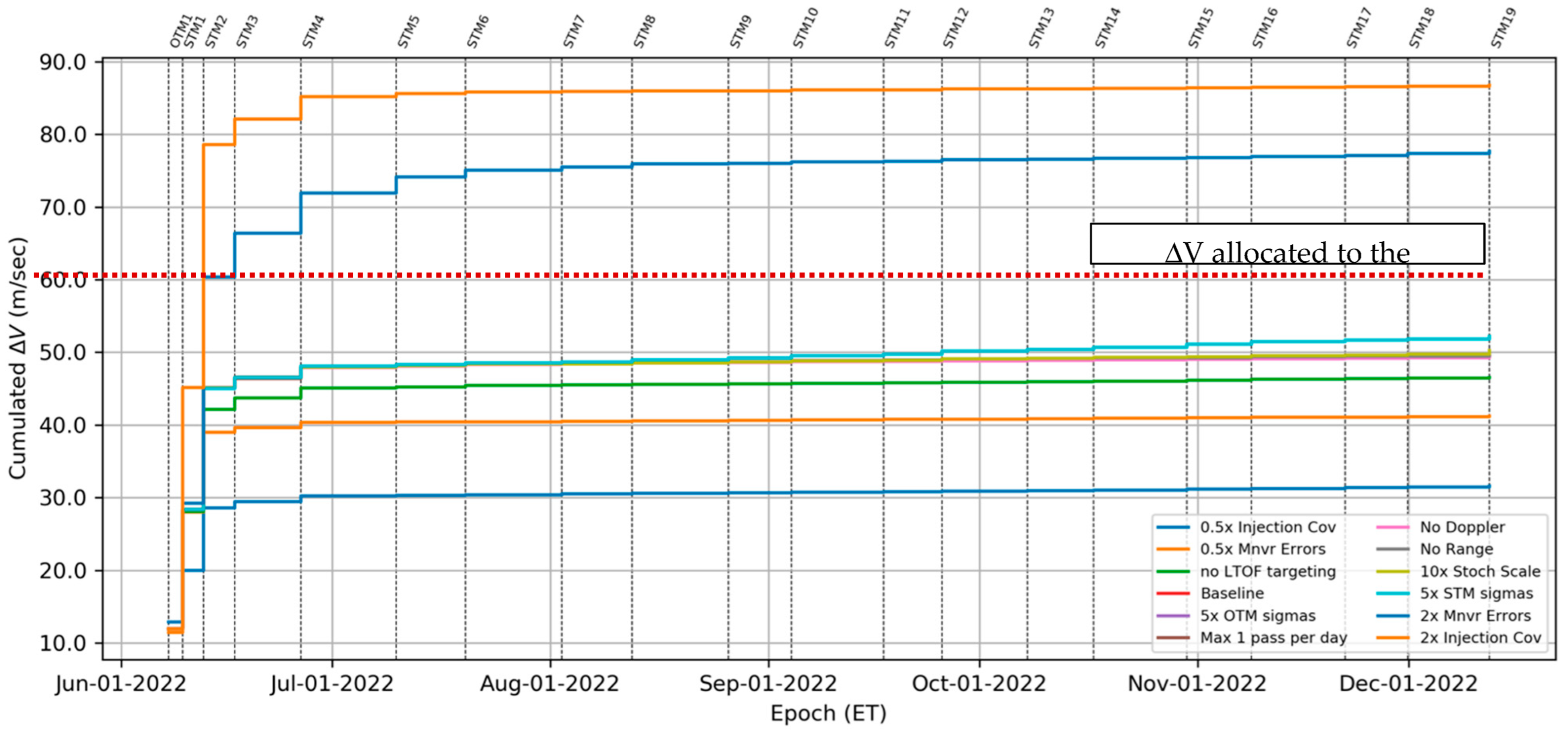
| Case | Mean (m/s) | Sigma (m/s) | ΔV 99% (m/s) |
|---|---|---|---|
| Baseline | 23.3 | 7.6 | 49.5 |
| 0.5 × Injection Covariance | 18.2 | 3.9 | 31.6 |
| 0.5 × Maneuvers Execution Error | 21.4 | 6.2 | 41.3 |
| No LTOF targeting | 22.1 | 7.2 | 46.6 |
| 5 × OTM1 sigmas | 23.3 | 7.7 | 49.5 |
| Maximum 1 pass per day | 23.4 | 7.6 | 49.6 |
| No Doppler data | 23.6 | 7.6 | 49.6 |
| No Range data | 23.5 | 7.6 | 49.8 |
| 10 × Stochastic sigmas | 24.4 | 7.6 | 50.3 |
| 5 × STM sigmas | 26.6 | 7.6 | 52.3 |
| 2 × Maneuvers Execution Error | 30.1 | 12.9 | 77.7 |
| 2 × Injection Covariance | 34.0 | 15.2 | 86.8 |
Publisher’s Note: MDPI stays neutral with regard to jurisdictional claims in published maps and institutional affiliations. |
© 2022 by the authors. Licensee MDPI, Basel, Switzerland. This article is an open access article distributed under the terms and conditions of the Creative Commons Attribution (CC BY) license (https://creativecommons.org/licenses/by/4.0/).
Share and Cite
Lombardo, M.; Zannoni, M.; Gai, I.; Gomez Casajus, L.; Gramigna, E.; Manghi, R.L.; Tortora, P.; Di Tana, V.; Cotugno, B.; Simonetti, S.; et al. Design and Analysis of the Cis-Lunar Navigation for the ArgoMoon CubeSat Mission. Aerospace 2022, 9, 659. https://doi.org/10.3390/aerospace9110659
Lombardo M, Zannoni M, Gai I, Gomez Casajus L, Gramigna E, Manghi RL, Tortora P, Di Tana V, Cotugno B, Simonetti S, et al. Design and Analysis of the Cis-Lunar Navigation for the ArgoMoon CubeSat Mission. Aerospace. 2022; 9(11):659. https://doi.org/10.3390/aerospace9110659
Chicago/Turabian StyleLombardo, Marco, Marco Zannoni, Igor Gai, Luis Gomez Casajus, Edoardo Gramigna, Riccardo Lasagni Manghi, Paolo Tortora, Valerio Di Tana, Biagio Cotugno, Simone Simonetti, and et al. 2022. "Design and Analysis of the Cis-Lunar Navigation for the ArgoMoon CubeSat Mission" Aerospace 9, no. 11: 659. https://doi.org/10.3390/aerospace9110659
APA StyleLombardo, M., Zannoni, M., Gai, I., Gomez Casajus, L., Gramigna, E., Manghi, R. L., Tortora, P., Di Tana, V., Cotugno, B., Simonetti, S., Patruno, S., & Pirrotta, S. (2022). Design and Analysis of the Cis-Lunar Navigation for the ArgoMoon CubeSat Mission. Aerospace, 9(11), 659. https://doi.org/10.3390/aerospace9110659