Article

Generalized Quantitative Stability Analysis of Time-Dependent Comprehensive Rotorcraft Systems

1
Department of Mechanical Engineering, Imperial College London, London SW7 2AZ, UK
2
Department of Aerospace Science and Technology, Politecnico di Milano, 20156 Milan, Italy
*
Author to whom correspondence should be addressed.
Aerospace 2022, 9(1), 10; https://doi.org/10.3390/aerospace9010010
Submission received: 23 October 2021 / Revised: 21 December 2021 / Accepted: 22 December 2021 / Published: 24 December 2021
(This article belongs to the Special Issue Rotorcraft)

Abstract

:
Rotorcraft stability is an inherently multidisciplinary area, including aerodynamics of rotor and fuselage, structural dynamics of flexible structures, actuator dynamics, control, and stability augmentation systems. The related engineering models can be formulated with increasing complexity due to the asymmetric nature of rotorcraft and the airflow on the rotors in forward flight conditions. As a result, linear time-invariant (LTI) models are drastic simplifications of the real problem, which can significantly affect the evaluation of the stability. This usually reveals itself in form of periodic governing equations and is solved using Floquet’s method. However, in more general cases, the resulting models could be non-periodic, as well, which requires a more versatile approach. Lyapunov Characteristic Exponents (LCEs), as a quantitative method, can represent a solution to this problem. LCEs generalize the stability solutions of the linear models, i.e., eigenvalues of LTI systems and Floquet multipliers of linear time-periodic (LTP) systems, to the case of non-linear, time-dependent systems. Motivated by the need for a generic tool for rotorcraft stability analysis, this work investigates the use of LCEs and their sensitivity in the stability analysis of time-dependent, comprehensive rotorcraft models. The stability of a rotorcraft modeled using mid-fidelity tools is considered to illustrate the equivalence of LCEs and Floquet’s characteristic coefficients for linear time-periodic problems.

1. Introduction

Rotorcraft use rotating blades to generate the loads required for flight, i.e., lift, propulsion, and control, as needed to take-off and land vertically, as well as hover [1]. They can fulfill many roles that fixed-wing aircraft cannot perform as effectively, such as search and rescue, if they can at all. To provide a sufficient level of thrust at hover and low airspeeds, a relative motion must be maintained between the rotating wings and the air. Rotors should have a long enough span to enable the efficient lifting, propulsion, and control of the vehicle [2]. These three fundamental functions significantly affect each other, and lead to cross-couplings, which result in more complex flight physics compared to fixed-wing aircraft [3].
Stability assessment is an important task in helicopter design, especially considering that from an aeromechanical viewpoint they are inherently unstable [4]. A specific form of complexity arises from the rotation of the blades in forward flight, which induces periodic aerodynamic loading on the rotor blades. Additionally, blades in the advancing azimuthal range add their rotational velocity with a component of the forward flight speed of the vehicle, and exhibit substantial compressibility effects at high forward speeds, with the blade tip approaching Mach 1. Conversely, blades in the other half of the azimuth move in a direction opposite to that of the vehicle, resulting in low relative speed, the need for high angles of attack to compensate for the reduction of lift, proximity to stalled flow, and even reverse flow conditions near the blade root. As a consequence of extended stall and reverse flow regions, high levels of drag result, with a significant drop in the lift. In addition to the time-dependence of aerodynamic origin, similar effects also occur if an unbalance is present in the rotating elements. The latter can usually happen as a result of deviations from nominal mass distribution, or aerodynamic shape distortion [5]. Another source could be a malfunction of one of the repetitive mechanical elements, such as lead-lag dampers [6]. Whatever the reason, the loss of symmetry in the rotation field results in
  • alternating loads that excite the fuselage, and
  • alternating system properties leading to a time-dependent system.
While the former represents a forced vibration problem, the latter results in a time-variant problem, whose stability analysis is more difficult.
In dynamical systems, the study of nearby solutions of an equilibrium point is referred to as stability [7]. In other words, the system response after a perturbation of the system’s state is introduced about an equilibrium condition [8]. There are several methods to assess the stability of a system. A conventional one is perturbing the system through typical input or disturbance sources and observing the free-decay characteristic. This could be performed by conducting experiments on a manufactured product or through computer simulations. Alternatively, spectral methods exist, which quantify the decaying behaviour of independent components of the solution, which is referred to as the system’s exponential multipliers or characteristic exponents. Once the stability spectrum that quantifies stability is obtained, it is straightforward to interpret the results and track the changes in stability characteristics with the evolution of the design. Besides, the spectral methods are also suitable for the analytical estimation of the sensitivity of stability estimates. This work focuses on spectral methods of estimating stability.
The validity of rotorcraft stability estimation is defined by the capability of mathematical and numerical tools used in evaluating the stability and the simplifications made during the process. For the linear, time-invariant (LTI) case, stability can be assessed using eigenanalysis of the system’s matrix. A more difficult case is that of linear, time-periodic (LTP) systems, a special class of linear, time-variant (LTV) problems, which can be considered to address the intrinsic periodicity of idealized rotorcraft, especially originating from the main rotor’s aerodynamics in non-axial flow conditions, or dissimilarities in the rotor components, as in ground resonance with degraded dampers. A widespread tool, in this case, is Floquet’s theory, which represents a natural extension of eigenvalue analysis for LTP systems [9]. The eigenvalue decomposition for LTI systems and Floquet analysis of LTP problems may successfully evaluate stability in several flight conditions; however, rotorcraft dynamics is generally described by non-linear, generically time-dependent equations [10]. Therefore, these methods imply simplifications when the system is neither time-invariant nor periodic. For these reasons, capturing the effects of time-dependence in rotorcraft stability could provide more insight into increasingly complex rotorcraft stability problems.
To achieve a generalized framework for the stability analysis of rotorcraft, a technique that can estimate the stability of time-dependent systems is required. This method is further needed to require no simplifications regarding time-dependence nor any assumption of periodicity. Additionally, the technique should give the same results and interpretation when applied to relatively simple models of time-invariant and periodic systems. Lyapunov Characteristic Exponents (LCE) satisfy all these requirements and can represent a universal framework for rotorcraft aeroelastic stability. LCEs are the indicators of the stability properties of non-linear, time-dependent differential equations [11]. Therefore, no simplifications are required concerning the time-dependence of the system, paving the way for a more versatile and accurate assessment of rotorcraft stability.
Concerning their application to rotorcraft aeromechanics, LCEs and their sensitivity were studied for the first time for specific non-linear engineering systems and subcomponents in Refs. [12,13]. This work extends their use to time-dependent high fidelity rotorcraft problems as a quantitative stability assessment method. The rest of the paper is organized as follows. Section 2 briefly introduces Lyapunov Characteristic Exponents and their practical computation. Two time-dependent example problems are utilized in Section 3 to illustrate the approach, where the LCE stability indicators are compared with the conventional Floquet multiplier. Conclusions are finally drawn in Section 4.

2. Method

This section illustrates the theory and estimation of Lyapunov Characteristic Exponents (or Lyapunov Exponents, in short) and their sensitivity.

2.1. Lyapunov Characteristic Exponents

An LTI dynamical system can be represented in state-space form as:
x ˙ = A x , x ( t 0 ) = x 0 ,
where vector x R n contains the n states of the system, and matrix A R n × n is referred to as the state-space matrix. When matrix A is not singular, x = 0 (the trivial solution) is the unique equilibrium condition. In this case, the stability of the LTI system in Equation (1) is estimated by the eigenvalues of the state-space matrix A [14]. Three fundamental outcomes may originate from this consideration.
  • First, the time response of the system converges to zero, which happens when all eigenvalues have a negative real part.
  • Second, the system responds in a divergent manner when some eigenvalues have a positive real part.
  • Third, a periodic orbit can be the resulting motion in the presence of purely imaginary eigenvalues.
A combination of these fundamental response types can occur, as well [15]. Since only one equilibrium point exists, which is trivial, the stability properties of all possible solutions of x are equivalent to those of the trivial solution. Although the time response amplitude of the system depends on the initial conditions [16], the stability characteristics, i.e., being divergent, convergent, or periodic, do not depend on them.
For LTP systems, the same remarks are valid, as well. The only difference is the need to consider, instead of the state-space matrix A , the monodromy matrix H , which represents the state transition matrix (STM) over one period (often referred to as Floquet transition matrix), i.e., the result of integrating the problem
H ˙ = A ( t ) H
over a period from t = 0 to T, with initial conditions H ( 0 ) = I . For an LTI system, the monodromy matrix over the same period T corresponds to
H = e A T .
While LTI and LTP systems can usually provide sufficiently accurate representations of rotorcraft problems for several applications, the relation between the system states x and its rate of change in time x ˙ cannot be limited to being time-invariant or time-periodic. In other words:
x ˙ = f ( x , t ) , x ( t 0 ) = x 0
is a more generic representation of rotorcraft dynamics, where the non-linear function f ( x , t ) governs the system dynamics and can include relations not necessarily time-invariant nor periodic.
To address the more general time-dependence problem, this work suggests the use of Lyapunov Characteristic Exponents (LCEs). LCEs indicate the stability properties of the solutions of differential equations [11,14]. Mathematically speaking, LCEs define the spectrum of the corresponding initial value, or Cauchy, problem. Moreover, Lyapunov’s theory applies also to non-linear time-dependent systems. The stability of trajectories in the state-space can be estimated while integrating their time response. Therefore, Lyapunov Exponents represent a generalization of the stability properties that are familiar in current engineering practice.
By definition, the trajectory of a system is a solution to a differential equation of the form of Equation (4). Special cases occur if the model is linear, i.e., f ( x , t ) = A ( t ) x ( t ) , or time-periodic, i.e., linear with A ( t + T ) = A ( t ) , for a given period T. Time-invariant problems arise when f ( x ) does not explicitly depend on time t. The simplest form is obtained when the problem is simultaneously linear and time-invariant, i.e., f ( x ) = A x .
Consider the system with x ˙ = f ( x , t ) , where the previously introduced vector x R n contains the states, t R is the time, and f R n + 1 R n is a non-linear time-dependent function. For a solution x ( t ) originating from initial conditions x ( 0 ) = x 0 , the LCEs λ i are defined as:
λ i = lim t 1 t log | | i x ( t ) | | | | i x ( t 0 ) | | ,
where i x ( t ) represents the growth of the ith axis of the ellipsoid that evolves from an initially infinitesimal n-dimension sphere. The evolution happens according to the map f / x , tangent to f along the solution trajectory x ( t ) . In other words, i x ( t ) is the solution of the linear, time-dependent problem
i x ˙ ( t ) = f / x ( x ( t ) , t ) i x ( t ) ,
with initial conditions i x ( t 0 ) = i x 0 .
Equation (5) can be simplified by splitting the log function of Equation (5) as:
λ i = lim t 1 t log | | i x ( t ) | | lim t 1 t log | | i x ( t 0 ) | | .
The second limit involves a constant, | | i x ( t 0 ) | | , divided by time t, which, in the limit, approaches + , obviously tending to zero. The first limit, thus, defines the ith LCE as:
λ i = lim t 1 t log | | i x ( t ) | | .
Due to the presence of a limit for t in the definition, the practical evaluation of LCEs can only be numerically obtained for a sufficiently long time t. For this reason, the term “LCEs” in the following will rather refer to their estimation for a large enough value of t to reach practical convergence.

2.2. Application to LTP Problems

For an LTV problem, the STM is the solution of
Y ˙ = A ( t ) Y ,
integrated from τ to t with initial conditions, Y ( τ ) = I . When replaced in the LCEs definition, it yields
λ i = lim t 1 t log | | Y ( t , 0 ) i x 0 | | .
When the problem is LTP, the time t can be nondimensionalized with respect to the problem’s period T, namely t = T ψ , yielding
λ i = lim ψ 1 T ψ log | | Y ( T ψ , 0 ) i x 0 | | .
Considering now the limit for discrete values of time, for ψ N + to + , one obtains Y ( T ψ , 0 ) = Y ψ ( T , 0 ) , and, recalling the monodromy matrix resulting from the solution of Equation (2), H = Y ( T , 0 ) , one obtains
λ i = lim ψ 1 T ψ log | | H ψ i x 0 | | ,
and, again, expressing the monodromy matrix in spectral form, namely H = X e B T X 1 , and assuming that i x 0 is its ith eigenvector, namely the ith column of matrix X , one obtains
λ i = lim ψ 1 T ψ log | | i x 0 e β i T ψ | | = Re ( β i ) ,
i.e., the LCEs correspond to the real part of the logarithm of the eigenvalues of the monodromy matrix, divided by the period, T.

2.3. Numerical Estimation of LCEs

Starting from the fundamental work of Benettin et al. [11], several methods have been formulated for the estimation of all LCEs, or at least the largest ones. They can be broadly partitioned into two classes: continuous and discrete. Noteworthy continuous methods include those based on the QR and SVD factorizations, whereas, among the discrete ones, that based on QR is worth mentioning, and will be considered in the rest of this work.
LCE evaluation using continuous formulas suffers from the computational difficulty of dealing with matrices whose coefficients either diverge or go to zero rapidly. As a result, practical formulations have been developed. For example, the discrete QR method is a common technique in LCE calculation. In this method, the LCEs estimates are incrementally updated with the diagonal elements of the matrix R , which is extracted using the QR decomposition of the STM evaluated between two successive time steps.
For a given matrix Y ( t , t j 1 ) from time t j 1 to the consecutive time t, define the state transition of the problem Y ˙ = f / x ( x ( t ) , t ) Y with Y ( t j 1 ) = I . Setting Y j = Y ( t j , t j 1 ) and considering the QR decomposition of Y j Q j 1 implies that Q j R j = Y j Q j 1 . When the R Π j matrix is defined as R Π j = Π k = 0 j R j k , it can be shown that:
Y j Q j 1 R Π j 1 = Q j R j R Π j 1 = Q j R Π j .
Using the above relation, Y j Q j 1 R Π j 1   R Π j can be constructed using only incremental QR decompositions over Y j Q j 1 , which allows limited contraction/expansion over one time-step. Now, the LCEs can be estimated from the R Π j matrix as
λ i = lim j 1 t j log r i i ( t j ) ,
where j N and r i i ( t j ) are the diagonal elements of matrix R ( t j ) = R Π j . Since the product of two upper triangular matrices C = A B is also an upper triangular matrix, the diagonal elements are c i i = a i i b i i . Thus, the log ( c i i ) can be computed incrementally, namely log ( a i i b i i ) = log ( a i i ) + log ( b i i ) . This helps prevent overflow/underflow in numerical computations. Furthermore,
r i i ( t j ) = Π k = 0 j r ( j k ) i i ;
thus,
log ( r i i ( t j ) ) = k = 0 j log ( r k i i ) ,
which leads to
λ i = lim j 1 t j k = 0 j log ( r k i i ) .

2.4. Computation of State Transition Matrix

The discrete QR decomposition method needs the calculation of the state transition matrix, which can be obtained by numerical integration. For a sufficiently small time-step, Equation (4) can be linearized:
δ x ˙ = A ( x ( t ) , t ) δ x ,
where A = f / x results from the partial derivative of the non-linear function f with respect to the state-space variables x . On the other hand, f can be an arbitrary non-linear function of x j (trajectory) and t (time). Therefore, to integrate the STM, the knowledge of the fiducial trajectory is required, i.e., the equations of motion need to be integrated first. The numerical integration of differential equations is a relatively straightforward task; as such, it is not discussed here in detail. However, the computation of the state transition matrix is presented, as its determination is essential for the procedure.
An efficient approach for the evaluation of the state transition matrix is Hsu’s method [17], which is also reported in Reference [18] and followed in this work. The method is applied to LTV problems of the form x ˙ = A ( t ) x by considering a piecewise-constant approximation of matrix A ( t ) , namely A ( x , t ) A ( x ^ , t ^ ) = A ^ with t ^ [ t j , t j + 1 ] , where t j t t j + 1 and x ^ = x ( t ^ ) . The selection of t ^ may slightly alter the resulting STM. Finally, the state transition matrix is readily obtained as
Y ( t , t j ) e A ^ ( t t j ) ,
where an approximation of the matrix exponential may be necessary to improve the computational efficiency, such as truncating the matrix power series.

2.5. Analytical Sensitivity of LCEs

In a dynamical system, especially in the design phase, the rate of change of stability estimates with respect to an evolving or uncertain parameter plays a significant role in assessing the stability characteristics. Such sensitivity is useful to gain insight into the dependence of stability indicators on system parameters or can be integrated into gradient-based (or gradient-aware) optimization procedures [19,20] and continuation algorithms [21], or into uncertainty evaluation problems. Rather than using finite-differences, analytical sensitivity is more favorable for several reasons, such as: to avoid issues related to sharp changes in sensitivity parameters, and to track the evolution of the stability indicators using continuation algorithms.
Consider a parameter p as a member of the set of bounded parameters p P . In addition, suppose that the system x ˙ = f ( x , t , p ) depends on this parameter set. The sensitivity of the LCEs with respect to the parameter p p , using the form of Equation (15), can be stated as:
λ i / p = lim t 1 t r i i / p ( t ) r i i ( t ) .
The ability to compute the sensitivity of matrix R , namely R / p , is needed. Considering the definition of R ( t j ) = R Π j as formulated within the discrete QR method, its sensitivity is:
R / p ( t j ) = k = 0 j Π n = 0 k 1 R j n R k / p Π n = k + 1 j R j n .
Since R ( t j ) = R j R ( t j 1 ) , the R / p can be computed incrementally according to:
R / p ( t j ) = R j / p R ( t j 1 ) + R j R / p ( t j 1 ) ;
thus, the perturbation is accumulated straightforwardly.
Finally, the form of Equation (18) can be used to formulate the sensitivity of LCEs:
λ i / p = lim j 1 t j k = 1 j r k i i / p r k i i ,
which only needs the sensitivity of R j , which is explained next.

2.5.1. Sensitivity of QR Decomposition

The sensitivity of the elements of QR decomposition can be computed along the lines of the state transition matrix computation with differentiation of the QR decomposition, which is utilized to formulate the continuous QR method for LCE estimation [11,22]. Revisiting the QR decomposition of an arbitrary matrix M R n × n :
M = Q R ,
with orthogonal Q R n × n ( Q T Q = I ), and upper triangular R R n × n having positive diagonal elements. Differentiation of M with respect to a scalar parameter p gives:
M / p = Q / p R + Q R / p ,
which requires the derivative of the orthogonality condition Q T Q = I :
Q T / p Q + Q T Q / p = Q T Q / p T + Q T Q / p = 0 .
The second relation implies that Q T Q / p must be skew-symmetric; therefore, only n ( n 1 ) / 2 coefficients are independent (for example, those in the lower triangular part, excluding the diagonal). Finally, M / p is pre-multiplied by Q T :
R / p = Q T M / p Q T Q / p R .
The R / p matrix is upper triangular; hence, the whole problem can be re-cast in the following steps:
compute W = Q T Q / p
considering stril Q T M / p W R = stril 0
constrained by W T + W = 0 ,
compute R / p
considering triu R / p = triu Q T M / p W R
and stril R / p = stril 0 ,
where the triu ( · ) extracts the upper triangular part, including the diagonal elements, and the stril ( · ) extracts the strictly lower triangular part, excluding the diagonal elements.
It should be noted that, since R is upper triangular, W is computed as:
W L = stril Q T M / p R 1 W = W L W L T ,
where the matrix R 1 can be computed by back-substitution. In fact, since B = Q T M / p , the generic coefficient of stril ( W ) is
w i j = 1 r j j b i j k = 1 j 1 w i k r k j j = 1 , n 1 i = j + 1 , n ,
leading to:
Q / p = Q W .
The decomposition of Y j Q j 1 is required here; thus, the sensitivity of M = Y j Q j 1 = Q j R j is computed, i.e.
M / p = Q j / p R j + Q j R j / p = Y j / p Q j 1 + Y j Q ( j 1 ) / p ,
where Q j 1 and Q ( j 1 ) / p are already known from the previous step. Next, Equation (33) is premultiplied by Q j T to get:
Q j T Q j / p R j + R j / p = Q j T Y j / p Q j 1 + Q j T Y j Q ( j 1 ) / p .
Then, the strictly lower triangular part of the equation is computed to obtain W L ,
W L = stril Q j T Y j / p Q j 1 + Q j T Y j Q ( j 1 ) / p R j 1 = stril Q j T Y j / p Q j 1 + R j W j 1 R j 1 .
The strictly lower triangular part of W j is W j = Q j T Q j / p = W L W L T . Finally, the upper triangular part of Equation (34) is computed to attain R j / p ,
R j / p = Q j T Y j / p Q j 1 + Y j Q ( j 1 ) / p W j R j = Q j T Y j / p Q j 1 + R j W j 1 W j R j ,
which depends on computation of the sensitivity of Y j , from t j 1 to t j , as explained next.

2.5.2. Sensitivity of the State Transition Matrix

The sensitivity of the state transition matrix Y at time t j , namely Y / p ( t j ) , is finally required to complete the computation of sensitivity of the LCEs. In principle, one can achieve this by integrating the sensitivity of the problem. Y ˙ = A Y . Then,
Y ˙ / p = A Y / p + A / x x / p + A / p Y ,
i.e., a problem with the same matrix A of the original one, forced by a term ( d A / d p ) Y that depends on the reference solution. The term A / x is the second-order derivative of function f with respect to the state x . Therefore, the solution becomes independent for the change in the trajectory ( x / p ) for LTP problems. Finally, the sensitivity of the state transition matrix can be computed using Hsu’s method [17] for the state transition matrix is readily obtained as Y ( t , t j ) e A ^ ( t t j ) :
Y / p ( t , t j ) A ^ / p ( t t j ) e A ^ ( t t j ) = A ^ / p ( t t j ) Y ( t , t j ) .

3. Numerical Results

This section presents the verification of the method using an analytical solution and later demonstrates the method over a complex multidisciplinary rotorcraft model.

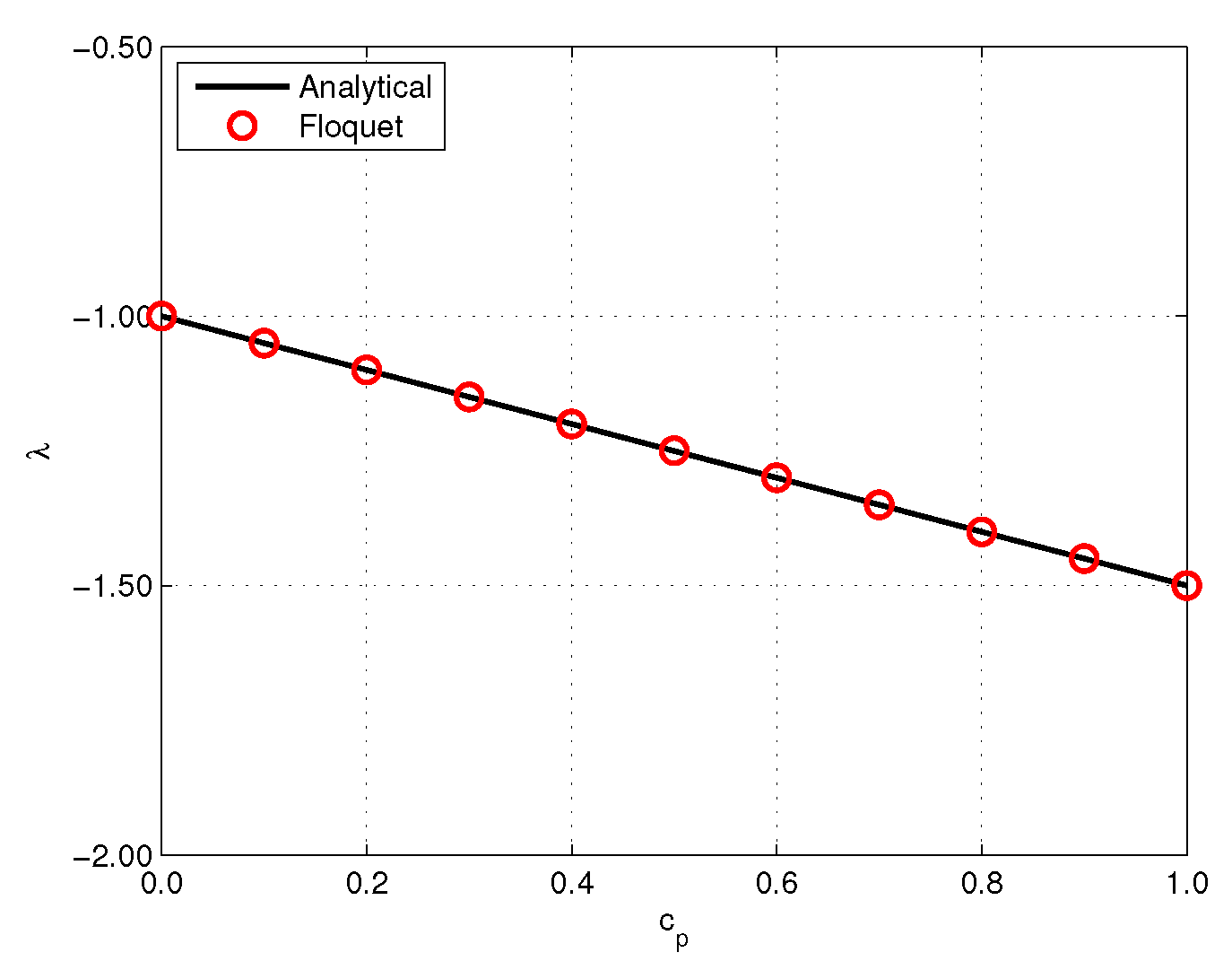
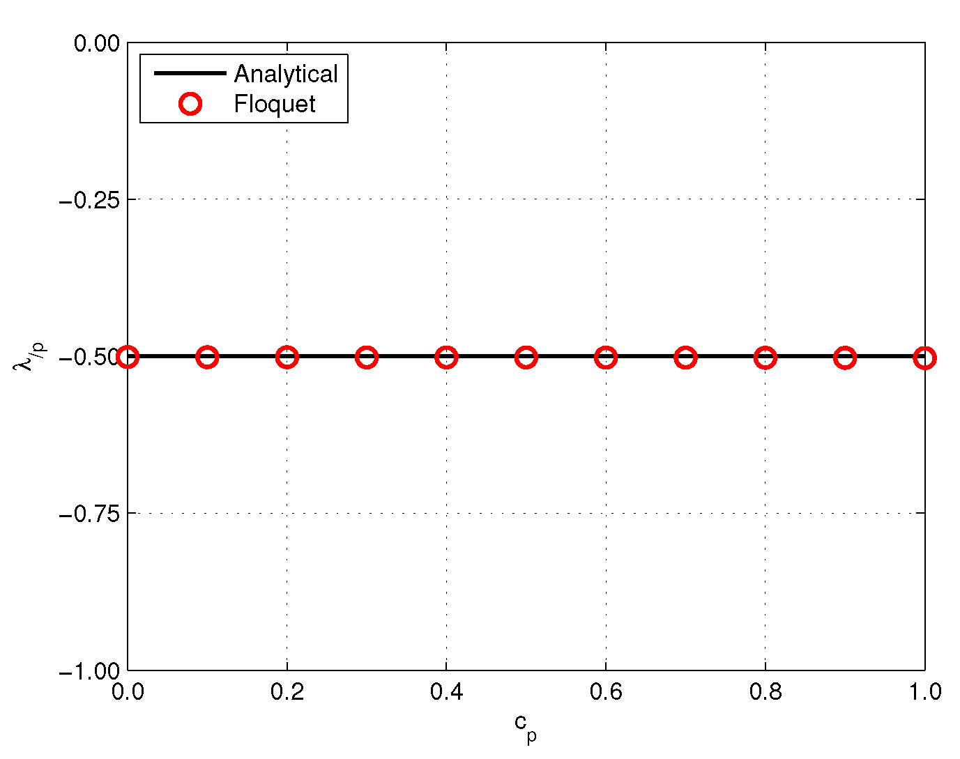
3.1. Verification with an Analytical Solution

Before providing the detailed rotorcraft model and its stability analysis using LCEs, the proposed procedure was verified against analytical solution. Consider the homogeneous mass-damper system with a periodic damping term:
m x ¨ + ( c 0 + c p cos 2 t ) x ˙ = 0 ,
where the system has a period of π radians. Then, the system can be considered as a first order system with q = x ˙ .
q ˙ = ( c 0 + c p cos 2 t ) m q = 0
The monodromy matrix (in this case a scalar) can be obtained by integrating Equation (40) from an initial time t = 0 to t = T . Let m = 1 ;
q T q 0 = H = e 0 T [ c 0 + c p cos 2 t ] d t = e T c 0 T 2 c p
The eigenvalue of the system λ can be obtained from the eigenvalue of the monodromy matrix:
λ = 1 T log ( H ) = 1 T log ( e T c 0 T 2 c p ) = c 0 1 2 c p
If the coefficient of the periodic term, c p , is considered as the parameter; the sensitivity of the eigenvalue, λ p , can be analytically obtained as:
λ / p = 1 2 .
The analytical results are compared with the LCE numerical solution for c 0 = c p = 1 . Figure 1 presents the characteristic exponent obtained by the analytical and numerical (named Floquet), and Figure 2 gives the corresponding sensitivity of the characteristic exponents. Results show good correlation.

3.2. Complex LTP Rotorcraft Model

The nature of rotary-wing stability presents the interaction of structural dynamics, aerodynamics, and control systems to model rotorcraft components, such as rotors, fuselage, gearbox, etc. Each component may require a considerable number of degrees of freedom to describe the problem within the desired accuracy, even in its simplest and most compact form. As discussed earlier in this paper, LCEs estimation requires matrix operations at each time-step, including multiplications and orthogonalizations. Theoretically, this procedure should be carried on for an infinite limit ( t ), and in practice till LCEs converge to a steady finite value, a criterion that may not be verifiable in a trivial manner. This may require significant computational cost, compared to other classical methods that are otherwise limited to LTI or LTP problems [12].
In problems described with a relatively large number of degrees of freedom, only extracting the most critical LCEs or the few largest ones closest to zero can help improve computation efficiency [23,24]. However, in a detailed rotorcraft model, many lightly damped LCEs may appear, especially when the aircraft’s rigid body motion and fuselage elastic degrees of freedoms are considered. It may be impossible to discern between lightly damped modes that are not going to jeopardize stability and modes that, despite being more damped in the reference configuration, will eventually turn unstable for some variations of the parameters of the problem. Therefore, within the scope of this work, even when applied to a detailed problem, the method needs to be verified for the whole spectrum.

3.2.1. Model Description

To illustrate the application of the proposed approach to a complex problem, an aeroelastic model of a rotorcraft was developed, based on data for the AS-330 PUMA helicopter as presented in Reference [25]. Its general characteristics are reported in Table 1. The solidity parameter is the ratio of the actual rotor area over the area of the disk,
Solidity = N b c π R ,
where N b is the number of blades, and c is the chord, whereas the Lock number expresses the ratio between the aerodynamic and the inertia moments about the flap hinge that are associated with the flapping motion of the blades,
Lock number = ρ a c R 4 I β ,
where ρ is the air density, a the slope of the lift coefficient curve (often approximated as a = 2 π according to thin airfoil theory), and I β the moment of inertia of the blade about the flap hinge. These parameters are used to nondimensionalize the dynamics and aeromechanics of the main rotor (see, for example, Reference [2]). The overall model comprises:
  • all six rigid body modes (Fore/Aft, Lateral, Plunge, Roll, Pitch, and Yaw);
  • flight mechanics derivatives of the fuselage determined by fuselage/wing-body, horizontal tail, and the vertical tail;
  • ten elastic airframe modes captured at airframe and connection locations (such as airframe rotor connection); additionally, 1.5 % modal damping was also added;
  • three bending modes of the rotor in multiblade coordinates, formulated using a linerazized finite volume approach [26];
  • three main rotor servo-actuators modelled as transfer function from the force applied by controls ( f c ) and requested displacement ( x c ) to the servoactuator displacement ( x s ), namely x s = H x x c + H f f c ;
  • lead-lag dampers for the main rotor blades.
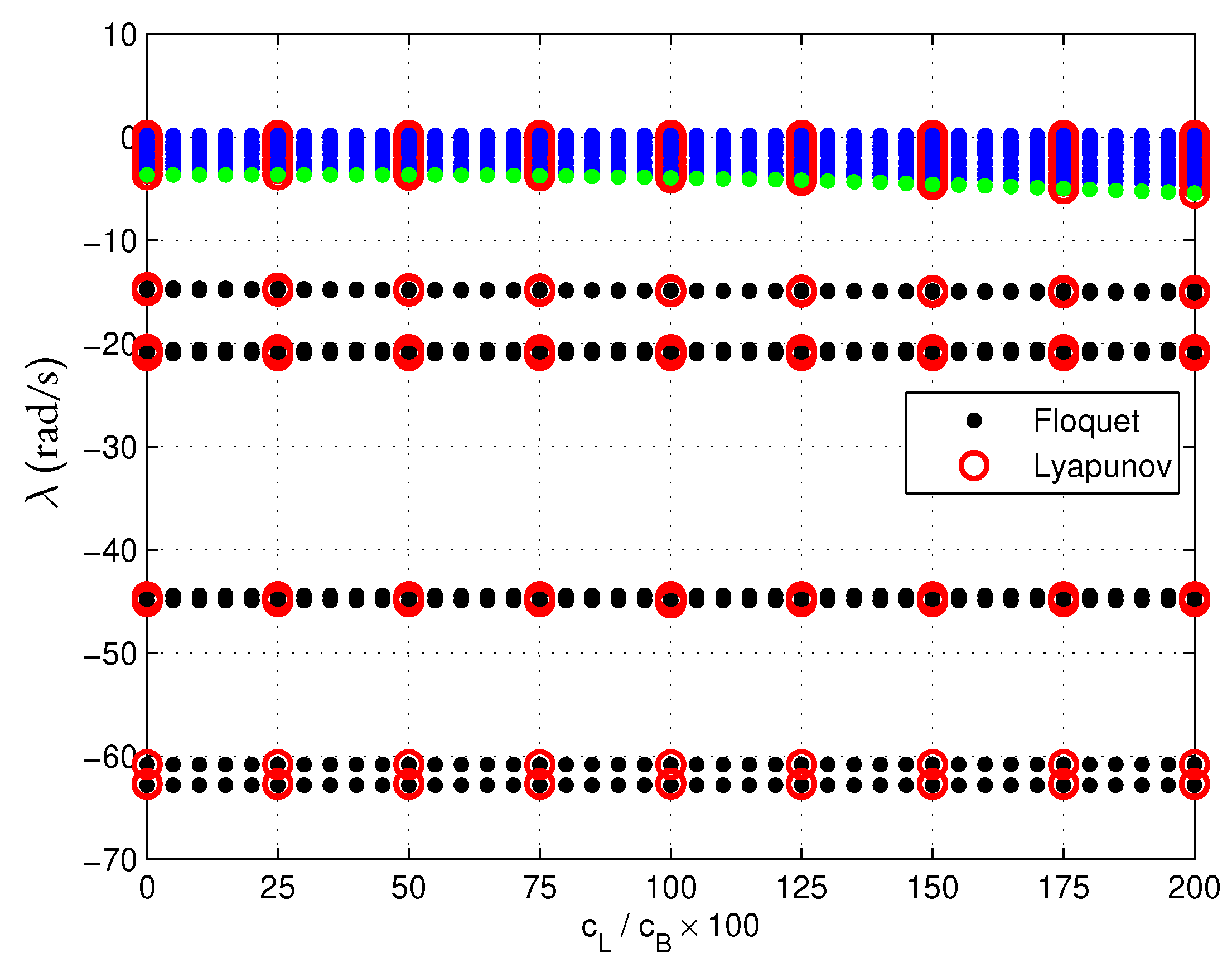
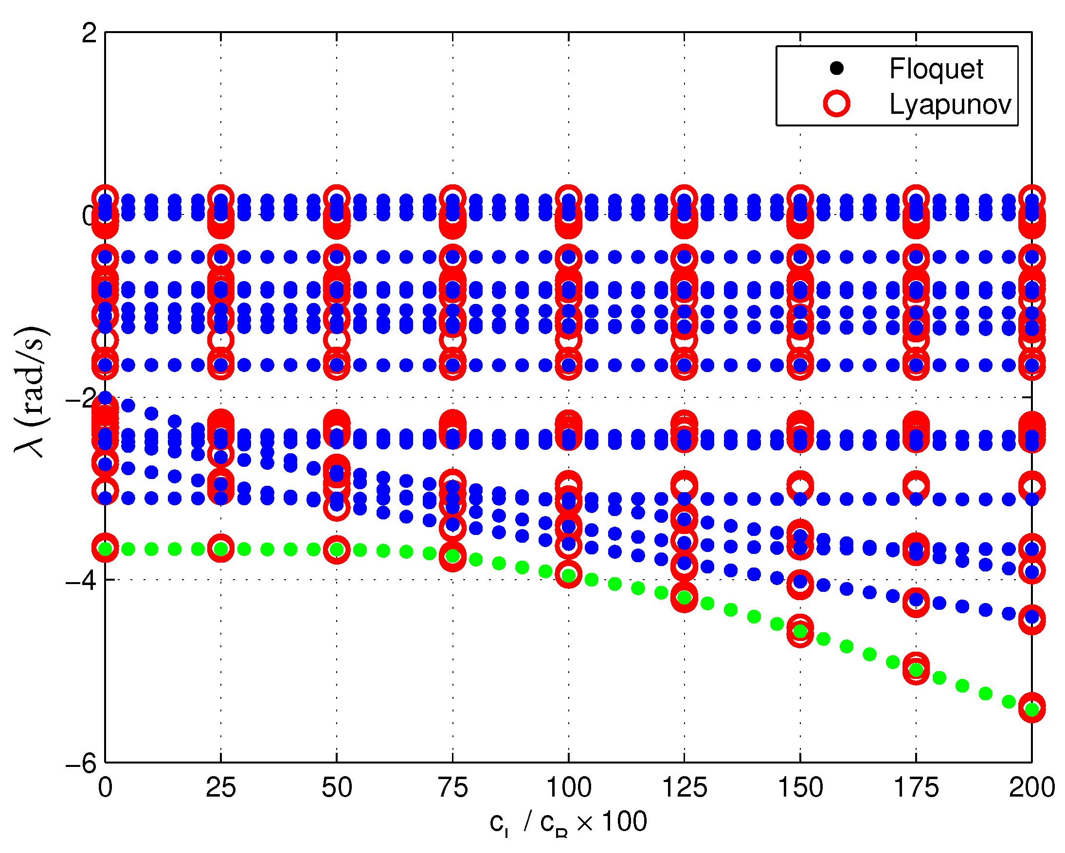
The above components are blended in MASST [27], an aeroservoelastic simulation platform with proven capabilities for rotorcraft comprehensive modeling [28,29]. The helicopter model is developed for hover flight, so the rotor model is isotropic; therefore, the model is linear time-invariant under normal conditions. Periodicity is introduced by considering the characteristic coefficient of the lead-lag damper of one blade as a parameter, varying from zero ( C L = 0 ) to twice its nominal value ( C L = 2 C d ), while the other dampers maintain their nominal value ( C L = C d ). The resulting overall system of equations can be stated as:
M x ¨ + C ( t , T ) x ˙ + K x = 0 ,
where T is the period of the system, namely reciprocal of the rotor angular speed T = 1 / Ω .
While the mass matrix M and stiffness matrix K are constant in time, the damping matrix C is periodic due to the asymetric distribution of lead-lag dampers. The resulting model is LTP with respect to the angular motion of the rotor. Stability and sensitivity analyses of the LTP model are performed using Lyapunov’s theory, as explained in a previous section. To illustrate the effectiveness of the proposed method, LCEs and their sensitivity are estimated and compared to that of the Floquet multipliers and their analytical sensitivities using the formulation in Ref. [30].

3.2.2. Analysis

Figure 3 presents the characteristic exponents resulting from both Floquet’s and Lyapunov’s analysis in the parameter range of interest. The LCEs show a good correlation with Floquet’s exponents. One can also observe that the higher modes (larger absolute valued LCEs) are not sensitive to the parameter change. However, some lightly damped modes that strongly interact with the in-plane motion of the rotor show higher sensitivity to the dissimilarity in the rotor blades’ dynamics. This can be better observed in Figure 4, which zooms on lightly damped modes.
Among the lightly damped modes, the one corresponding to regressive cyclic lag is the one that has the largest sensitivity to the parameter change. The corresponding LCEs and Floquet multipliers were separately plotted in Figure 5. It can be observed that the system does not lose the stability of the coupled airframe/lead-lag motion as one lead-lag damper reduces its effectiveness. Even when one damper is completely inoperative, the system is stable, which is most likely due to the presence of aerodynamic damping resulting from the coupled lag-flap motion.
The sensitivities corresponding to the LCEs and Floquet multipliers of Figure 5 are shown in Figure 6. Sensitivity estimates of the LCEs are compared with the corresponding sensitivity of the Floquet exponents and with analogous results obtained from numerical differentiation through finite differences. Results show that the sensitivity estimates obtained using LCEs are close enough to those obtained via finite differences, but not as close to those obtained through the sensitivity analysis of Floquet’s exponents.

4. Conclusions

This work presented the use of Lyapunov Characteristic Exponents (LCEs) for the estimation of the stability properties of time-dependent rotorcraft models. The theory of LCEs and the computation of their parameter sensitivity were presented with practical estimation methods. The proposed approach was applied to a comprehensive aeroelastic rotorcraft model. Time-variance was introduced by changing the properties of one of the lead-lag dampers, resulting in a time-periodic system. The resulting LCEs and their sensitivity were compared with those resulting from the Floquet method. The LCEs were in very good agreement with Floquet multipliers. Considering that the LCEs can also be generalized to non-linear problems, LCEs can represent a replacement and a generalization of the Floquet method. The analytical sensitivity estimation was not as successful, although found in relatively good agreement with finite-difference estimations. More efficient LCE sensitivity estimation algorithms are needed to improve that aspect of LCEs.

Author Contributions

Conceptualization, A.T. and P.M.; methodology, A.T. and P.M; software, A.T.; formal analysis, A.T.; investigation, A.T.; writing—original draft preparation, A.T.; writing—review and editing, A.T. and P.M.; visualization, A.T. All authors have read and agreed to the published version of the manuscript.

Funding

This research received no external funding. The APC was funded by Imperial College London Open Access Fund.

Institutional Review Board Statement

Not applicable.

Informed Consent Statement

Not applicable.

Conflicts of Interest

The authors declare no conflict of interest.

Abbreviations

The following abbreviations are used in this manuscript:
LCELyapunov Characteristic Exponents
LTILinear, Time-Invariant
LTPLinear, Time-Periodic
LTVLinear, Time-Variant
STMState Transition Matrix

References

  1. McGowen, S.S. Helicopters, an Illustrated History of Their Impact; ABC Clio: Santa Barbara, CA, USA, 2005. [Google Scholar]
  2. Johnson, W. Rotorcraft Aeromechanics; Cambridge University Press: New York, NY, USA, 2013. [Google Scholar]
  3. Filippone, A. Flight Performance of Fixed and Rotary Wing Aircraft; Elsevier: Amsterdam, The Netherlands, 2006. [Google Scholar]
  4. Anonymous. Rotorcraft Flying Handbook; FAA H-8083-21; Federal Aviation Administration: Washington, DC, USA, 2000. [Google Scholar]
  5. Ferrer, R.; Krysinski, T.; Auborg, P.; Belizzi, S. New Methods for Rotor Tracking and Balance Tuning and Defect Detection Applied to Eurocopter Products. In Proceedings of the American Helicopter Society 57th Annual Forum, Washington, DC, USA, 9–11 May 2001. [Google Scholar]
  6. Hammond, C.E. An Application of Floquet Theory to Prediction of Mechanical Instability. J. Am. Helicopter Soc. 1974, 19, 14–23. [Google Scholar] [CrossRef] [Green Version]
  7. Hirsch, M.W.; Smale, S.; Devaney, R.L. Differential Equations, Dynamical Systems, and an Introduction to Chaos; Elsevier: San Diego, CA, USA, 2004. [Google Scholar]
  8. Hull, D.G. Fundamentals of Airplane Flight Mechanics; Springer: Berlin/Heidelberg, Germany, 2007. [Google Scholar]
  9. Bittanti, S.; Colaneri, P. Periodic Systems: Filtering and Control; Springer: London, UK, 2009. [Google Scholar]
  10. Bielawa, R.L. Rotary Wing Structural Dynamics and Aeroelasticity, 2nd ed.; AIAA: Washington, DC, USA, 2005. [Google Scholar]
  11. Benettin, G.; Galgani, L.; Giorgilli, A.; Strelcyn, J.M. Lyapunov characteristic exponents for smooth dynamical systems and for Hamiltonian systems; a method for computing all of them. Part 1: Theory. Meccanica 1980, 15, 9–20. [Google Scholar] [CrossRef]
  12. Tamer, A.; Masarati, P. Stability of Nonlinear, Time-Dependent Rotorcraft Systems Using Lyapunov Characteristic Exponents. J. Am. Helicopter Soc. 2016, 61, 14–23. [Google Scholar] [CrossRef]
  13. Masarati, P.; Tamer, A. Sensitivity of trajectory stability estimated by Lyapunov characteristic exponents. Aerosp. Sci. Technol. 2015, 47, 501–510. [Google Scholar] [CrossRef] [Green Version]
  14. Adrianova, L.Y. Introduction to Linear Systems of Differential Equations. In Translations of Mathematical Monographs; American Mathematical Society: Providence, RI, USA, 1995; Volume 146. [Google Scholar]
  15. Medio, A.; Lines, M. Nonlinear Dynamics—A Primer; Cambridge University Press: Cambridge, MA, USA, 2001. [Google Scholar]
  16. Strogatz, S.H. Nonlinear Dynamics and Chaos: With Applications to Physics, Biology, Chemistry, and Engineering; Perseus Books: Reading, MA, USA, 1994. [Google Scholar]
  17. Hsu, C.S. On approximating a general linear periodic system. J. Math. Anal. Appl. 1974, 45, 234–251. [Google Scholar] [CrossRef] [Green Version]
  18. Friedmann, P.; Silverthorn, J. Aeroelastic Stability of Periodic Systems with Application to Rotor Blade Flutter. AIAA J. 1974, 12, 1559–1565. [Google Scholar] [CrossRef]
  19. Rao, S.S. Engineering Optimization; John Wiley & Sons: New York, NY, USA, 1996. [Google Scholar]
  20. Tamer, A.; Masarati, P. Sensitivity of Lyapunov Exponents in Design Optimization of Nonlinear Dampers. J. Comput. Nonlinear Dyn. 2019, 14, 021002. [Google Scholar] [CrossRef]
  21. Krauskopf, B.; Osinga, H.M.; Galán-Vioque, J. Numerical continuation methods for dynamical systems; Springer: Dordrecht, The Netherlands, 2007. [Google Scholar]
  22. Dieci, L.; Van Vleck, E.S. Lyapunov Spectral Intervals: Theory and Computation. SIAM J. Numer. Anal. 2002, 40, 516–542. [Google Scholar] [CrossRef]
  23. Rosenstein, M.T.; Collins, J.J.; De Luca, C.J. A practical method for calculating largest Lyapunov exponents from small data sets. Phys. D Nonlinear Phenom. 1993, 65, 117–134. [Google Scholar] [CrossRef]
  24. Fu, S.; Wang, Q. Estimating the largest Lyapunov exponent in a multibody system with dry friction by using chaos synchronization. Acta Mech. Sin. 2006, 22, 277–283. [Google Scholar] [CrossRef]
  25. Bousman, W.G.; Young, C.; Toulmay, F.; Gilbert, N.E.; Strawn, R.C.; Miller, J.V.; Maier, T.H.; Costes, M.; Beaumier, P. A Comparison of Lifting-Line and CFD Methods with Flight Test Data from a Research Puma Helicopter; TM 110421; NASA: Moffett Field, CA, USA, 1996. [Google Scholar]
  26. Tamer, A.; Masarati, P. Linearized structural dynamics model for the sensitivity analysis of helicopter rotor blades. In Proceedings of the Ankara International Aerospace Conference, Ankara, Turkey, 11–13 September 2013. [Google Scholar]
  27. Masarati, P.; Muscarello, V.; Quaranta, G. Linearized Aeroservoelastic Analysis of Rotary-Wing Aircraft. In Proceedings of the 36th European Rotorcraft Forum, Paris, France, 7–9 September 2010. [Google Scholar]
  28. Tamer, A.; Zanoni, A.; Cocco, A.; Masarati, P. A numerical study of vibration-induced instrument reading capability degradation in helicopter pilots. CEAS Aeronaut. J. 2014, 12, 427–440. [Google Scholar] [CrossRef]
  29. Tamer, A.; Muscarello, V.; Quaranta, G.; Masarati, P. Cabin Layout Optimization for Vibration Hazard Reduction in Helicopter Emergency Medical Service. Aerospace 2020, 7, 59. [Google Scholar] [CrossRef]
  30. Tamer, A.; Masarati, P. Periodic Stability and Sensitivity Analysis of Rotating Machinery. In Proceedings of the 9th IFToMM International Conference on Rotor Dynamics; Pennacchi, P., Ed.; Mechanisms and Machine Science; Springer: Cham, Switzerland, 2015; Volume 21. [Google Scholar] [CrossRef]
Figure 1. Comparison of the characteristic exponents obtained by analytical solution and numerical method (Floquet).
Aerospace 09 00010 g001
Figure 2. Comparison of the sensitivity characteristic exponents obtained by analytical solution and numerical method (Floquet).
Aerospace 09 00010 g002
Figure 3. Characteristic exponents estimated by Lyapunov theory (LCEs) and Floquet multipliers, whole range. The lightly damped modes are marked with blue.
Aerospace 09 00010 g003
Figure 4. Characteristic Exponents estimated by Lyapunov theory (LCEs) and Floquet multipliers, zoom of lightly damped modes from Figure 3. The lightly damped blade lead-lag mode is marked in green.
Aerospace 09 00010 g004
Figure 5. Characteristic exponents estimated by Lyapunov theory (LCEs) and Floquet multipliers, corresponding to the lightly damped blade lag mode, isolated and zoomed from Figure 4.
Aerospace 09 00010 g005
Figure 6. Sensitivity estimates of characteristic exponents from Lyapunov theory (LCEs), Floquet Analysis, and finite differences, corresponding to the lightly damped blade lag mode of Figure 5.
Aerospace 09 00010 g006
Table 1. AS-330 PUMA general characteristics [25].
ParameterValueUnits
Helicopter
Gross Weight7400kg
Max Speed140kn
Main Rotor
Number of blades4
Radius7.49m
Solidity0.0913(n.d.)
Lock number8.70(n.d.)
Speed270rpm
Flap frequency1.03/rev
Lag Frequency0.26/rev
Publisher’s Note: MDPI stays neutral with regard to jurisdictional claims in published maps and institutional affiliations.

