Abstract
Airport traffic flow prediction is a fundamental research topic in the field of air traffic flow management. Most existing works focus on the single airport traffic flow prediction with temporal dynamics but fail to consider the influence of the topological airport network. In this paper, a novel deep learning-based framework, called airport traffic flow prediction network (ATFPNet), is proposed to capture spatial-temporal dependencies of the historical airport traffic flow (departure and arrival) for the multiple-step situational (network-level) arrival flow prediction. Firstly, considering the nature of the airport distribution and the context of air transportation, a special semantic graph built on the flight schedule is applied to represent the airport network, which is the key to encoding the situational airport traffic flow into a single representation. Then, the graph convolution operator and the gated recurrent unit are combined to extract high-level transition patterns of airport traffic flow in the spatial and temporal dimensions. Finally, a real-world airport traffic flow dataset is applied to validate the effectiveness of the proposed model, and the experimental results demonstrate that the ATFPNet outperforms other baselines on different prediction horizons. Specifically, the proposed method achieves up to 17% MAE improvement compared to baselines. Based on the proposed approach, efficient traffic planning is expected to be achieved for airport management.
1. Introduction
With the spectacular increase of flights in air transportation, a large number of congestions and flight delays occur due to the limited airport capacity. Compared with the high cost of extending the airport infrastructure, enhancing the efficiency of the air traffic flow management (ATFM) at airports is a preferred option for concerned departments in short-term. As an essential technique in air traffic control (ATC), airport arrival flow prediction (AAFP) can detect the arrival demand timely, which is the foundation to provide decision-making on the ATFM. On the one hand, it helps air traffic controllers (ATCOs) to foresee real-time airspace situations at airports, relieving the workload of the controllers. On the other hand, it can provide more time to make an efficient flow plan for alleviating airport traffic congestions in time.
The short-term arrival flow prediction in an ATC system is typically based on the historical and current airport traffic flow information, including departure flow, arrival flow, and so forth, to estimate the arrival flow in the near future. With regard to the air traffic prediction task [1,2], it is commonly agreed that it is subject to the complex spatial–temporal dependencies of traffic data. Therefore, when forecasting the airport arrival flow, it is necessary to consider the spatial and temporal dependencies integrally:
- (1)
- Spatial dependencies: the evolution of the airport arrival flow relates to the topological structure of a given airport network. In air transportation, the flights commute between airports conforming to a flight schedule overall, which contains the departure time, flight routes, and arrival time at airports. Therefore, a semantic airport network can be constructed with this scheduling, which takes airports as nodes, the city-pairs as edges and the number of scheduled flights between airports as the weight values. Specifically, as illustrated in Figure 1, the red link represents that there are scheduled flights that can commute between airports. The wider the link is, the more scheduled flights it has between both ends. Focusing on the city-pair between Beijing and Shanghai (ZBAA-ZSSS), both airports have a large number of actual arrival flights, which demonstrates that more scheduled flights may bring the larger arrival flow, and validate the effect of the semantic airport network.
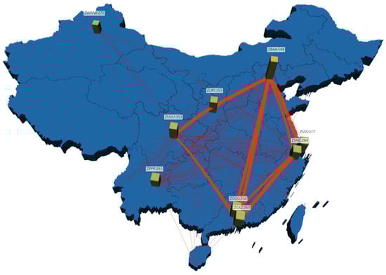 Figure 1. A simplified airport network. The top ten city-pairs according to the domestic scheduled flights are depicted by the wider red lines. The actual airport arrival flow is shown by the bar. The airport is identified by the four-letter location identifier code.
 - (2)
- Temporal dependencies: the airport arrival flow changes in periodicity, trend and closeness. As the flight operation is usually arranged by airlines weekly, the airport arrival flow presents periodical patterns each week. Within one day, the peak hours of the airport arrival flow usually surge during 12:00–14:00 and 17:00–19:00, and the bottom mostly appears between 00:00 and 07:00. The closeness means that the arrival flow on the adjacent time slice often changes smoothly.
For years, great efforts have been made to improve the performance of traffic flow prediction. In terms of prediction methods, the previously published works can generally be classified into three categories, that is, flight plan-based algorithms, traffic flow model-driven algorithms and data-driven algorithms. The flight plan-based algorithms achieve air traffic flow of the airspaces concerned by evaluating the 4-D aircraft trajectories [3] based on flight plans [4,5]. This method relies heavily on the trajectory prediction (TP) technique, which is susceptible to uncertainties of the real-time traffic state, such as the weather condition and the airport facility state. As a result, the flight plan-based approaches failed to offer sufficient insights into the dynamics of the traffic flow [6]. The flow model-driven algorithms generally learn the evolution pattern of the traffic flow by some handcrafted traffic models. Prior knowledge is required to design the traffic model to forecast future traffic flow, including the cell transmission model [7], the queuing theory model [8], and the aggregate flow model [9,10,11], and so forth. However, the traffic state is influenced by many factors so that it may be difficult to fully illustrate unsteady air traffic flow by a specific model. The core idea for data-driven algorithms is to extract informative knowledge by mining the input dataset. The history average model (HA) [12] is an early representative method. Recently, there is an increasing interest in applying methods based on Machine Learning Techniques (MLT) to problems in Air Traffic Management (ATM) [13]. Some neural network models were proposed to achieve the traffic prediction, including the artificial neural network (ANN) [14], the long short-term memory (LSTM) [15,16,17], the gated recurrent unit (GRU) [18] and the convolutional neural network (CNN) [19,20]. In general, the LSTM and the GRU models are able to provide a higher performance for time-series prediction tasks. However, as it fails to consider the spatial dependencies, the structure of the airport network is not captured in the related AAFP task. To capture the spatial dependencies of air traffic flow, the CNN model was used to mine the grid-based traffic flow by dividing the space into grided regions [2]. However, due to the graph nature of the airport network, it may not be an optimal solution to directly extract the underlying patterns of the topological structure of the airport network by the CNN.
As deep learning models have been particularly successful in dealing with speech [21,22,23], images [24,25,26,27], or videos [28], the increasing architectures based on the graph neural network were proposed to extract informative graph representations for subsequent tasks. The graph convolutional network (GCN) [29] is a generalized CNN, which can mine the high-level information in a non-Euclidean space directly. In addition, some integrated neural networks were also developed to mine the spatial-temporal data efficiently. The spectral graph Markov network (SGMN) [30] was proposed to approximately characterize the dynamic change of traffic data. However, the Markov assumption of the SGMN may limit its performance on the multiple-step prediction tasks.
To solve the aforementioned problems, we first represent the airport network as a weighted graph based on a flight schedule, generally describing the spatial interactions of flights between airports. In succession, an airport traffic flow prediction network (ATFPNet), constructed by the graph convolution operator and the gated recurrent unit, is proposed to capture the evolution patterns of the airport traffic flow. Specifically, the overall traffic flow in the airport network can be encoded into a single structure by the specific graph representation. Thanks to the recurrent mechanism of the ATFPNet cell, the proposed approach has the ability to predict the multiple-step airport arrival flow in a situational manner. In addition, a real-world airport traffic flow dataset is constructed to validate the proposed approach, and the results demonstrate that the proposal outperforms other baselines, achieving up to 17% MAE improvement. All in all, the main contributions of this paper are summarized as follows:
- Considering the air transportation context, a semantic airport network is built up by the flight schedule, which generally models the flights interactions between airports;
- In light of the semantic airport network, a deep learning-based ATFPNet framework is proposed to predict the airport arrival flow in a multiple-step and situational manner, which is able to consider the spatial-temporal dependencies of airport traffic flow integrally;
- The graph convolutional network and gated recurrent unit are combined to construct the ATFPNet model, which is the key to extracting the high-level transition patterns of airport traffic flow. Specifically, the spatial dependencies of inter-airports and the time-varying airport traffic flow sequence can be modeled by the two blocks, respectively;
- A real-world dataset from the Civil Aviation Administration of China (CAAC) is applied to evaluate the performance of the proposed approach. Compared to the other baselines, the experimental results demonstrate that the proposed approach yields performance superiority for the short-term situational airport arrival flow forecasting.
The rest of this paper is organized as follows. Implementation details of the proposed model are introduced in Section 2. In Section 3, we list experimental configurations and evaluate the experimental results by a real-world airport traffic flow dataset. The discussion of the experiment is reported in Section 4. We conclude the paper and introduce the future work in Section 5.
2. Methodologies
2.1. Airport Network Representation
The airport network is defined as an undirected graph , where V is a finite set of nodes, and E is a set of edges. is a weighted adjacent matrix of G, indicating the proximity between nodes on the network, where N is the number of nodes. Specifically, considering the operational characteristics of the air traffic, we make statistics of the scheduled flights between each airport pairs to present the weighted adjacent matrix A, where . The element is 0 if there is no scheduled flight between airports, and denotes the number of the scheduled flights.
2.2. Airport Arrival Flow Prediction Problem
The goal of the airport arrival flow prediction is to simultaneously predict network-level airport arrival flow by the current and historical airport traffic flow (departure and arrival). We regard the airport traffic flow as the attribute feature of the node on the network. The network-level features for multiple time steps can be characterized as an Equation (1):
in which demonstrates the traffic flow of N given airports at the n-th time step, is the length of the sequence , S represents the length of sum time steps (the length of all historical time series), and D denotes the dimension of a node feature. Therefore, the multiple-step situational airport arrival flow prediction can be termed as learning the mapping function on the premise of the airport network G and the feature matrix X. Thus, the next t steps AAFP task can be shown in Equation (2):
where the is a traffic flow prediction model that is usually optimized by data-driven methods. t is the length of the time series needed to be predicted. Notably, is the prediction results, which may have different dimensions with the input feature matrix X.
2.3. Airport Traffic Flow Prediction Network
To improve the accuracy of arrival flow prediction on the airport network, an airport traffic flow prediction network (ATFPNet) is proposed considering the spatial-temporal dependencies of the input features. The architecture of an ATFPNet cell is visualized in Figure 2. The left part is an ATFPNet cell with output and input at the t time instant. denotes the hidden state from the previous time step with vector components . The right part represents the components of an ATFPNet cell, which combines the spatial graph convolution (GC) block and the gated recurrent unit. The GC is a generalization of a convolution operator in the non-Euclidean space, which aggregates neighborhood information via a normalized Laplacian matrix without required eigen-decomposition. Therefore, the GC can process non-Euclidean data (like a graph) directly at a low computation cost. By stacking multiple convolutional layers, the complex spatial dependencies can be captured efficiently. For example, a two-layer GC block can be expressed as Equation (3):
where X denotes the feature matrix and A represents the adjacent matrix. is a transformation of A, where , and is a degree matrix describing the number of edges attached to each node, which can be obtained by . The parameters and represent the weighted matrix in the first and second layers, respectively, is the activation function. In this work, the structure of the airport network is represented as the adjacent matrix A.
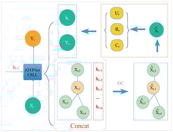
Figure 2.
The architecture of an ATFPNet cell.
In traffic prediction, the ability to mine the transition patterns from sequential data is indispensable for capturing the temporal dependencies. The recurrent neural network (RNN) is widely used to handle this task and showed the desired performance for different tasks. However, the RNN block suffers the problem of gradient vanishing and exploding, which limits the model convergence and the final performance. The LSTM and the GRU models were proposed to address the above issues by incorporating the gate mechanism into the RNN. Compared to the LSTM, the GRU is similarly effective with a simpler architecture [31]. Therefore, the GRU is selected as a basic block to capture temporal dependencies of the features, as shown below:
where the notation denotes the output at time instant , and are the update gate, reset gate at time instant t, respectively, and represent the learnable weights and deviations in the training process, and denotes the output at time instant t. Combining the GC block with the gated recurrent unit, the inference rules of the ATFPNet are shown in Equations (8)–(11).
where the represents the graph convolution process and A represents the adjacent matrix. The other notations in Equations (8)–(11) are the same as those in Equations (4)–(7). At a given time instant, the dynamic patterns of the airport traffic flow sequence can be learned by the AFTPNet cell. By unrolling the ATFPNet cells, the proposed model can capture informative features to predict the arrival flow. The process of ATFPNet for multiple-step situational prediction is described in Figure 3. Subgraph A is an example that demonstrates the process of unrolling ATFPNet cells, like that of the GRU cells. Subgraph B shows that the ATFPNet captures the topological relationship between the neighbors and adjacent time instants.
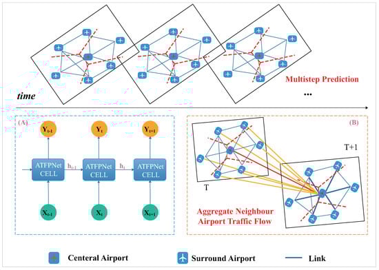
Figure 3.
The process of the ATFPNet for multiple-step situational prediction, which contains the process of unrolling the ATFPNet cells and the operation of aggregating features of the adjacent spatial-temporal nodes.
In summary, a dedicated weighted graph is applied to represent the airport network, considering the air traffic operation context (flight schedule). On the other hand, the GC block and gated recurrent unit are combined to capture the spatial-temporal dependencies of features integrally and finally achieve the multiple-step situational AAFP task.
3. Experiments
3.1. Data Description
3.1.1. Airport Traffic Flow Dataset
To validate the proposed ATFPNet framework, the departure and arrival flight data of 224 civil airports in China from 1 June 2017 to 30 June 2017, is collected as a raw flight information database for data extraction and analysis. This database involves about 0.21 million pieces of information on domestic flights, which include: (1) flight number: a code for an airline service consisting of a three-character airline designator and several digits; (2) aircraft type: a designator with a four-character alphanumeric code defined by the International Civil Aviation Organization (ICAO); (3) departure and arrival airport: both designators are described by using the four-letter location identifier such as the Beijing Capital International Airport is represented as ZBAA; (4) actual departure time and actual arrival time: both fields are stored in the Chinese Standard Time (CST) format; (5) status of flight: a property denotes whether the departure and arrival airport of a flight is in China. An example of the flight information from a real ATC system in China is listed in Table 1.

Table 1.
An example of the flight information.
By traversing the flight information records, each airport half-hourly actual departure and actual arrival aircraft are counted and gathered, forming an airport traffic flow dataset. To avoid sparsity, the civil airports are ranked according to the handling capacity, and a total of 60 top busy airports (e.g., ZBAA, ZPPP) are poured into the experimental dataset, which account for about 75% of the air traffic in China. An example of the dataset is demonstrated in Table 2, containing the start time, end time, actual departures, and actual arrivals at the airports every other 30 min.
Table 2.
An instance of the airport traffic flow dataset.
For better convergence, the variables in the dataset were mapped into [0, 1] by the min–max normalization as the following Equation (12):
where , X, and represent the normalized value, the original value, the maximum, and the minimum value in the dataset, respectively. Finally, there are 1440 records in this dataset, spanning from 1 June 2017 to 30 June 2017 with 30 min intervals.
3.1.2. Aiport Network Construction
Considering the air traffic operation context, about 0.27 million scheduled domestic flights are used to construct the airport network as a weighted graph, which macroscopically describes the flights interactions on the network. The number of nodes in the airport network is set to 60, which follows the airport traffic flow dataset. An example of domestic scheduling is shown in Table 3, which includes the flight number, aircraft type, day of the week, departure airport, scheduled arrival time, scheduled departure time, arrival airport. Specifically, the column, day of the week, ranges from 1 to 7 designating Monday to Sunday. In addition, the formats of other columns are the same as the flight information shown in Table 1. After traversing every record in the flight schedule, the sum of the scheduled departure and the arrival aircraft between each city-pair can be obtained. By statistics, the top ten city-pairs in the scheduling are listed in Table 4, where we can find that the difference of flights between the inbound and the outbound is small. The average relative difference is calculated by Equation (13), which is about 0.02%.
where is the relative difference value for measuring the difference of flights on both directions in city-pairs, represents the direction from left to right in the city-pair, is in the inverse direction, and n is the number of city-pairs.
Table 3.
An example of a flight schedule.
Table 4.
The top ten city-pairs in the flight schedule in June 2017.
Due to the relatively small difference, the large flights flow in each city-pair can be used to approximately express the interactions strength of air traffic between airports. Therefore, we define the airport network as an undirected weighted graph. By Equation (12), the flow of flights is normalized into [0, 1], which is further regarded as the final weight value of the edge between nodes on the airport network. The graph presentation of the airport network is intuitively visualized in Figure 4. The brighter color indicates a large amount of air traffic according to the flight schedule, and the darker ones are small.
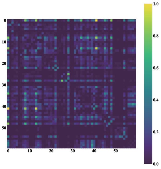
Figure 4.
The graph representation of the semantic airport network is built up by the flight schedule.
3.2. Evaluation Metrics
A total of three metrics are leveraged to evaluate the performance of the proposed ATFPNet, by measuring the difference between the real traffic information flow and the prediction flow , as shown below:
- RMSE
- MAE
- ACC
The RMSE and the MAE are the root mean square error and the mean absolute error, respectively. The ACC is used to detect the prediction performance. Specifically, as for the RMSE and MAE metrics, the smaller the value is, the better the prediction performance is, while the ACC presents an inverse trend.
3.3. Experiment Configurations
3.3.1. Training Details
In the experiment, we manually set the learning rate to 0.001, the batch size to 64 and the training epoch to 5000. As the airport arrival flow in the next two hours is preferred to make an ATC decision, the output length is set to 4 with 30-min as the interval. In addition, considering the long-distance flights in domestic China, the time span of the input feature sequence is set to 6 hours, namely, most of the O-D pairs in the domestic flight schedule can be accomplished during this period, and the destination airport arrival flow can be counted. Therefore, the length of the input time-series is set to 12. As a key parameter to deep learning models, the number of hidden units is selected by specific experiments to decide the optimal architecture, which is detailed in Section 3.4.1.
The ATFPNet framework is implemented using Python 3.7, and the deep learning models are constructed by the Pytorch 1.7.1 framework. The Adam optimizer is employed to optimize the model parameters during the training procedure. The configurations of the training server are listed as follows: an AMD Ryzen 2990WX CPU (3.00 GHz, 32 cores), 128 GB RAM, and two GPUs (GEFORCE RTX 2080 Ti, 11 GB memory).
3.3.2. Comparative Baselines
In this work, the following baseline models are also designed to further confirm the performance superiority of our proposed approach:
- HA [12]: The average value of each airport arrival flow with the week as the interval in the historical data (only the training dataset) is taken as the prediction results;
- ANN: The ANN is constructed with five hidden layers, with neurons of [128, 256, 512, 1024, 60], respectively. The initial learning rate is 1 × 10. In addition, the model is optimized by the MAE loss and the batch size is 32 during the training procedure;
- GRU [31]: The GRU is configured with one layer and 512 hidden units. The initial learning rate is 1 × 10. The model is trained with batch size 32 and loss function MAE;
- GCN [29]: A two-layer GCN is employed in this experiment. The initial learning rate is 1 × 10. The model is trained with batch size 32 and loss function MAE;
- ATFPNet: the ATFPNet network is introduced in detail in Section 2.3.
To underline the fair comparison of the network-level flow prediction performance, the baselines share the same dataset (training and validation), and the unified size of the input and output as the ATFPNet.
3.4. Experimental Results
3.4.1. The Number of Hidden Units in ATFPNet
In this section, we mainly focus on testing the optimal network architecture for the prediction performance of the ATFPNet. The hidden units of the GRU block are set to [16, 32, 64, 100, 128]. The experiment results of the ATFP task are shown in Figure 5, in which the horizontal and vertical axes denote the number of hidden units and different metrics, respectively. It can be seen that the evaluation metrics of the proposed model show the same trend in MAE and RMSE with increasing the hidden units. Specifically, the MAE and the RMSE firstly increase then decrease whereas the ACC is the opposite. When the number of hidden units increases to 64, the prediction precision is the maximum. As a result, it can be concluded that the 64 hidden units are the optimal choice for the prediction task in this work.
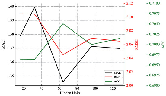
Figure 5.
The comparison of predicted performance under different hidden units in the ATFPNet.
3.4.2. Comparative Results with Existing Approaches
The experimental results are listed in Table 5, in which the ATFPNet and other baselines for different prediction horizons (from 30 to 120 min) are reported. From the results, it can be found that the proposed approach achieves the best performance. Specifically, compared with the baselines, with the increase of the prediction horizon, the ATFPNet obtains relative improvements on the MAE from 0.8% to 17%, the RMSE from 0.76% to 10.6%, and the ACC from 1.3% to 5.8%, respectively.
Table 5.
The prediction results of the ATFPNet and other baseline methods on the real-world airport traffic flow dataset from the CAAC.
Furthermore, the following conclusions can also be obtained from the experimental results:
- In general, the neural network-based methods achieve a better performance than the HA approach on all the prediction horizons. For the 30-min prediction horizon, compared to the HA, the RMSE and the MAE obtained by the neural network-based methods decrease by over 3.7% and 10.48%, respectively. From the perspective of air traffic data, the HA approach fails to handle the complex nonstationary network-level patterns of the time series data.
- For the neural network approaches, the prediction performance of the ANN approach is inferior to the others. The vanilla ANN fails to implement explicit spatial and temporal modeling for the input features, which limits the model convergence and the final performance. The GRU and the GCN baselines explicitly focus on the temporal and the spatial modeling of the airport traffic flow, respectively, which obtain a better performance compared to the ANN model. Specifically, compared to the GCN, the GRU model yields better evaluation metrics due to the temporal essence of the traffic flow.
- As can be seen from the experimental results, except for the HA approach, the prediction performance on all three metrics gradually degrades with the increase of the prediction horizon (from 30 to 120 min). The results can be attributed to the HA approach being a stationary approach that calculates the predicted value by averaging historical inputs, that is, independent of the prediction horizon. The data-driven baselines obtain better performance since they are able to leverage the input sequence to learn the complex transition patterns. Compared to the GCN model, the GRU and the proposed approach obtain a better performance, which confirms the contribution of the temporal modeling for the multiple-step prediction task (long-term temporal dependencies). Most importantly, by considering the desired temporal and spatial modeling, the proposed approach achieves a higher performance than GRU for the multiple-step prediction task. Specifically, the RMSE of ATFPNet is reduced from 0.7% to 2.1%, the MAE from 0.8% to 2.6%, respectively.
- Among the listed baselines, both the GCN and ATFPNet explicitly consider the spatial dependencies of the airport network to predict the airport arrival flow. The RMSE of the GCN models is reduced by approximately from 2.2% to 2.9%, and the MAE is improved from approximately 1.9% to 3.1% compared with the ANN model. In contrast to GCN (fails to achieve the temporal modeling), the RMSE of the ATFPNet is approximately reduced from 3.2% to 5%, and the MAE is approximately reduced from 4.4% to 7%. The experimental results show that both the temporal and spatial dependencies make significant contributions to the airport arrival flow prediction, which is the inspiration of the proposed approach.
4. Discussion
To further understand the proposed ATFPNet model, the Beijing international airport (i.e., ZBAA) was selected to visualize the prediction results. The results with the prediction horizons of 30-min, 60-min, 90-min, and 120-min are shown in Figure 6, Figure 7, Figure 8 and Figure 9, respectively. From the results, we can obtain the following conclusions:
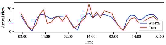
Figure 6.
The prediction results of the 30-min horizon.
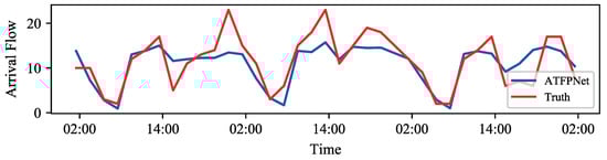
Figure 7.
The prediction results of the 60-min horizon.
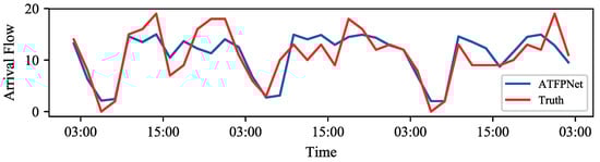
Figure 8.
The prediction results of the 90-min horizon.
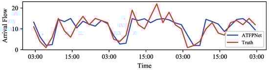
Figure 9.
The prediction results of the 120-min horizon.
- The prediction error for peaking hours is generally larger than that of other operation times, which can illustrate that the spatial graph convolution (a smooth filter) in the ATFPNet prefers to predict smaller changes. In addition, no flights operate in some branch airports for certain hours, in which the sparse inputs cause a smoother prediction.
- The prediction performance of the ATFPNet gradually decreases with the increase of the prediction horizon. It can be attributed that the transition patterns of airport arrival flow present higher non-linearity for a larger time window. The complexity of the airport arrival flow increases dramatically, which further limits the model performance.
- The ATFPNet can capture relatively long-term temporal dependencies among historical time slices. For example, as shown in Figure 9, when extending the interval to the 120-min, the ATFPNet always can detect a variation trend of the arrival flow at the given airport.
Although the performance is reduced for a larger prediction horizon, the proposed ATFPNet still outperforms other baselines. Specifically, the performance for predicting the 120-min horizon obtained by the ATFPNet is even better than that of the predicting the 30-min horizon obtained by the GCN baseline. The results demonstrate that considering both the spatial and temporal correlations can make the prediction model achieve the desired performance.
5. Conclusions
In this paper, we construct a deep-learning-based model, called the airport traffic flow prediction network (ATFPNet), to achieve the airport arrival flow prediction task. The spatial graph convolution operator and gated recurrent unit are combined to capture the transition patterns of airport traffic flow (departure and arrival). With respect to the air transportation context, a specific graph representation is built based on the flight schedule to illustrate the airport network. By further applying the GRU in the ATFPNet cell, the situational (network-level) multiple-step arrival flow can be achieved on the airport network. A real-world airport traffic dataset is applied to validate the proposed approach, and the experimental results show the performance superiority over other comparative baselines, concerning several data-driven models. Compared to the GRU model, the RMSE of ATFPNet is relatively improved from 0.7% to 2.1%. As for the GCN, the proposed approach obtains a better performance, reducing the RMSE from 3.2% to 5%. In summary, the airport network representation built on the flight schedule makes a great contribution to the situational airport arrival flow prediction task, and the proposed ATFPNet has the ability to capture the spatial and temporal features of airport traffic data.
In the future, except for the airport departure and arrival factors used in this paper, we plan to explicitly consider other factors to improve prediction accuracy, for example, weather information (visibility or thunderstorm), air traffic control information, the influence of international flights, and dynamic traffic movements on the network.
Author Contributions
Conceptualization, Z.Y. and Y.L.; Methodology, Y.L., H.Y. and Z.Y.; Software, Z.Y.; Formal analysis, Z.Y.; Writing—original draft preparation, Z.Y. and Y.L.; Writing—review and editing, Z.Y., F.L. and Y.L.; Visualization, Z.Y. All authors have read and agreed to the published version of the manuscript.
Funding
This work was supported by the National Natural Science Foundation of China (No. U20A20161), and the Open Fund of Key Laboratory of Flight Techniques and Flight Safety, CAAC (No. FZ2021KF04).
Institutional Review Board Statement
Not applicable.
Informed Consent Statement
Not applicable.
Data Availability Statement
Not applicable.
Conflicts of Interest
The authors declare no conflict of interest. The funders had no role in the design of the study; in the collection, analyses, or interpretation of data; in the writing of the manuscript, or in the decision to publish the results.
Abbreviations
The following abbreviations are used in this manuscript:
| ATC | Air Traffic Control |
| ATCOs | Air Traffic Controllers |
| ATFP | Air Traffic Flow Prediction |
| AAFP | Airport Arrival Flow Prediction |
| ATFM | Air Traffic Flow Control |
| ATM | Air Traffic Management |
| ATFPNet | Airport Traffic Flow Prediction Network |
| CAAC | Civil Aviation Administration of China |
| MLT | Machine Learning Techniques |
| CNN | Convolutional Neural Network |
| ANN | Artificial Neural Network |
| LSTM | Long Short-Term Memory |
| GRU | Gated Recurrent Unit |
| HA | Historical Average |
| TP | Trajectories Prediction |
| GCN | Graph Convolutional Network |
| SGMN | Spectral Graph Markov Network |
| GC | Graph Convlution |
| ACC | Accuracy |
| MAE | Mean Absolute Error |
| RMSE | Root Mean Squared Error |
| O-D | Origin and Destination |
| CST | Chinese Standard Time |
| ICAO | International Civil Aviation Organization |
References
- Liu, H.; Lin, Y.; Chen, Z.; Guo, D.; Zhang, J.; Jing, H. Research on the Air Traffic Flow Prediction Using a Deep Learning Approach. IEEE Access 2019, 7, 148019–148030. [Google Scholar] [CrossRef]
- Lin, Y.; Zhang, J.W.; Liu, H. Deep learning based short-term air traffic flow prediction considering temporal–spatial correlation. Aerospace Sci. Technol. 2019, 93, 105113. [Google Scholar] [CrossRef]
- Lin, Y.; Zhang, J.W.; Liu, H. An algorithm for trajectory prediction of flight plan based on relative motion between positions. Front. Inform. Technol. Electron. Eng. 2018, 19, 905–916. [Google Scholar] [CrossRef]
- Gong, C. A Methodology for Automated Trajectory Prediction Analysis. In Proceedings of the AIAA Guidance, Navigation, and Control Conference and Exhibit, Providence, RI, USA, 16–19 August 2004. [Google Scholar] [CrossRef]
- Lymperopoulos, I.; Lygeros, J.; Lecchini, A. Model Based Aircraft Trajectory Prediction During Takeoff. In Proceedings of the AIAA Guidance, Navigation, and Control Conference and Exhibit, Keystone, CO, USA, 21–24 August 2006. [Google Scholar] [CrossRef]
- Chengyuan, Z.; Xiao, B. Several Models of Air Traffic Flow. In Proceedings of the 2010 International Conference on E-Product E-Service and E-Entertainment, Henan, China, 7–9 November 2010. [Google Scholar] [CrossRef]
- Daganzo, C. On the Variational Theory of Traffic Flow: Well-Posedness, Duality and Applications. Netw. Heterog. Media 2006, 1, 601–619. [Google Scholar] [CrossRef]
- Mukherjee, A.; Lovell, D.; Ball, M.; Smith, R.; Odoni, A. Modeling Delays and Cancellation Probabilities to Support Strategic Simulations. In Proceedings of the 6th Europe-USA ATM Seminar, Baltimore, MD, USA, 27–30 June 2005; pp. 1–10. [Google Scholar]
- Sridhar, B.; Chatterji, G.; Sheth, K.; Soni, T. An Aggregate Flow Model for Air Traffic Management. J. Guid. Control Dyn. 2006, 29, 992–997. [Google Scholar] [CrossRef]
- Sridhar, B.; Chen, N.; Ng, H. An Aggregate Sector Flow Model for Air Traffic Demand Forecasting. In Proceedings of the 9th AIAA Aviation Technology, Integration, and Operations Conference (ATIO), Hilton Head, SC, USA, 21–23 September 2009. [Google Scholar] [CrossRef] [Green Version]
- Chen, D.; Hu, M.; Ma, Y.; Yin, J. A network-based dynamic air traffic flow model for short-term en route traffic prediction: Short-Term En Route Traffic Prediction. J. Adv. Transp. 2017, 50, 2174–2192. [Google Scholar] [CrossRef]
- Wei, G. A summary of traffic flow forecasting methods. J. Highw. Transp. Res. Dev. 2004, 21, 82–85. [Google Scholar]
- Sridhar, B.; Chatterji, G.B.; Evans, A.D. Lessons Learned in the Application of Machine Learning Techniques to Air Traffic Management; American Institute of Aeronautics and Astronautics: Reston, VA, USA, 2020. [Google Scholar] [CrossRef]
- Cheng, T.; Cui, D.; Cheng, P. Data mining for air traffic flow forecasting: A hybrid model of neural network and statistical analysis. In Proceedings of the 2003 IEEE International Conference on Intelligent Transportation Systems, Shanghai, China, 12–15 October 2003; Volume 1, pp. 211–215. [Google Scholar] [CrossRef]
- Fu, R.; Zhang, Z.; Li, L. Using LSTM and GRU neural network methods for traffic flow prediction. In Proceedings of the 2016 31st Youth Academic Annual Conference of Chinese Association of Automation (YAC), Wuhan, China, 11–13 November 2016; pp. 324–328. [Google Scholar] [CrossRef]
- Yang, Z.; Wang, Y.; Li, J.; Liu, L.; Ma, J.; Zhong, Y. Airport Arrival Flow Prediction considering Meteorological Factors Based on Deep-Learning Methods. Complexity 2020, 2020, 1–11. [Google Scholar] [CrossRef]
- Wei, G.; Wang, Z. Short-term airport traffic flow prediction based on lstm recurrent neural network. J. Aeronaut. Astronaut. Aviat. Ser. A 2017, 49, 299–307. [Google Scholar] [CrossRef]
- Zhang, D.; Kabuka, M.R. Combining weather condition data to predict traffic flow: A GRU-based deep learning approach. IET Intell. Transp. Syst. 2018, 12, 578–585. [Google Scholar] [CrossRef]
- He, K.; Zhang, X.; Ren, S.; Sun, J. Spatial Pyramid Pooling in Deep Convolutional Networks for Visual Recognition. IEEE Trans. Pattern Anal. Mach. Intell. 2015, 37, 1904–1916. [Google Scholar] [CrossRef] [PubMed] [Green Version]
- Li, Z.; Chen, G.; Zhang, T. A CNN-Transformer Hybrid Approach for Crop Classification Using Multitemporal Multisensor Images. IEEE J. Sel. Top. Appl. Earth Obs. Remote Sens. 2020, 13, 847–858. [Google Scholar] [CrossRef]
- Lin, Y.; Deng, L.; Chen, Z.; Wu, X.; Zhang, J.; Yang, B. A Real-Time ATC Safety Monitoring Framework Using a Deep Learning Approach. IEEE Trans. Intell. Transp. Syst. 2019, 21, 4572–4581. [Google Scholar] [CrossRef]
- Lin, Y.; Guo, D.; Zhang, J.; Chen, Z.; Yang, B. A Unified Framework for Multilingual Speech Recognition in Air Traffic Control Systems. IEEE Trans. Neural Netw. Learn. Syst. 2020, 32, 3608–3620. [Google Scholar] [CrossRef] [PubMed]
- Lin, Y.; Tan, X.; Yang, B.; Yang, K.; Zhang, J.; Yu, J. Real-time Controlling Dynamics Sensing in Air Traffic System. Sensors 2019, 19, 679. [Google Scholar] [CrossRef] [PubMed] [Green Version]
- Szegedy, C.; Liu, W.; Jia, Y.; Sermanet, P.; Reed, S.; Anguelov, D.; Erhan, D.; Vanhoucke, V.; Rabinovich, A. Going deeper with convolutions. In Proceedings of the 2015 IEEE Conference on Computer Vision and Pattern Recognition (CVPR), Boston, MA, USA, 7–12 June 2015; pp. 1–9. [Google Scholar] [CrossRef] [Green Version]
- Jiang, N.; Wang, K.; Peng, X.; Yu, X.; Wang, Q.; Xing, J.; Li, G.; Zhao, J.; Guo, G.; Han, Z. Anti-UAV: A Large Multi-Modal Benchmark for UAV Tracking. arXiv 2021, arXiv:2101.08466. [Google Scholar]
- Yu, X.; Gong, Y.; Jiang, N.; Ye, Q.; Han, Z. Scale Match for Tiny Person Detection. In Proceedings of the 2020 IEEE Winter Conference on Applications of Computer Vision (WACV), Snowmass Village, CO, USA, 1–5 March 2020; pp. 1246–1254. [Google Scholar] [CrossRef]
- Deng, L.; Gong, Y.; Lu, X.; Lin, Y.; Ma, Z.; Xie, M. STELA: A Real-Time Scene Text Detector with Learned Anchor. IEEE Access 2019, 7, 153400–153407. [Google Scholar] [CrossRef]
- Deng, H.; Hua, Y.; Song, T.; Zhang, Z.; Xue, Z.; Ma, R.; Robertson, N.; Guan, H. Object Guided External Memory Network for Video Object Detection. In Proceedings of the 2019 IEEE/CVF International Conference on Computer Vision (ICCV), Seoul, Korea, 27–28 October 2019; pp. 6677–6686. [Google Scholar] [CrossRef]
- Kipf, T.N.; Welling, M. Semi-Supervised Classification with Graph Convolutional Networks. arXiv 2016, arXiv:1609.02907. [Google Scholar]
- Cui, Z.; Lin, L.; Pu, Z.; Wang, Y. Transportation Research Part C-Graph Markov network for traffic forecasting with missing data. Transp. Res. Part C Emerg. Technol. 2020, 117, 102671. [Google Scholar] [CrossRef]
- Chung, J.; Gulcehre, C.; Cho, K.; Bengio, Y. Empirical Evaluation of Gated Recurrent Neural Networks on Sequence Modeling. arXiv 2014, arXiv:1412.3555. [Google Scholar]
Publisher’s Note: MDPI stays neutral with regard to jurisdictional claims in published maps and institutional affiliations. |
© 2021 by the authors. Licensee MDPI, Basel, Switzerland. This article is an open access article distributed under the terms and conditions of the Creative Commons Attribution (CC BY) license (https://creativecommons.org/licenses/by/4.0/).