Article

A Continuous Multivariable Finite-Time Super-Twisting Attitude and Rate Controller for Improved Rotorcraft Handling

Institute of Helicopter Technology, Department of Aerospace and Geodesy, Technical University of Munich, Boltzmannstr. 15, 85748 Garching, Germany
*
Author to whom correspondence should be addressed.
Aerospace 2022, 9(1), 6; https://doi.org/10.3390/aerospace9010006
Submission received: 27 October 2021 / Revised: 18 December 2021 / Accepted: 19 December 2021 / Published: 22 December 2021
(This article belongs to the Special Issue Rotorcraft)

Abstract

:
This paper synthesizes a continuous, multivariable, finite-time-convergent, super-twisting attitude and rate controller for rotorcraft with the objective of providing desired handling qualities and robustness characteristics. A sliding manifold is defined in the system state space to represent ideal attitude and rate command response dynamics of relative degree one with respect to the command input. Subsequently, robust command tracking is achieved via the synthesis of a multivariable super-twisting flight controller, which renders the plant states convergent on to the defined sliding manifold in finite-time and in the presence of matched external disturbance input. To validate the efficacy of the controller, simulation results are presented based on a nonlinear, higher-order rotorcraft model operating in turbulence. True system convergence to the sliding manifold from an untrimmed state is shown to lie within the theoretically predicted finite-time convergence bound. Furthermore, simulations with a linear quadratic flight controller are also presented for performance comparison with the proposed super-twisting flight controller.

1. Introduction

There is renewed interest in both manned and unmanned rotorcraft. Advances in electric/hybrid propulsion have led to a surge of new vertical take-off and landing (VTOL) prototypes aimed at commercial passenger operations. The diversity among eVTOL aircraft configurations is noteworthy, with designs ranging from vectored thrust to fixed multicopters, along with single person configurations such as hover bikes and personal flying devices (See evtol.news/aircraft (accessed on 27 October 2021) for an exhaustive list and References[1,2]). Likewise, unmanned rotorcraft are increasingly used in aerial logistics and allied missions (See recent statistics for unmanned aircraft systems in the United States: www.faa.gov/uas/resources/bythenumbers/ (accessed on 27 October 2021)).In the context of military missions, future high-speed VTOL aircraft are expected to impose new flight dynamic response requirements in the high-speed regime [3], representing a significant evolution and departure from conventional helicopter handling qualities requirements [4]. However, design complexities in conventional and unconventional rotorcraft continue to pose challenges, namely several degrees of freedom, higher-order dynamics, instability, complex aerodynamics, and the difficulty to fully characterize the entire spectrum of flight dynamic responses (see References [5,6] for a detailed discussion on the modeling and control challenges of conventional helicopters). As a result, flight dynamic models employed for controller synthesis in both conventional and unconventional configurations inherently include varying levels of uncertainty that cannot be fully characterized. These challenges will have to be overcome through innovative solutions to simplify piloting tasks and enable safe autonomous flight.
A robust controller capable of assuring specified performance under endogenous and exogenous uncertainty is likely to be an indispensable building block on which simplified manned missions and autonomous unmanned missions will hinge. For instance, References [1,2] reported in their experiments that very few “flight-naïve” test subjects they examined could safely translate an unaugmented VTOL personal aerial vehicle; only about half of them could use an attitude and rate command system, while a majority of them required a translational rate command system. Likewise, Reference [7] showed that inexperienced pilots could only fly a conventional helicopter when it was augmented via their H and μ controllers to offer translational rate command responses. Reference [8] showed the ability of a robust sliding mode flight controller to alleviate pilot workload for a shipboard landing task.
On the unmanned front, Reference [9] showed how a nonsingular terminal sliding mode controller and a disturbance observer could permit shipboard recovery of a small unmanned helicopter. Reference [10] flight-tested various unmanned rotorcraft maneuvers such as sling load and collision avoidance under atmospheric disturbance using a robust model predictive control scheme. Reference [11] gives a detailed survey of various control architectures developed for small unmanned helicopters, including robust control based.
Sliding mode control (SMC) is a promising robust control technique that can assure uniform, lower-order flight dynamic responses under uncertainty. SMC allows the designer to choose a sliding manifold representing reduced-order dynamics in the system’s state space. Conventional SMC techniques utilize a high frequency (theoretically infinite frequency) switching control action to force the system states to converge on the sliding manifold in finite time. Upon convergence, the same SMC control action continues to keep the system states on the sliding manifold by compensating for any matched uncertainty affecting the system [12]. However, such a controller becomes impractical to implement since theoretically infinite switching frequency is impossible to achieve by mechanical actuators. Applying finite switching control or the presence of unmodeled dynamics induces oscillations and limit-cycle behavior in the closed-loop system responses. This phenomenon is called as the “chattering effect” in the literature. Early approaches to alleviate chattering have adopted a continuous control approximation using the boundary layer concept, wherein a linear control approximation to the nonlinear switching control is applied inside a sufficiently small boundary about the sliding manifold, whereas the nonlinear switching control is applied outside of this boundary. Such a pseudo-SMC approach, however, degrades the desirable robustness properties of the original SMC, since the linear approximation inside the boundary layer is no longer completely robust to uncertainties [13]. Pseudo-sliding mode controllers based on the boundary layer concept have been developed and studied for rotorcraft flight control applications with good results in References [8,14,15,16,17,18].
Chattering alleviation by means of second order sliding mode (SOSM) controllers is an area of active research. The SOSM approach offers a continuous control signal (instead of a discontinuous one) without compromising the robustness properties of SMC [19]. One of the first SOSM helicopter flight controllers in Reference [20] showed robustness to both matched and unmatched perturbations. However, its design assumed input decoupling in an essentially highly-coupled, multi-input, multi-output plant, and it necessitated an observer to estimate the sliding variable derivative. A special case of SOSM is the super-twisting algorithm (STA) for systems of relative degree one [21]. Not only does STA obviate the need to estimate the sliding variable derivative but it also attenuates chattering, since the switching action appears under an integral. Recent results have extended the scalar super-twisting structure to a multivariable structure suitable for multi-input, multi-output, coupled systems [22,23], along with theoretical convergence time estimates [23].
On this background, the intent and contributions of this paper can be summarized as follows:
1.
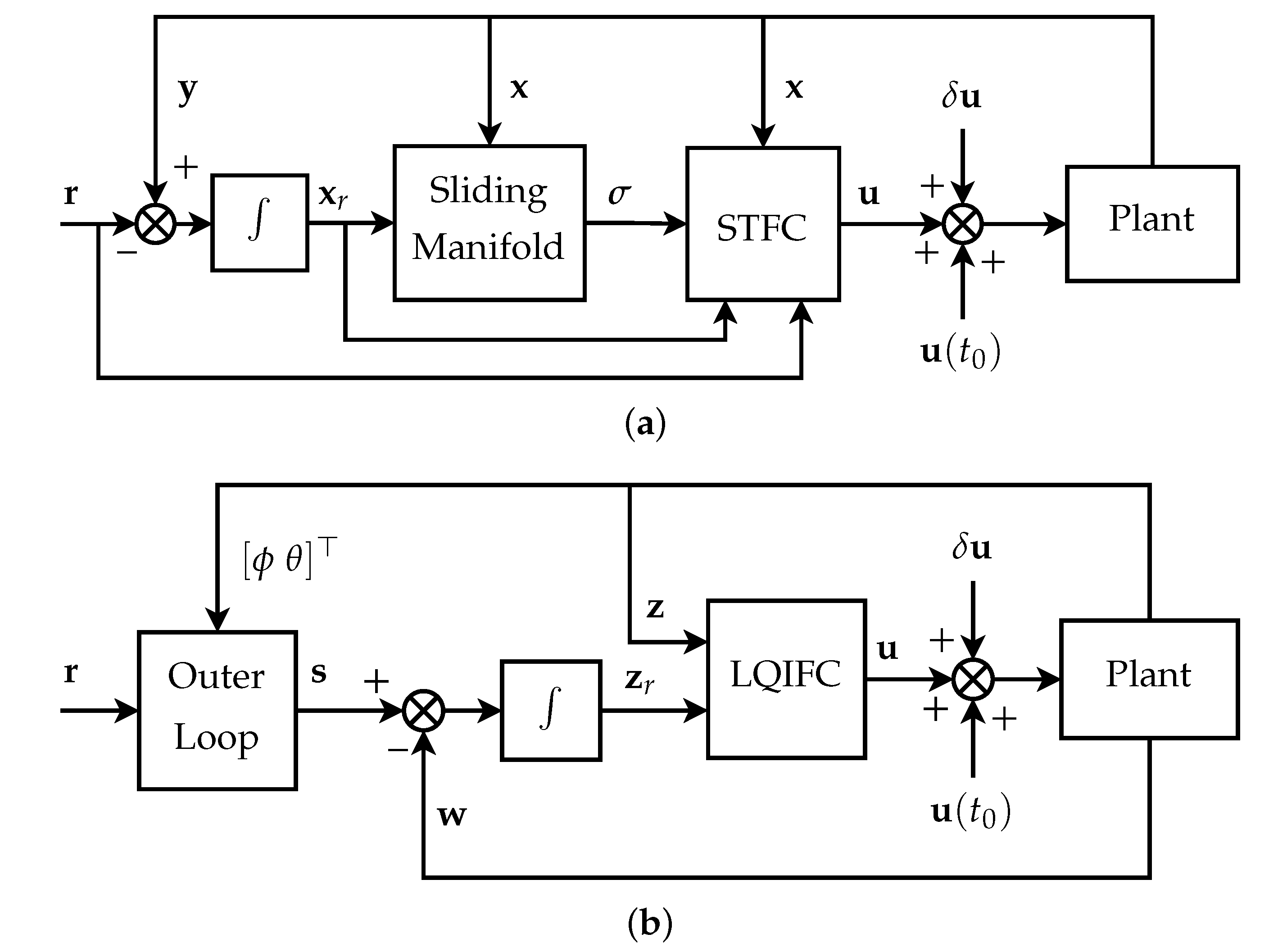
A multivariable, finite-time-convergent, super-twisting flight controller (STFC) based on [23] is synthesized for a helicopter attitude and rate command system. Its multivariable structure respects plant cross-coupling and ensures an identical convergence time for all sliding variables. Unlike References [9,20], estimation of neither the sliding variable derivative nor the exogenous disturbance input is needed, thus offering a simpler yet equally robust controller.
2.
The STFC’s efficacy, chattering alleviation, and finite-time convergence are demonstrated on a nonlinear, higher-order helicopter plant model in atmospheric turbulence. To our best knowledge, this constitutes the first SOSM controller validation on a nonlinear helicopter plant, since Reference [20] used a lower-order, linear plant. Performance comparisons are also presented between the STFC and a linear quadratic flight controller, the latter synthesized along the lines of Reference [24].

2. Model Description

The plant is a nonlinear flight mechanics simulation model of the BO-105 helicopter, which is a two-ton, multipurpose, twin-engine helicopter with a hingeless main rotor and a tail rotor. The model computes cumulative forces and moments produced by the individual structural components—main rotor, tail rotor, fuselage, and empennage—using nonlinear aerodynamic coefficients and wind tunnel data. Specifically, the main and tail rotor dynamics are based on the blade element momentum theory with rigid blade assumptions and analytical inflow models to simulate the zeroth and first harmonics of the blade flap, lead-lag, and torsion modes. Further details on the simulation model are given in References [25,26] and omitted here for brevity. Plant linearization about steady-state trim conditions yields a six degree-of-freedom (6DOF), 8th order model for controller synthesis:
x ˙ ( t ) = A x ( t ) + B u ( t ) + f ( u , t ) , y ( t ) = C x ( t ) ,
where x ϕ θ u v w p q r R 8 represents change from trim states of Euler roll and pitch attitudes, longitudinal and lateral speeds, heave rate, roll, pitch, and yaw rates, respectively. u D θ D α D β D δ R 4 represents three main rotor control inputs (collective, lateral cyclic, longitudinal cyclic), and one tail rotor control input. A R 8 × 8 and B R 8 × 4 are the state and control matrices; the pair ( A , B ) is controllable; and B has full column rank. For the purpose of controller synthesis, full state feedback is used. y ϕ θ w r R 4 is a subset of the state vector that must robustly track a command signal r ϕ c θ c w c r c R 4 .
Figure 1 compares the state responses produced by the nonlinear model (shown in solid lines) and the 8th order state space model of Equation (1) (shown in dashed lines) for a −5% lateral cyclic step input. Note that these dynamic responses do not contain any external disturbance. While the 8th order model generally gives a good match for the evolution of the rigid-body states, it fails to capture the transient effects caused by the rotor dynamics, as seen in the roll rate response ( p ) .
Remark 1.
The model (1) is a quasi-steady lower-order representation of the true plant in that it subsumes the steady-state effects of the higher frequency rotor dynamics.
Assumption 1.
The plant’s internal dynamics i.e., the rotor modes are stable.
Figure 2 plots the open-loop eigenvalues of a 12DOF, 20th order model that is linearized in a similar fashion as (1) but with six additional degrees of freedom–three rotor flap and three rotor lead-lag. Except one unstable longitudinal mode (phugoid), all other fuselage modes are stable. Among the higher-frequency rotor modes, the lead-lag modes are lowly damped but stable, while the flap modes are well damped. This also validates Assumption 1. Note that the 6DOF model (1) will be used for control design, since both direct rotor state measurements as well as accurate estimation of the rotor dynamics in the fuselage are a challenge in practice.
The uncertainty f :   R 4 × R + R 8 represents bounded turbulence acting on the input channels (matched uncertainty), i.e., f = B δ u , where δ u δ D θ δ D α δ D β δ D δ R 4 is the plant input disturbance due to turbulence. Turbulence is simulated by an empirical control equivalent turbulence input (CETI) model that uses filters driven by zero mean, unity covariance, band-limited white noise ( W n ) [20,27]:
δ D β W n ( s ) = 5.99 ( s + 3 ) , δ D α W n ( s ) = 6.07 ( s + 3 ) , δ D δ W n ( s ) = 21.5 ( s + 7.28 ) , δ D θ W n ( s ) = 0.974 ( s + 60 ) ( s + 1.89 ) ( s + 15 ) .
The nature of the turbulence inputs are illustrated in Figure 3. The figure shows the percentage of displacements of the main rotor longitudinal cyclic, main rotor lateral cyclic, main rotor collective, and tail rotor collective simulated for 10 s. To simulate turbulence in closed-loop, these CETI filter outputs are superimposed on the controller output before inserting the sum in the plant model. Note that Equation (2) were obtained from EC135 tests and are primarily applicable in hover and low speed flight. However, due to the similarity of the EC135 and BO105 rotor systems, Equation (2) are assumed to be applicable to the BO105 model. This assumption is also validated by previous works applying the EC135 turbulence filters to a BO105 physical model [28].

3. Response Characteristics and Sliding Manifold Design

3.1. Response Requirements for Good Handling Qualities

Experimental studies into emerging VTOL concepts [1,2,7] suggest that the essential vehicle responses that simplify piloting and guidance tasks are: second-order attitude command attitude hold (ACAH) in the fuselage pitch and roll axes, first-order vertical rate command height hold (RCHH) in the fuselage heave axis, and first-order yaw rate command direction hold (RCDH) in the fuselage yaw axis. Here, an attitude (rate) command is to be understood in the sense that an axial step input, either by a pilot or a guidance system, shall produce second (first) order attitude (rate) responses at the plant output only in the concerned axis; off-axial responses shall be suppressed. The response requirements can be expressed as follows:
ACAH : θ ˙ + 2 ζ θ ω θ θ + ω θ 2 0 t ( θ θ c ) d τ = 0
ϕ ˙ + 2 ζ ϕ ω ϕ ϕ + ω ϕ 2 0 t ( ϕ ϕ c ) d τ = 0
RCDH : r + λ r 0 t ( r r c ) d τ = 0
RCHH : w + λ z 0 t ( w w c ) d τ = 0
The parameters ζ ( · ) , ω ( · ) in Equations (3)–(6) represent the damping and natural frequencies in the second-order response structures, and λ ( · ) represents the inverse time period in the first-order response structures. These parametric values can be tailored to meet vehicle-specific response crtieria. In the present work, the following values are chosen from previous studies into passenger VTOL [1,2,7], which provide a high-bandwidth attitude and rate control system: ω θ = ω ϕ = 2.34 , ζ θ = 0.9 , ζ ϕ = 0.75 , λ r = 4 , and λ w = 0.95 . Figure 4 shows the time- and frequency-domain responses of the specified ideal response characteristics. Note that for second-order pitch and roll ACAH response-types in Equations (3) and (4), the bandwidth is the frequency at which the phase angle between command signal and output signal is −135°. For the first-order RCDH and RCHH response types in Equations (5) and (6), the bandwidth is defined by the cutoff frequency at −3 dB. The bandwidth values shown in the Bode plot in Figure 4b for all four response-types are well above the respective bandwidths required for level 1 handling qualities in Reference [4].

3.2. Sliding Manifold

The response requirement implies that the system states must converge and obey the closed-loop behavior specified in Equations (3)–(6). This requirement motivates the choice of the sliding variable, since by definition the sliding variable shall represent a stable manifold in the system’s state space [17,20]:
σ ( t ) = ϕ ˙ ( t ) + 2 ζ ϕ ω ϕ ϕ ( t ) + ω ϕ 2 t 0 t ( ϕ ϕ c ) d t θ ˙ ( t ) + 2 ζ θ ω θ θ ( t ) + ω θ 2 t 0 t ( θ θ c ) d t w ( t ) + λ w t 0 t ( w w c ) d t r ( t ) + λ r t 0 t ( r r c ) d t , for σ ( t 0 ) = σ 0 0 .
Remark 2.
The relative degree of σ with respect to u is one for the 6DOF model (1) through ϕ ˙ , θ ˙ , w , r ; but the relative degree of σ with respect to the true plant is greater than one due to the presence of higher-order rotor dynamics.
In order for the sliding variable in Equation (7) to be written as a linear combination of the system state, the state vector must include the integral states on the right hand side of Equation (7). To do so, the original state vector x from (1) is augmented with four integral states x r ( t ) = t 0 t ( y ( τ ) r ( τ ) ) d τ to obtain an augmented state vector, written as x ˜ x r x . Recall that y ϕ θ w r and r ϕ c θ c w c r c . Next, x ˜ can be further repartitioned as x ˜ x 1 x 2 for x 1 x r ϕ θ u v R 8 , the indirectly actuated states, and x 2 w p q r R 4 , the directly actuated states. The augmented uncertain system written in compact form is:
x ˜ ˙ ( t ) = A ˜ x ˜ ( t ) + B ˜ u ( t ) T ˜ r ( t ) + f ˜ ( t ) .
The matrices A ˜ , B ˜ , T ˜ , and f ˜ ( t ) are given by:
Aerospace 09 00006 i001
where A 11 R 2 × 2 , A 12 R 2 × 6 , A 21 R 6 × 2 , A 22 R 6 × 6 , B 2 R 6 × 4 , C 1 R 4 × 2 , and C 2 R 4 × 6 .
To represent the sliding variable σ in Equation (7) in terms of the augmented state vector x ˜ , the kinematic relationships ϕ ˙ = p + q sin ϕ tan θ + r cos ϕ tan θ and θ ˙ = q cos ϕ r sin ϕ are utilized. The sliding manifold to be enforced can be written as a function of the augmented state vector:
S = { ( x 1 , x 2 ) : S 1 x 1 + S 2 ( x 1 ) x 2 = S ( x ˜ ) x ˜ = 0 } ,
where
S = [ S 1 S 2 ]
= ω ϕ 2 0 0 0 2 ζ ϕ ω ϕ 0 0 0 0 1 sin ϕ tan θ cos ϕ tan θ 0 ω θ 2 0 0 0 2 ζ θ ω θ 0 0 0 0 cos ϕ sin ϕ 0 0 λ w 0 0 0 0 0 1 0 0 0 0 0 0 λ r 0 0 0 0 0 0 0 1 .
Notice that S 2 is a nonlinear function of the states through sinusoidal pitch and roll attitude terms. From Equations (10)–(12), the sliding variable can be written as:
σ = S 1 x 1 + S 2 ( x 1 ) x 2 = S ( x ˜ ) x ˜ .

3.3. Expected Closed-Loop Behavior

For the choice of sliding manifold in Equation (10), the poles of the system upon the sliding manifold, i.e., when σ = 0 is enforced, can be determined using a regular-form-based approach discussed in Reference [13] (p. 66), and applied previously to a similar sliding manifold in Reference [20]. The key difference between [20] and the present sliding manifold (10) is the state-dependency of S 2 . By the same approach, first, the following coordinate transformation is introduced:
z = T r x ˜
where the orthogonal transformation matrix T r is computed by QR decomposition of the matrix B ˜ . Since the pair ( A , B ) is controllable and rank ( B ) = rank ( B ˜ ) = 4 , the original system can be expressed in a regular form by taking the time derivative of Equation (14) and substituting for the system and control matrices. The augmented system dynamics from Equation (8) (disregarding the uncertainty term) in the new coordinates become:
z ˙ 1 = A ¯ 11 z 1 + A ¯ 12 z 2 T ¯ 1 r ,
z ˙ 2 = A ¯ 21 z 1 + A ¯ 22 z 2 + B ¯ 2 u ,
and written in compact form as:
z ˙ = A ¯ z + B ¯ u T ¯ r ,
where the matrices in the original and new coordinates are related by:
A ¯ A ¯ 11 A ¯ 12 A ¯ 12 A ¯ 22 = T r A ˜ T r , B ¯ 0 B ¯ 2 = T r B ˜ , T ¯ T ¯ 1 0 = T r T ˜
Likewise, the sliding variable from Equation (10) can be written in terms of the new coordinates as:
σ = S ¯ z = S ¯ 1 z 1 + S ¯ 2 z 2 ,
where S ¯ S ¯ 1 S ¯ 2 = ST r
To enforce sliding motion, σ = 0 in the new coordinates, which implies:
σ = S ¯ 1 z 1 + S ¯ 2 z 2 = 0 ,
and hence , z 2 = S ¯ 2 1 S ¯ 1 z 1 = M z 1 .
Substituting Equation (22) into Equation (15), the system dynamics upon the sliding surface are defined by the following relation:
z ˙ 1 = ( A ¯ 11 A ¯ 12 M ) z 1 T ¯ 1 r ,
z 2 = M z 1 .
Thus, from Equation (23), the system poles upon the sliding manifold are simply given by the eigenvalues of the closed-loop system matrix A ¯ cl ( A ¯ 11 A ¯ 12 M ) . In other words, suppose that a controller exists which forces the states of the rotorcraft to lie on the sliding manifold σ = 0 . Then, the closed-loop stability of the rotorcraft is governed by the sliding mode poles, which are the eigenvalues of A ¯ cl . The existence of a continuous, nonlinear, multivariable controller that can enforce the required behavior σ = 0 in finite-time will be established in the following section.
Figure 5 plots the eigenvalues of A ¯ cl as a function of the pitch and roll attitude variations in the S ¯ 2 sub-matrix. The closed-loop heave and yaw modes appear as single poles at 0.95 and 4 , respectively. These values are identical to the specified RCDH and RCHH first-order response-types in Section 3.1. The closed-loop pitch and roll modes appear as complex conjugates whose frequency and damping are nearly identical to the second-order ACAH response-types in Section 3.1. Figure 5a indicates that the closed-loop eigenvalues are invariant to pitch attitude variations in the domain θ 30 , 30 through the submatrix S 2 . However, for roll attitude variations in the domain ϕ 40 , 40 , the closed-loop pitch mode changes its characteristics at high roll angles, as seen in Figure 5b. The remaining closed-loop modes are invariant.

4. Multivariable Finite-Time Super-Twisting Flight Controller

In contrast to conventional pseudo-SMC flight controllers in References [14,15,16,17,18], a fixed-time disturbance observer-based first-order terminal SMC flight controller in Reference [9], and an input-decoupled SOSM flight controller and observer in Reference [20], this section synthesizes a multivariable, finite-time-convergent, super-twisting flight controller (STFC) for the helicopter plant that stabilizes both σ and σ ˙ about the origin. Aside from obviating the need to estimate σ ˙ , the multivariable STFC ensures that all sliding variables simultaneously converge to zero in finite time. The latter property is particularly advantageous in multi-input-multi-output coupled systems.
The time derivative of Equation (13) gives:
σ ˙ ( t ) = S x ˜ ˙ ( t ) + S ˙ x ˜ ( t ) .
Using (8) and (25), one obtains:
σ ˙ ( t ) = S A ˜ x ˜ ( t ) + S B ˜ u ( t ) S T ˜ r ( t ) + S f ˜ ( t ) + S ˙ x ˜ ( t ) .
Assumption 2.
The disturbance S f ˜ ( t ) is assumed to satisfy the Lipschitz condition with Lipschitz constant L.
Remark 3.
The turbulence entering the plant f ˜ ( t ) , which has been identified from flight data in Reference [27], uses a band-limited white noise input of constant power spectrum and covariance. Since S containing constants and sinusoidal terms is bounded, S f ˜ ( t ) along with its derivative are both bounded. The time evolution of S f ˜ ( t ) and its derivative will be further discussed in Section 5.
The following multivariable continuous control law is chosen [23]:
u ( t ) = ( S B ˜ ) 1 S A ˜ + S ˙ x ˜ ( t ) S T ˜ r ( t ) + β σ ( t ) σ ( t ) + α t 0 t σ ( τ ) σ ( τ ) d τ .
where ( S B ˜ ) is square and non-singular by design, · denotes the Euclidean norm, and control gains α , β > 0 .
Remark 4.
The controller (27) is independent of the sliding variable time derivative, i.e., σ ˙ is absent in (27). Furthermore, S ˙ can be derived analytically, since the elements of S contain constants and sinusoidal terms in ϕ and θ alone. Thus, no numerical differentiation or derivative estimation is necessary to implement the continuous controller (27).
Theorem 1
([23]). Let Assumptions 1 and 2 hold. Then the controller (27) drives the trajectories of the system (8) to the sliding manifold (10) in finite-time given by:
T r 2 n σ ( t 0 ) β 1 + M m ( 1 2 α / β )
for M = α + L and m = α L , n being the order of the system (which is 12 for the augmented state vector x ˜ ), and provided that the control gains are set as α > L and β > 2 α .
Proof. 
Substituting the controller (27) into the sliding variable dynamics (26) yields the following:
σ ˙ ( t ) = β σ ( t ) σ ( t ) α t 0 t σ ( τ ) σ ( τ ) d τ + S f ˜ ( t ) .
Let the uncertainty term be denoted as η ( t ) = S f ˜ ( t ) . Then (29) becomes:
σ ˙ ( t ) = β σ ( t ) σ ( t ) α t 0 t σ ( τ ) σ ( τ ) d τ + η ( t ) .
Since η ( t ) satisfies the Lipschitz condition by Assumption 2, denote ξ ( t ) = η ˙ ( t ) and rewrite (30) as:
σ ˙ ( t ) = β σ ( t ) σ ( t ) + μ ( t ) ,
μ ˙ ( t ) = α σ ( t ) σ ( t ) + ξ ( t ) .
The system (31)–(32) is identical to the problem statement in Section 5 of [23]. Using Lemma 1 of [23], both σ ( t ) = 0 and μ ( t ) = 0 are achieved in finite time given by (28), provided α > L and β > 2 α . It follows from (31) that the continuous, multivariable STFC (27) drives both σ and σ ˙ to the origin in finite time given by (28). This implies that the system (8) enters the sliding manifold (10) in finite time and remains on it subsequently. □
The convergence time estimate (28) for the nonlinear plant will be ascertained in the numerical simulations that follow.

5. Numerical Simulations

5.1. Simulation Environment and STFC Gain Setting

The nonlinear plant described in Section 2 is hosted in a real-time-capable Matlab/Simulink-based helicopter simulation environment (see Figure 6 and the Supplementary Material). The STFC implementation is shown in Figure 6a. The state vector x is fed back to the STFC, where first the sliding manifold is computed. Then the STFC control vector is computed according to (27). Turbulence inputs δ u from (2) are superimposed upon the controller output and, combined with the initial control input u ( t 0 ) , are fed to the plant. The plant computes the aerodynamic forces and moments for this combination of inputs, and it outputs the resulting fuselage motions. The band-limited white noise inputs in (2) are scaled such that input disturbance is limited to | δ u | 5 in each control channel. Note that u [ 0 , 100 ] % represents the minimum and maximum permissible plant control inputs.
One of the challenges of super-twisting control is the need for a priori knowledge on the bounds of the disturbance gradient. As mentioned in Assumption 2 and Theorem 1, this bound sets the condition on α and β for the STFC to overcome matched disturbance. In the present case, a numerical approach is pursued. Figure 7 plots the disturbance η and its numerical derivative η ˙ simulated using η = S f ˜ = S B ˜ δ u , with δ u from (2). As observed in the η ˙ plot (Figure 7 bottom), the largest value of the disturbance derivative is seen in the roll channel. Instead of applying these disturbance derivative limits, α and β are set according to the standard deviation of the disturbance derivative in each channel. Although this does not strictly satisfy the condition in Theorem 1, the authors found this to be a good compromise between disturbance rejection and chattering alleviation in the present example. Indeed, it has been shown that the amplitude and frequency of the limit cycles in finite-time controllers arising from unmodeled internal dynamics are functions of the sliding mode gains [29]. Thus, α and β in the present case are set according to: α > diag ( stdev ( η ˙ 1 ) , , stdev ( η ˙ 4 ) ) and β > 2 α . Referring to Figure 7, α = diag ( 200 , 450 , 1200 , 400 ) and β = diag ( 30 , 50 , 80 , 50 ) are used in what follows.

5.2. Linear Quadratic Integral Flight Controller

To benchmark STFC’s performance against an established linear technique, a linear quadratic integral flight controller (LQIFC) is synthesized along the lines of [24]. As shown in Figure 6b, the LQIFC is implemented in a two-loop structure to produce equivalent attitude and rate responses as the STFC. An outer-loop generates the necessary angular rates to track the pitch and roll attitudes appearing in the command signal r ( t ) . To do so, the pitch and roll attitude derivatives obtained from the constraint σ ( t ) = 0 with identical parametric values as (7) are used to generate angular rate commands. To this are added the yaw and heave rate commands from r ( t ) to obtain the command signal s ( t ) for the LQIFC. This outer-loop computation takes the following form:
p c , o ( t ) q c , o ( t ) r c , o ( t ) = Ω 1 2 ζ ϕ ω ϕ ϕ ( t ) ω ϕ 2 t 0 t ( ϕ ϕ c ) d t 2 ζ θ ω θ θ ( t ) ω θ 2 t 0 t ( θ θ c ) d t 0 ,
s ( t ) = p c , o ( t ) q c , o ( t ) 0 r c , o ( t ) + 0 0 w c ( t ) r c ( t )
where Ω is the transformation matrix from the angular rate vector to the derivative of the Euler angle vector. Integral states are defined as z r ( t ) = t 0 t ( s ( τ ) w ( τ ) ) d τ , where w p q w r is a subset of the state vector z u v w p q r . Defining an augmented state-feedback vector z ˜ z z r , an optimal gain matrix K is then computed via the Matlab function lqi(). The choice Q = diag ( [ 0.1 0.1 5 0.1 0.5 0.5 2 4 50 8 ] ) and R = diag ( [ 10 1 1 1 ] ) in the LQIFC design is found to yield the closest match of the plant output response to the constraint σ = 0 . Finally, the optimal state-feedback control law applied to the plant in Figure 6b is u = K z ˜ .

5.3. Results

Controller performance is evaluated for the following two tasks: (a) stabilization from an untrimmed (unsteady) state, followed by (b) step input command tracking. Task (a) is initiated in hover with arbitrary, unsteady initial conditions (sinking with nose down and rightward tilt) x ( t 0 ) = { 10 , 5 } , { 0 , 0 , 6 } m / s , { 0 , 0 , 0 } / s where the steady-state condition to maintain stable hover is x = { 3.8 , 4.7 } , { 0 , 0 , 0 } m / s , { 0 , 0 , 0 } / s . Thus, r = { 3.8 , 4.7 } , 0 m / s , 0 / s . The controller must attempt to stabilize the helicopter within 5 s . Thereafter, task (b) requires the controller to track r = [ { 33.8 , 10.3 } , w c m / s , 0 / s ] within 5 s and hold these values for quick translation at constant altitude and heading. Note here that w c = u sin θ v sin ϕ cos θ + V z , c cos θ cos ϕ (using the inertial to body velocity transformation) is used to regulate inertial vertical speed to V z = 0 . The fulfilment of tasks (a)–(b) for the high-bandwidth command system in (7) under time constraints is expected to evoke aggressive maneuvers.
Figure 8a shows the state evolution with both controllers during tasks (a)–(b). The stabilization task (a) by the STFC evokes up to 40 / s peak pitch rate and 70 / s peak roll rate, whereas the peaks with the LQIFC are relatively smaller. Despite the high peak values, the STFC stabilizes both pitch and roll attitudes to their respective trim values, and regulates the angular and heave rates. The LQIFC evokes oscillatory pitch attitude that takes longer to stabilize, although the remaining states evolve as expected. In the subsequent tracking task (b), the STFC quickly and accurately forces the plant to reach the commanded attitudes with minimum overshoot, whereas the LQIFC evokes oscillatory pitch and roll attitudes. In this task, the STFC shows better heave and yaw rate regulation as compared to the LQIFC. The angular rates with the STFC, however, reveal minor chattering effects.
Figure 8b shows the plant control inputs generated by both controllers. Initial control saturation can be observed in pursuit of the stabilization task (a). Thereafter, the full spectrum of control authority is utilized for the remainder of both tasks. In particular, all STFC inputs are continuous in nature with minor chattering observed in the lateral cyclic ( D α ) , longitudinal cyclic ( D β ) , and tail rotor collective ( D δ ) channels.
Finally, Figure 9 shows the extent to which each controller enforces the sliding manifold constraint (10). The STFC in Figure 9a enforces σ = σ ˙ = 0 , simultaneously for all channels per Theorem 1, and sustains sliding motion thereafter. The reaching time can be observed to be about T r , obs = 3.3 s. The theoretical reaching time calculated using the values: n = 12 , σ ( t 0 ) = 80 , α = 1200 , β = 80 , L = 1000 according to (28) is T r , est = 12.2   s > T r , obs . Note that the roll channel has been used to estimate this reaching time. Although much higher, the theoretical convergence time can be a useful metric for design assurance purposes.
On the contrary, the LQIFC in Figure 9b achieves σ ˙ = 0 but the constraint σ = 0 is inadequately fulfilled during task (a). Later in task (b) the yaw channel of σ diverges from zero. Likewise, the LQIFC fails to satisfy σ = 0 especially during the command tracking of task (b).
The interested reader is referred to the accompanying Supplementary Video showing our helicopter simulation environment and the responses of Figure 8 as viewed from the helicopter cockpit.

5.4. Discussion

The presence of unmodeled internal dynamics in the plant in the form of the higher-frequency rotor states implies that chattering is alleviated but unavoidable. Periodic motion in σ (Figure 9a, top) occurs because the STFC, synthesized using a lower-order linear representation (1) of the true plant, is oblivious to the presence of higher frequency rotor dynamics in the plant. Moreover, the disturbance (2) does not vanish as σ 0 . Together with the compromise on the α and β values, σ being identically zero during the sliding phase cannot be achieved in the present case. Nevertheless, Figure 9a (bottom plot) indicates σ < 10 all through the sliding phase.
Although chattering is mild in the present case, it may pose difficulties in some others, since flight control is typically a safety critical function in most aircraft. Further research is necessary to characterize chattering due to rotor dynamics in the present STFC. Recent results [29] may be a good point of departure in this direction.

6. Conclusions

This paper presented a continuous, multivariable, finite-time-convergent, super-twisting flight controller (STFC) for rotorcraft and demonstrated its efficacy on a nonlinear, higher-order plant model. A sliding manifold of relative degree one with respect to the control input was chosen to represent preferred piloting and guidance responses. The STFC was shown to robustly render the system trajectories convergent to the sliding manifold in finite time under the influence of exogenous disturbance. Simulation results showed the ability of the STFC to quickly stabilize a helicopter from unsteady, untrimmed initial conditions and accurately track command signals under the influence of atmospheric turbulence. True reaching time of the sliding manifold was shown to lie well within its theoretical estimate. The STFC was also shown to be superior to a linear quadratic controller in enforcing the sliding manifold constraint. However, minor chattering was observed due to unmodeled internal dynamics in the form of higher-frequency rotor states.

Supplementary Materials

The following supporting information can be downloaded at: https://www.mdpi.com/article/10.3390/aerospace9010006/s1. Video S1: Closed-loop controller simulation and visualization in FlightGear open-source flight-simulator.

Author Contributions

Conceptualization, problem formulation, derivations, simulations, and result generation, O.H.; technical supervision and review, M.H. All authors have read and agreed to the published version of the manuscript.

Funding

This research has received no external funding.

Acknowledgments

The authors gratefully acknowledge the Technical University of Munich (TUM) for supporting the publication of this article through the TUM Open Access Publication Fund.

Conflicts of Interest

The authors declare no conflict of interest.

References

  1. Perfect, P.; Jump, M.; White, M.D. Handling Qualities Requirements for Future Personal Aerial Vehicles. J. Guid. Control Dyn. 2015, 38, 2386–2398. [Google Scholar] [CrossRef] [Green Version]
  2. Perfect, P.; Jump, M.; White, M.D. Methods to Assess the Handling Qualities Requirements for Personal Aerial Vehicles. J. Guid. Control Dyn. 2015, 38, 2161–2172. [Google Scholar] [CrossRef] [Green Version]
  3. Berger, T.; Tischler, M.B.; Horn, J.F. High-Speed Rotorcraft Pitch Axis Response Type Investigation. In Proceedings of the Vertical Flight Society 77th Annual Forum, Online, 11–13 May 2021. [Google Scholar]
  4. Baskett, B.J. Aeronautical Design Standard-Performance Specification-Handling Qualities Requirements for Military Rotorcraft; Technical Report ADS-33E-PRF; US Army Aviation and Missile Command: Redstone Arsenal, AL, USA, 2000. [Google Scholar]
  5. Padfield, G.D. Helicopter Flight Dynamics, 1st ed.; John Wiley & Sons, Ltd.: Hoboken, NJ, USA, 2007; pp. 269–292. [Google Scholar]
  6. Mettler, B. Identification Modeling and Characteristics of Miniature Rotorcraft, 1st ed.; Springer Science & Business Media: Berlin/Heidelberg, Germany, 2003; pp. 13–25. [Google Scholar]
  7. Geluardi, S.; Venrooij, J.; Olivari, M.; Bülthoff, H.H.; Pollini, L. Transforming Civil Helicopters into Personal Aerial Vehicles: Modeling, Control, and Validation. J. Guid. Control Dyn. 2017, 40, 2481–2495. [Google Scholar] [CrossRef]
  8. Mehling, T.; Halbe, O.; Gasparac, T.; Vrdoljak, M.; Hajek, M. Piloted Simulation of Helicopter Shipboard Recovery with Visual and Control Augmentation. In Proceedings of the AIAA Scitech 2021 Forum, Online, 11–15 & 19–21 January 2021. [Google Scholar]
  9. Huang, Y.; Zhu, M.; Zheng, Z.; Feroskhan, M. Fixed-time Autonomous Shipboard Landing Control of a Helicopter with External Disturbances. Aerosp. Sci. Technol. 2019, 84, 18–30. [Google Scholar] [CrossRef]
  10. Alexis, K.; Papachristos, C.; Siegwart, R.; Tzes, A. Robust Model Predictive Flight Control of Unmanned Rotorcrafts. J. Intell. Robot. Syst. 2016, 81, 443–469. [Google Scholar] [CrossRef]
  11. Alvarenga, J.; Vitzilaios, N.I.; Valavanis, K.P.; Rutherford, M.J. Survey of Unmanned Helicopter Model-Based Navigation and Control Techniques. J. Intell. Robot. Syst. 2015, 80, 87–138. [Google Scholar] [CrossRef]
  12. Utkin, V. Sliding Modes in Control and Optimization; Springer: Berlin/Heidelberg, Germany, 1992. [Google Scholar]
  13. Edwards, C.; Spurgeon, S. Sliding Mode Control: Theory and Applications; CRC Press: Boca Raton, FL, USA, 1998. [Google Scholar]
  14. Spurgeon, S.; Edwards, C.; Foster, N.P. Robust Model Reference Control Using a Sliding Mode Controller/Observer Scheme with Application to a Helicopter Problem. In Proceedings of the IEEE International Workshop on Variable Structure Systems, Tokyo, Japan, 5–6 December 1996. [Google Scholar]
  15. McGeoch, D.; McGookin, E.; Houston, S. MIMO Sliding Mode Attitude Command Flight Control System for a Helicopter. In Proceedings of the AIAA Guidance, Navigation, and Control Conference and Exhibit, San Francisco, CA, USA, 15–18 August 2005. [Google Scholar]
  16. Hess, R.A.; Mallory, N.J. Pseudosliding-Mode Flight Control for Autonomous Rotorcraft Operation. J. Aircr. 2014, 51, 676–681. [Google Scholar] [CrossRef]
  17. Halbe, O.; Hajek, M. Robust Helicopter Sliding Mode Control for Enhanced Handling and Trajectory Following. J. Guid. Control Dyn. 2020, 43, 1805–1821. [Google Scholar] [CrossRef]
  18. Halbe, O.; Mehling, T.; Hajek, M.; Vrdoljak, M. Synthesis and Piloted Evaluation of Advanced Rotorcraft Response Types Using Robust Sliding Mode Control. J. Am. Helicopter Soc. 2021, 66, 1–20. [Google Scholar] [CrossRef]
  19. Levant, A. Sliding Order and Sliding Accuracy in Sliding Mode Control. Int. J. Control. 1993, 58, 1247–1263. [Google Scholar] [CrossRef]
  20. Halbe, O.; Oza, H. Robust Continuous Finite-Time Control of a Helicopter in Turbulence. IEEE Control. Syst. Lett. 2021, 5, 37–42. [Google Scholar] [CrossRef]
  21. Levant, A. Robust Exact Differentiation via Sliding Mode Technique. Automatica 1998, 34, 379–384. [Google Scholar] [CrossRef]
  22. Nagesh, I.; Edwards, C. A Multivariable Super-Twisting Sliding Mode Approach. Automatica 2014, 50, 984–988. [Google Scholar] [CrossRef] [Green Version]
  23. Basin, M.; Panathula, C.B.; Shtessel, Y. Multivariable Continuous Fixed-Time Second-Order Sliding Mode Control: Design and Convergence Time Estimation. IET Control Theory Appl. 2016, 11, 1104–1111. [Google Scholar] [CrossRef]
  24. Shin, J.; Nonami, K.; Fujiwara, D.; Hazawa, K. Model-based optimal attitude and positioning control of small-scale unmanned helicopter. Robotica 2005, 23, 51–63. [Google Scholar] [CrossRef]
  25. Braun, D.; Kampa, K.; Schimke, D. Mission Oriented Investigation of Handling Qualities Through Simulation. In Proceedings of the 17th European Rotorcraft Forum, Berlin, Germany, 24–27 September 1991. [Google Scholar]
  26. Dietz, M.; Maucher, C.; Schimke, D. Addressing Today’s Aeromechanic Questions by Industrial Answers. In Proceedings of the American Helicopter Society Specialists’ Conference on Aeromechanics, San Francisco, California, USA 20–22 January 2010. [Google Scholar]
  27. Seher-Weiss, S.; Von Gruenhagen, W. Development of EC 135 Turbulence Models via System Identification. Aerosp. Sci. Technol. 2012, 23, 43–52. [Google Scholar] [CrossRef]
  28. Srinathkumar, S. Rotorcraft Precision Hover Control in Atmospheric Turbulence via Eigenstructure Assignment. J. Am. Helicopter Soc. 2019, 64, 1–12. [Google Scholar] [CrossRef]
  29. Panathula, C.B.; Rosales, A.; Shtessel, Y.; Basin, M. Chattering analysis of uniform fixed-time convergent Sliding Mode Control. J. Frankl. Inst. 2017, 354, 1907–1921. [Google Scholar] [CrossRef]
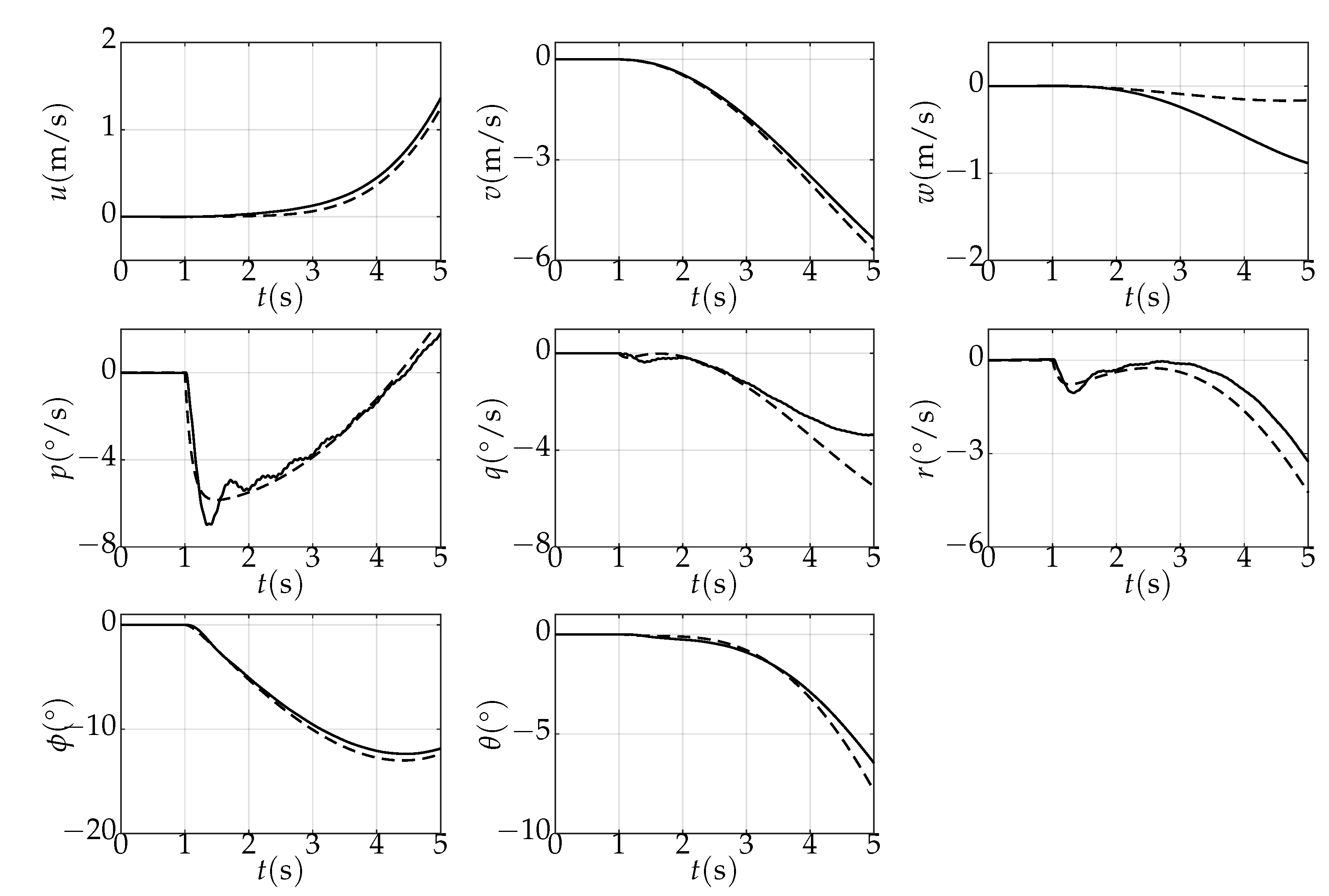
Figure 1. Comparison of state responses to a −5% lateral cyclic step input in hover (—8th order linear state space Equation (1), —nonlinear model).
Aerospace 09 00006 g001
Figure 2. Open-loop eigenvalues showing fuselage and rotor modes in hover.
Aerospace 09 00006 g002
Figure 3. Illustration of control equivalent turbulence inputs applied to the main and tail rotor actuators.
Aerospace 09 00006 g003
Figure 4. Required response characteristics of the attitude command response types. (a) Time response characteristics; (b) Frequency response characteristics.
Aerospace 09 00006 g004
Figure 5. Close-loop eigenvalues (sliding mode poles) of the matrix A ¯ cl ( A ¯ 11 A ¯ 12 M ) in Equation (23) for pitch and roll attitude variations from trim. (a) θ 30 , 30 ; (b) ϕ 40 , 40 .
Aerospace 09 00006 g005
Figure 6. Helicopter simulation environment with two flight controllers. (a) Multivariable finite-time super-twisting flight controller; (b) Linear-quadratic-integral flight controller.
Aerospace 09 00006 g006
Figure 7. Matched disturbance in the sliding dynamics (top) and its derivative (bottom); Aerospace 09 00006 i002w channel, Aerospace 09 00006 i003r channel, Aerospace 09 00006 i004p channel, Aerospace 09 00006 i005q channel.
Aerospace 09 00006 g007
Figure 8. Controller performance during Task (a) stabilization, Plant state responses; Aerospace 09 00006 i006command, Aerospace 09 00006 i007LQIFC, Aerospace 09 00006 i008STFC, and Task (b) command tracking, Controller output applied to plant; Aerospace 09 00006 i009LQIFC, Aerospace 09 00006 i010STFC.
Aerospace 09 00006 g008
Figure 9. Enforcement of specified constraints (sliding manifold) during Task (a) stabilization, STFC; Aerospace 09 00006 i011w channel, Aerospace 09 00006 i012r channel, Aerospace 09 00006 i013 ϕ channel, Aerospace 09 00006 i014 θ channel, Aerospace 09 00006 i015 σ and Task (b) command tracking, LQIFC; Aerospace 09 00006 i016w channel, Aerospace 09 00006 i017r channel, Aerospace 09 00006 i018 ϕ channel, Aerospace 09 00006 i019 θ channel, Aerospace 09 00006 i020 σ .
Aerospace 09 00006 g009
Publisher’s Note: MDPI stays neutral with regard to jurisdictional claims in published maps and institutional affiliations.

