Article

Unmanned Aerial Vehicle Pitch Control under Delay Using Deep Reinforcement Learning with Continuous Action in Wind Tunnel Test

1
Aeronautical Technology Directorate, Japan Aerospace Exploration Agency, Tokyo 181-0015, Japan
2
Department of Aerospace Engineering, University of Bristol, Bristol BS8 1TR, UK
*
Author to whom correspondence should be addressed.
Aerospace 2021, 8(9), 258; https://doi.org/10.3390/aerospace8090258
Submission received: 26 July 2021 / Revised: 9 September 2021 / Accepted: 10 September 2021 / Published: 11 September 2021
(This article belongs to the Special Issue AI/Machine Learning in Aerospace Autonomy)

Abstract

:
Nonlinear flight controllers for fixed-wing unmanned aerial vehicles (UAVs) can potentially be developed using deep reinforcement learning. However, there is often a reality gap between the simulation models used to train these controllers and the real world. This study experimentally investigated the application of deep reinforcement learning to the pitch control of a UAV in wind tunnel tests, with a particular focus of investigating the effect of time delays on flight controller performance. Multiple neural networks were trained in simulation with different assumed time delays and then wind tunnel tested. The neural networks trained with shorter delays tended to be susceptible to delay in the real tests and produce fluctuating behaviour. The neural networks trained with longer delays behaved more conservatively and did not produce oscillations but suffered steady state errors under some conditions due to unmodeled frictional effects. These results highlight the importance of performing physical experiments to validate controller performance and how the training approach used with reinforcement learning needs to be robust to reality gaps between simulation and the real world.

1. Introduction

Machine learning has become a prevalent approach to train controllers for a variety of applications in fields such as robotics, game playing and aviation. Neural networks can be trained to act as nonlinear controllers that can cope with highly nonlinear plant dynamics and accomplish complex tasks. Supervised learning is a common method of training, where neural networks learn from training data generated using baseline controllers. In the aviation domain, supervised learning has been proposed as an alternate decision-making method [1], with the lookup table for a collision avoidance system being replaced with a neural network, to increase the efficiency of the system. Supervised learning has also been applied to flight control systems [2]. For example, the linear gains of an existing control system were replaced with neural networks [3] and the benefits to control performance were validated through simulation. In addition, nonlinear transformations for feedback linearisation have been represented by neural networks with [4] and without [5] recurrent architectures. These examples demonstrate the function approximation abilities of neural networks.
Supervised learning is suited for creating neural networks that can be used as an alternative to an existing flight controller. As part of this process a good baseline controller is required. When an appropriate baseline controller does not exist, or the goal is to improve performance beyond that of an existing controller, supervised learning is not a suitable option. In contrast, deep reinforcement learning is a viable approach to perform training without baseline controllers. Agents with neural-network-based controllers interact with environments and learn to maximise a reward function. The reward function is designed to drive the neural networks to solve a task, e.g., to develop an optimum control law. This process does not require a baseline control system. Through iterative interactions with environments, the controller updates and adapts itself to the task, and learns to be accurate and robust.
The powerful task solving capabilities of deep reinforcement learning were first demonstrated in the game playing area [6,7], and its application has been extended to the field of aviation in recent years. Deep deterministic policy gradient (DDPG) [8] has been applied to trajectory planning, where the neural networks learnt to reach the goal while avoiding specific areas [9]. This simulation study demonstrated successful trajectories and improved efficiency in planner design. DDPG has also been utilised to train controllers for aircraft landing [10]. With the robustness of the controller to wind disturbance being demonstrated through simulation. Unmanned aerial vehicle (UAV) flocking has also been a target for the application of deep reinforcement learning. Using simulation, a flocking controller was trained to control a follower’s roll angle and velocity to keep a certain distance from a leader to avoid collisions [11]. In terms of deep reinforcement learning applied to control the attitude of aircraft, DDPG, trust region policy optimisation (TRPO [12]) and proximal policy optimisation (PPO [13]) algorithms have been used for quadrotors [14]. In these studies control performance was simulated and PPO showed superior accuracy and agility over PID control systems. For fixed-wing UAVs, aerobatic manoeuvres have been controlled based on normalised advantage functions (NAF [15]) [16], and manoeuvres for roll, pitch and airspeed controlled based on PPO [17].
These projects have highlighted the success of the application of deep reinforcement learning to UAV control in a simulation environment; however, using reinforcement learning based controllers in a real environment is known to often be challenging due to gaps between simulation and reality. Recent efforts on closing this gap include experimental work applying a general-purpose flight controller for multirotor UAVs, where translational and rotational accelerations commands are computed and then mapped into rotor speeds, producing a control strategy applicable to various UAV configurations [18]. However, the theoretical performance of trained controllers is often not achieved if the actual aircraft exhibits different dynamics or is subject to external perturbations that are not considered during training. Wind tunnel testing has previously shown the reality gap effect for a UAV’s pitch control using the asynchronous advantage actor-critic (A3C [19]) approach with discrete action spaces [20]. Time delay, which was not included in the training, induced fluctuating pitch behaviour. In contrast to the majority of the previous studies that have only been tested in simulation, this work emphasised the importance of experimental investigation to gauge real world performance.
There have been different possible approaches proposed to reduce the effect of the reality gap between simulation and the real world. In robotics, approaches such as domain randomisation have been used [21]. Training neural networks with some randomised model uncertainties has been shown to help produce controllers which are robust to modelling errors. In such a study, the neural network controllers had a long short term memory (LSTM) layer, which functioned as a time-dependent block and captured the mismatch between simulation and the real world. For UAV flight control, in addition to domain randomisations, an error integral term has been included in the state input, which functioned as the integral term of a PID controller [22] and reduced steady-state drift errors. In this case, the history information was encoded in the integral block. These studies indicate the importance of considering the reality gap in relation to deep reinforcement learning.
This study aimed to gain understanding of the typical relationships between the model error in the training and the consequence of these errors when it comes to real world application. Such knowledge provides the motivation for improving the design of training approaches, and contributes to the understanding of how to develop reliable controllers using reinforcement learning. For this purpose, this study experimentally investigated the attitude control of a fixed-wing UAV using flight controllers developed using a deep reinforcement learning approach. Specifically, the performance of a one-degree-of-freedom pitch controller was examined using wind tunnel tests. The experimental model was inherited from the previous study [20]. This study is different in that the neural network controller has an LSTM layer, which is expected to be an effective measure against time delay, and is trained with a continuous action space in relation to elevator driven manoeuvres, where previously discrete actions were used. Using such a controller, the effect of the time delay was investigated. By varying the time delay in training, various amplitudes of the reality gap for multiple neural network controllers were studied. Through experiments and simulation, the relationship between the training conditions and real world control performance was investigated.

2. Methods

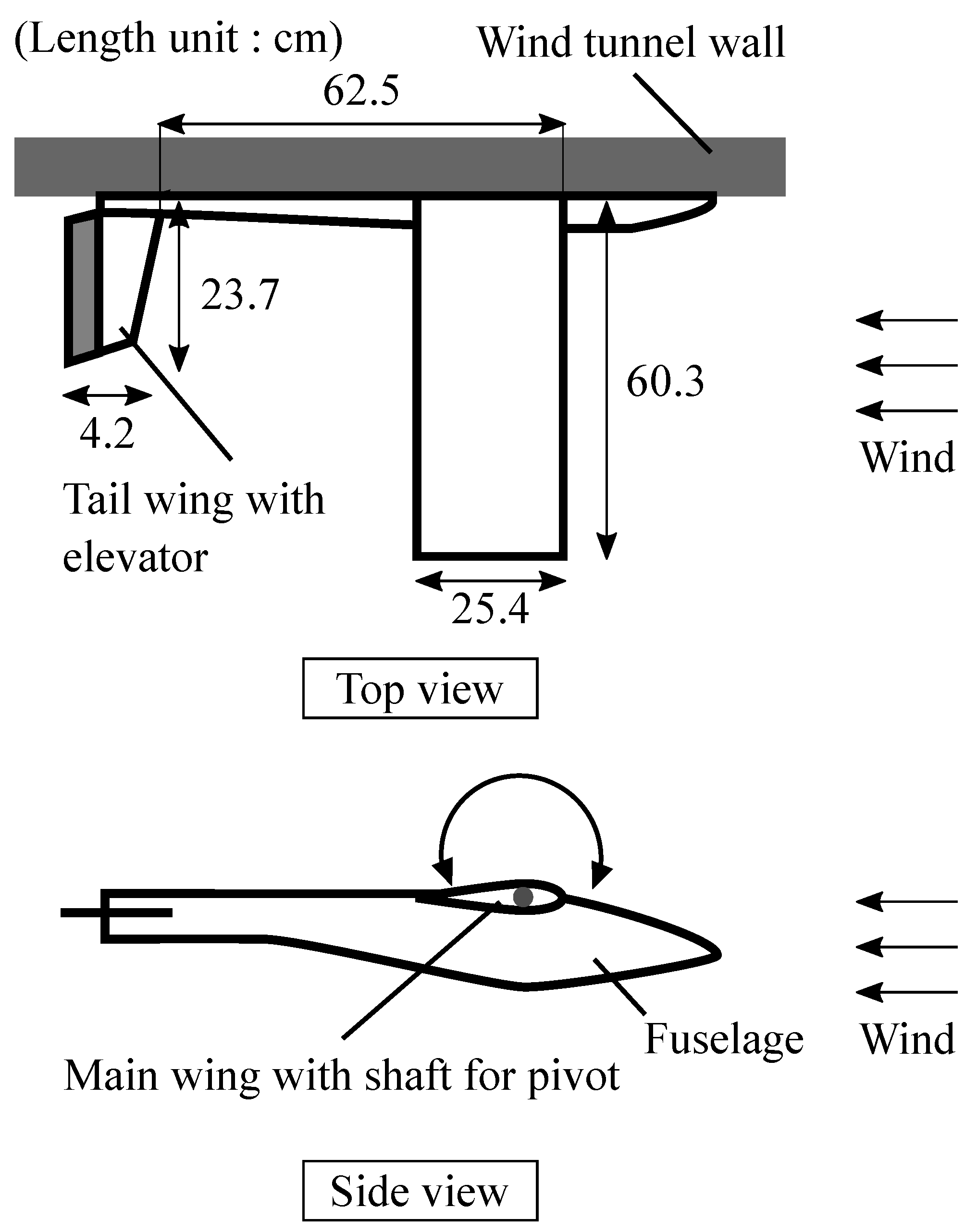
2.1. Experimental Model

The span-wise half of an off-the-shelf radio control aircraft (WOT4 Foam-E Mk2+, Ripmax) was used for the one-degree-of-freedom pitch control experiment as depicted in Figure 1. The model was allowed to pitch freely around the shaft, which was mounted to the side wall of the wind tunnel. The dimensions of the wind tunnel test section were 2.13   m × 1.52   m . The wind speed range in the experiments was 10 m/s to 20 m/s, with the wind speed held constant for each test case. The model was equipped with an air speed sensor (custom-built based on SDP31, Sensirion), a servo motor for the elevator and an inertial measurement unit (IMU)(Pixhawk 1, 3DR) for measuring the pitch angle and pitch rate. These sensors and servo were connected to a microcontroller unit. The microcontroller unit was connected via USB to a computer, which conducted the data recording and signal processing. The signal processing ran at 20 Hz control rate, which was also assumed in numerical simulations. The deep reinforcement learning was completed offline in simulation, and then the trained neural networks were used as an elevator controller for online closed-loop control. The offline training was performed in a Python environment using a custom implementation of the A3C algorithm. In the experiments and numerical simulations, a doublet wave form with an amplitude of 5 ° were given as a target angle-of-attack schedule. The controller performance was evaluated based on the accuracy with which they could follow this schedule.
Two theoretical models were built for the deep reinforcement learning based on results from an elevator sweep experiment, the first one a linear model and the second a linear model incorporating a friction model. To estimate the parameters of the theoretical models, the Output Error Method (OEM) was employed [23]. The OEM was implemented in MATLAB Version 9.6, Release 2019a (MathWorks, Inc., Natick, Massachusetts), using the fmincon algorithm to solve the optimisation problem. A comparison of the response of these models to the experimental data is shown in Figure 2. The angle of attack and pitch rate responses were recorded while the elevator was actuated within ± 45 ° . The wind speed was 14 m/s. The black lines represent the experimental results, with the blue and red lines representing the linear and linear with friction models, respectively. The system cut-off frequency was estimated to be 1.3   Hz . The linear model used to approximate the model dynamics is given by [23]:
I y y α ¨ = 1 2 ρ V 2 S c C M ,
C M = C M 0 + C M α α + C M q c 2 V q + C M δ e δ e ,
where I y y is the moment of inertia for pitch, ρ is the air density, V is the air speed, S is the wing area, c is the chord length, α is the angle of attack, q is the pitch rate and δ e is the elevator angle. Each of the C M x terms represents individual aerodynamic coefficients, and their corresponding identified values are given in Table 1. Note that the identified parameters should capture any wind tunnel wall effects, and that these were considered negligible as the larger part of both lifting surfaces was outside the boundary layer. The simulation results showed larger amplitudes in the angle of attack and pitch rate responses particularly at higher frequencies. In addition, the initiation of the angle of attack variation in response to the elevator sweep at 0 s was instantaneous in simulation, while it showed a delay in the experiment. These differences were related to the effect of friction around the pitching shaft.The linear model incorporating a friction model [24] is given by
I y y α ¨ = 1 2 ρ V 2 S c C M g 4 tanh ( g 5 q ) ,
where only the Coulomb friction effect was considered and the coefficients were estimated as g 4 = 8.53 × 10 1 Nm and g 5 = 100.0 s/rad. The amplitudes of the responses at higher frequencies agreed well with the experiment, and the initiation delay was also in agreement. In this study, the linear model was used for the deep reinforcement learning, which means that the fidelity of the training model was low. The use of this low-fidelity model caused a problem commonly known as a reality gap that emerges when the actual environment is different from the training environment. The high-fidelity friction model was utilised for theoretical analysis of the effect of the reality gap on the control performance.
The system experienced communication time delay between the time at which the controller output was generated in the computer and the time of its arrival at the microcontroller unit connected to the elevator servo. The histogram of the measured delay for 15,000 data points is shown by the red plot in Figure 3. The peak occurred at 15   m s . The blue plot was simulated data by an approximated log-normal probability density function, f ( x ) , expressed as
f ( x ) = 1 ( x t 0 ) σ 2 π exp ( ( log ( x t 0 ) μ ) 2 2 σ 2 ) , for x > t 0 ,
where x is time in milliseconds, t 0 is offset, σ is 1.67 and μ is 5.27 . Note that to match the experimental data t 0 was set as 15   m s . In addition to this type of communication delay, mechanical delays due to physical phenomena such as the elastic deformation of the servo link are expected to have been present. The total effective delay was difficult to measure directly and would have directly affected the control performance. The effect of the time delay on the control performance was investigated by changing t 0 in simulations.

2.2. Training Algorithm

The neural-network-based pitch controllers were trained using A3C, which is a model-free and actor-critic deep reinforcement learning algorithm [19]. Agents have a policy function (actor network) and a value function (critic network). In the training, the policy function is updated in a gradient ascent manner based on the advantage, and the value function is updated in a supervised manner to estimate the advantage. The advantage is the indicator of the merit of performing the selected action. The advantage is calculated by subtracting the action-value from the state-value and helps reducing the variance of the gradient estimation. In this policy-based approach, the policy is applicable to continuous action spaces.
The architecture of the actor (policy) and critic (value) networks is shown in Figure 4. The architecture was empirically designed. The policy and value functions shared the neurons except for the output layer. The first two hidden layers had 128 neurons each with a leaky rectified linear unit (leaky ReLU) activation functions with 0.1 negative slopes. An LSTM layer was used for the third layer. The LSTM layer had recurrent loops that connected previous information to the present action, which functioned as memory modules, i.e., remembering time series of data. This characteristic was expected to be an effective measure against time delay during the control task. In the output layer, the policy output had two neurons that corresponded to deterministic and variation variables, i.e., the mean and the standard deviation of the action probability. The activation functions for the mean and the standard deviation were softsign and softplus, respectively. The value output was linearly activated. The training was conducted in the Pytorch environment. The neural network parameters were initialized by the method described in [25] using a normal distribution. The initialization gain was 0.1 for the hidden layers and 1.0 for the output layer. The input consisted of the five neurons that corresponded to the state elements. They were the error between the target and observed angles of attack, e α = α t a r g e t α , observed angle of attack α , pitch rate q, elevator angle δ e , and wind speed V. The output action was the elevator angle rate. The elevator angle rate rather than the absolute elevator angle was used so that the output was directly used in a penalty function as described later. The range of the elevator angle rate was within ± 300 ° / s . The absolute elevator angle was saturated within the working range of ± 45 ° .
In the training simulations, episodes were set with 30   s duration and 600 time steps, assuming a control rate of 20   Hz . The target angle-of-attack schedules and constant wind speeds were randomly assigned for each episode. The wind speed range was from 8 to 22   m / s . The black lines in Figure 5 show three examples of the target angle-of-attack schedules with different random seeds. The schedules were generated by utilizing the Ornstein–Uhlenbeck process [26], which calculated signals that drifted in the same direction for a longer duration rather than oscillating around the mean. The initial point was randomly set within ± 0.5 ° , and 15 discrete points with 2.14 s intervals were calculated by the process with mean μ = 0 , volatility σ = 2 and reverting rate towards the mean θ = 0.1 . The calculated points are indicated with the circle plots in Figure 5. The adjacent points were linearly interpolated. Eventually, the target angle of attacks varied approximately within ± 10 ° . For reference, the blue line in Figure 5 shows the doublet schedule used to evaluate the control performance after training. In practice, the random angle-of-attack schedules for training do not match with the doublet profile, allowing the generalized performance of the controllers to be explored. For the other state elements, the initial angle of attack was set as α = α t a r g e t , which meant e α = 0 . The initial pitch rate q was randomly set within the range of ± 5 ° / s . During training, state observation noise was applied at every time step. The angle-of-attack and wind speed noise signals were sampled from a normal distribution both with means equal to zero as well as 0.03 ° and 0.1   m / s standard deviations, respectively. The pitch rate noise was sampled from a uniform distribution with mean equal to zero and standard deviation of ± 3   ° / s . The elevator angle state was not measured but calculated from the elevator command values, hence noise was not applied.
The neural networks were trained with the basic A3C algorithm and generalized advantage estimation (GAE) [27]. The calculation details are described in a previous study [20]. The hyperparameters that were empirically chosen for this pitch control task are listed in Table 2. Seven agents collected training data and an Adam optimizer updated the neural networks [28]. The agents learnt to control the aircraft pitch to maximize the expected reward. The reward function was defined as
r = ( | e α | + 0.1 | q | + 0.1 | a | ) ,
where a ( ° / s ) is the action output of the neural network. The pitch rate | q | and the action penalty | a | aimed to contribute to smooth and stable pitch manoeuvres.
To investigate the effect of delay during training, five amplitudes of delay were defined, namely, 0 (no delay), 100, 200, 300 and 400 m s delay. Five neural networks with different random seeds were trained for each delay group, hence 25 agents were trained in total. In the training simulations, the controller action was pooled at every time step and activated after the time delay passed. For ease of implementation, the time delay was held constant throughout each simulation steps and across episodes.

3. Results

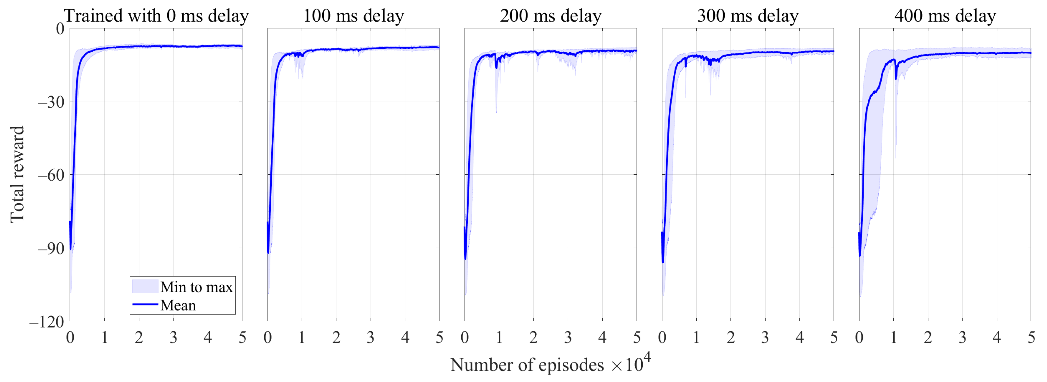
3.1. Training Results

Figure 6 shows the learning curves for the trained neural networks. The groups with larger delays tended to show variations over 5 training samples for the first 2 × 10 4 episodes. However, all the learning curves were saturated to the same total rewards, which indicated successful convergence.
The theoretical control performance of the 25 trained neural networks were investigated in simulation. In simulation, the doublet angle-of-attack target was scheduled, and the stochastic delay expressed in Equation (4) was applied. The delay was calculated and assigned for every time step, and the action output was pooled and activated when the assigned time delay had passed. Only the most recent actions were applied, i.e., when the assigned time delay had passed, the latest action was applied and all other previous actions were discarded. For each neural network, 11 cases of wind speeds from 10 to 20 m / s with a 1 m / s interval were evaluated. For each wind speed 10 simulations were run, each with different random seeds to measure mean performances under random state noise. In total, 110 simulations were run for each neural network. Figure 7 shows the calculated control performance, where the mean total reward over the 110 samples are plotted. Each graph represents one of the five training groups. The neural networks trained with 0   m s delay were labelled as NN0A, NN0B, …, and NN0E. Those with 100   m s delay were NN100A, NN100B, and so on. The letter at the end of each identifier string represents each of the individual neural networks in each training group. To examine delay tolerance, the delay amplitudes were changed by applying t 0 = 15, 50, 100, 150, …, 400 ms, as defined by Equation (4), which corresponded to the horizontal axis in Figure 7. For example, in the 0   m s delay group, the neural networks showed good performance even when the applied delay was t 0 = 15 m s , with a value of approximately −10 for total reward. The performance significantly degraded for larger t 0 values. As seen particularly in the 0, 100 and 200 ms delay groups, severe performance degradation occurred when the applied delay t 0 was larger than the delay assumed for training. This tendency was difficult to infer from individual neural network performance, as some neural networks suffered severe degradation, while others maintained their relative performance. For both the 300   m s and 400   m s delay groups, the performance degradation was limited. Inspection through simulation was critical to gauge the real performance, particularly when the actual delay could be larger than assumed for training. This was because while the delay tolerance differed by individual neural network the learning curves did not show significant differences within the same training group.
Eight neural networks, namely NN0A, NN0B, NN100A, NN100B, NN200A, NN200B, NN300A and NN400A, were chosen and used in both simulations and experiments to produce the results presented in the following sections. They are indicated with blue lines in Figure 7. It was observed that the neural networks trained with larger delay did not always show better performance than the ones trained with smaller delay. For example, NN0B showed higher total reward than NN100A. The same happened for NN100B when compared to NN200A.

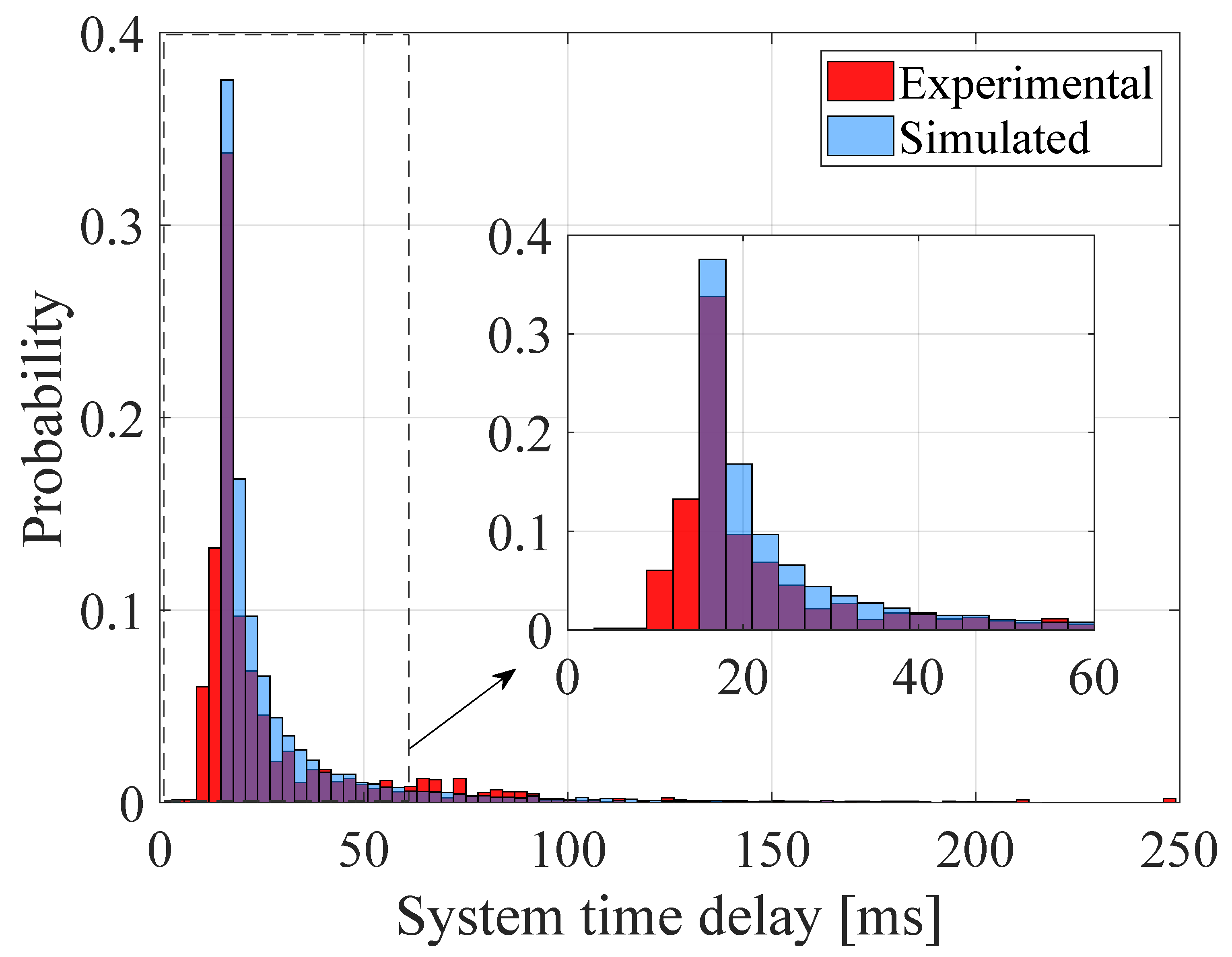
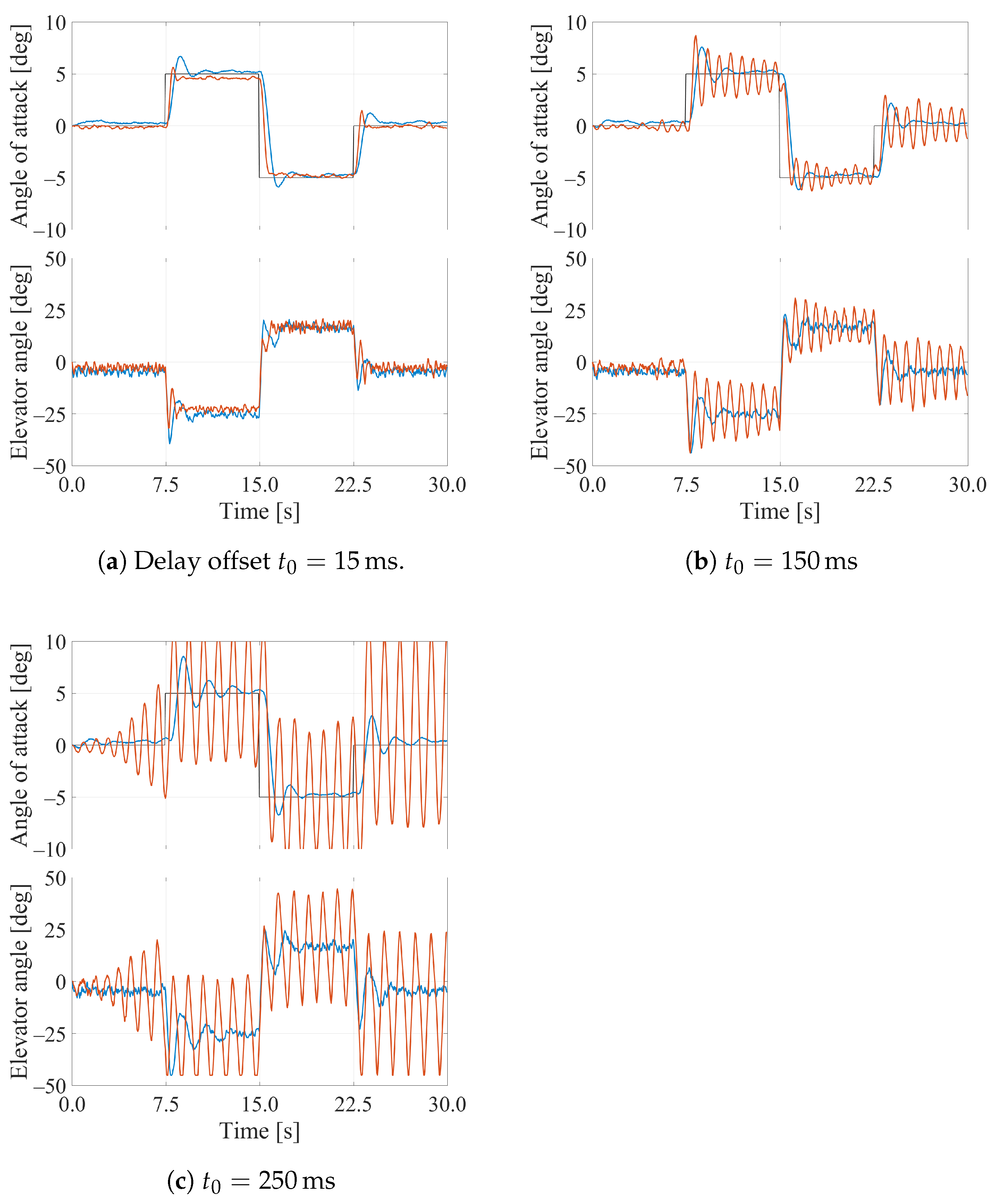
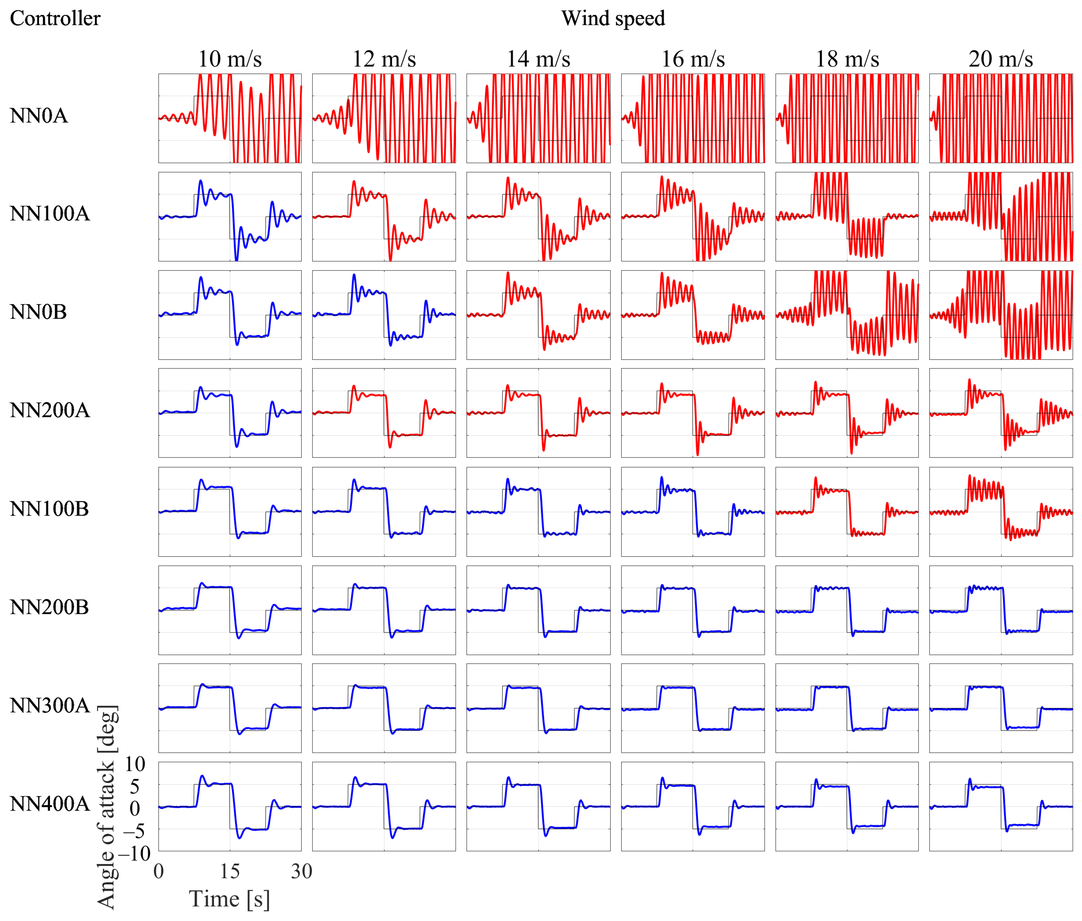
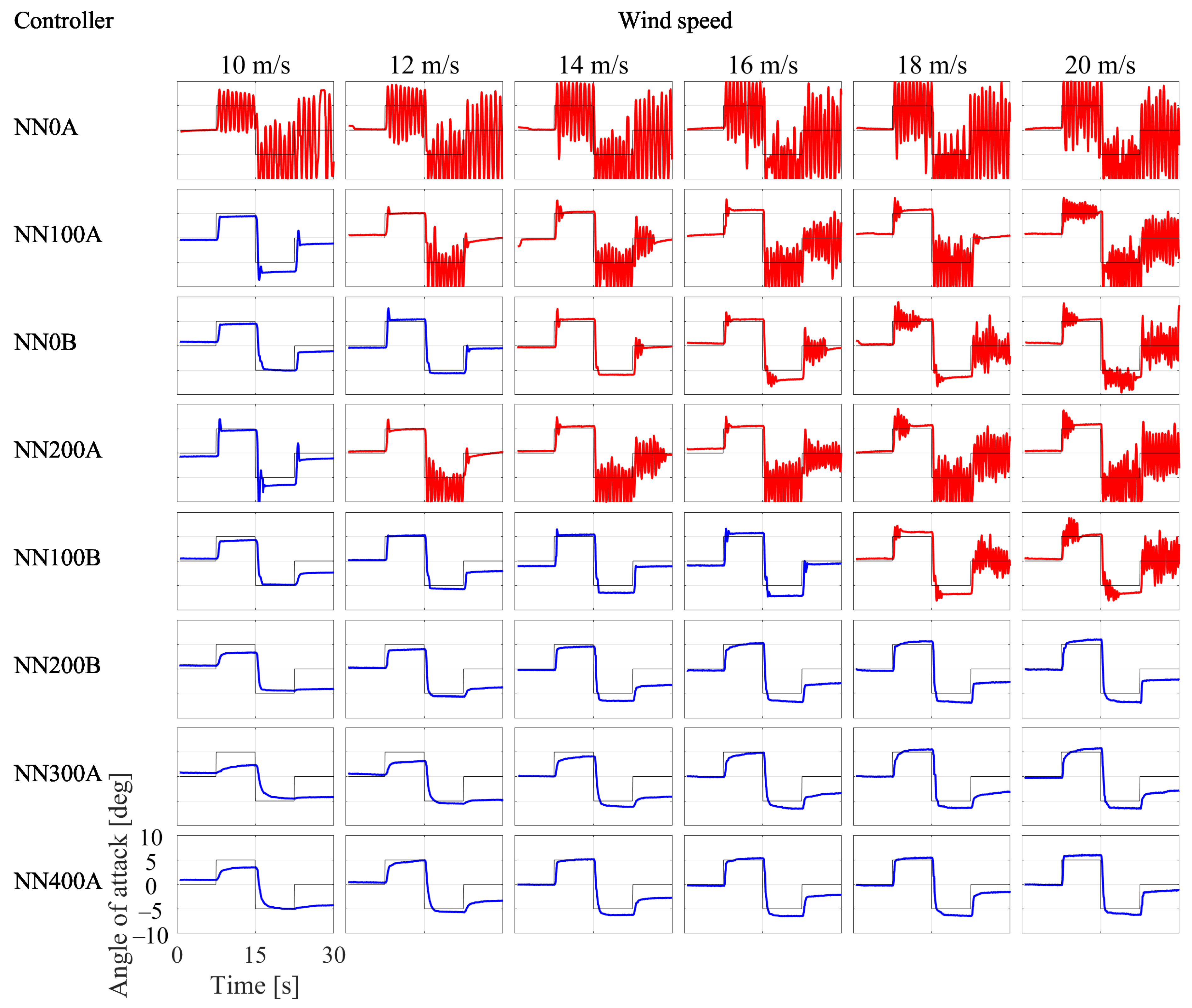
3.2. Simulation Results

To demonstrate examples of theoretical pitch control behaviour, Figure 8 shows simulated angle of attack and elevator manoeuvre histories when NN0B was used as the controller. Delay offsets of t 0 = 15, 150 and 250   m s were applied. Comparing the histories, higher wind speed and larger delays induced fluctuating behaviour, with the corresponding angle of attack fluctuating in response to the elevator manoeuvre. To evaluate and compare these control performances quantitatively, the root mean square error (RMSE) of the angle of attack and the total reward were calculated. For the data collected with NN0B as the controller, both the RMSE and the total reward are shown in Figure 9. In this case, a higher RMSE value and a lower total reward were characteristic of a controller with lower performance. When it comes to the group with t 0 = 150   m s , there was no significant difference in RMSE between the 10 and 20   m / s wind speed cases. However, the RMSE values did not capture the fluctuations observed at 20   m / s wind speed. The RMSE value was sensitive to the offset error at the 0 ° , 5 ° and 5 ° steady phases in the 10   m / s wind speed case, and the effect of the fluctuation at 20   m / s was less evident. On the other hand, the total reward criteria was sensitive to the fluctuations, and agreed with the intuitive quality of control. This was because the pitch rate and action penalties in the reward function effectively weighted the fluctuating behaviour. Empirically, the control simulation results that had a total reward less than −15 were unstable and showed fluctuating behaviour. It was noteworthy that, from a training point of view, reward functions should be sensitive to undesirable behaviour such as fluctuations.

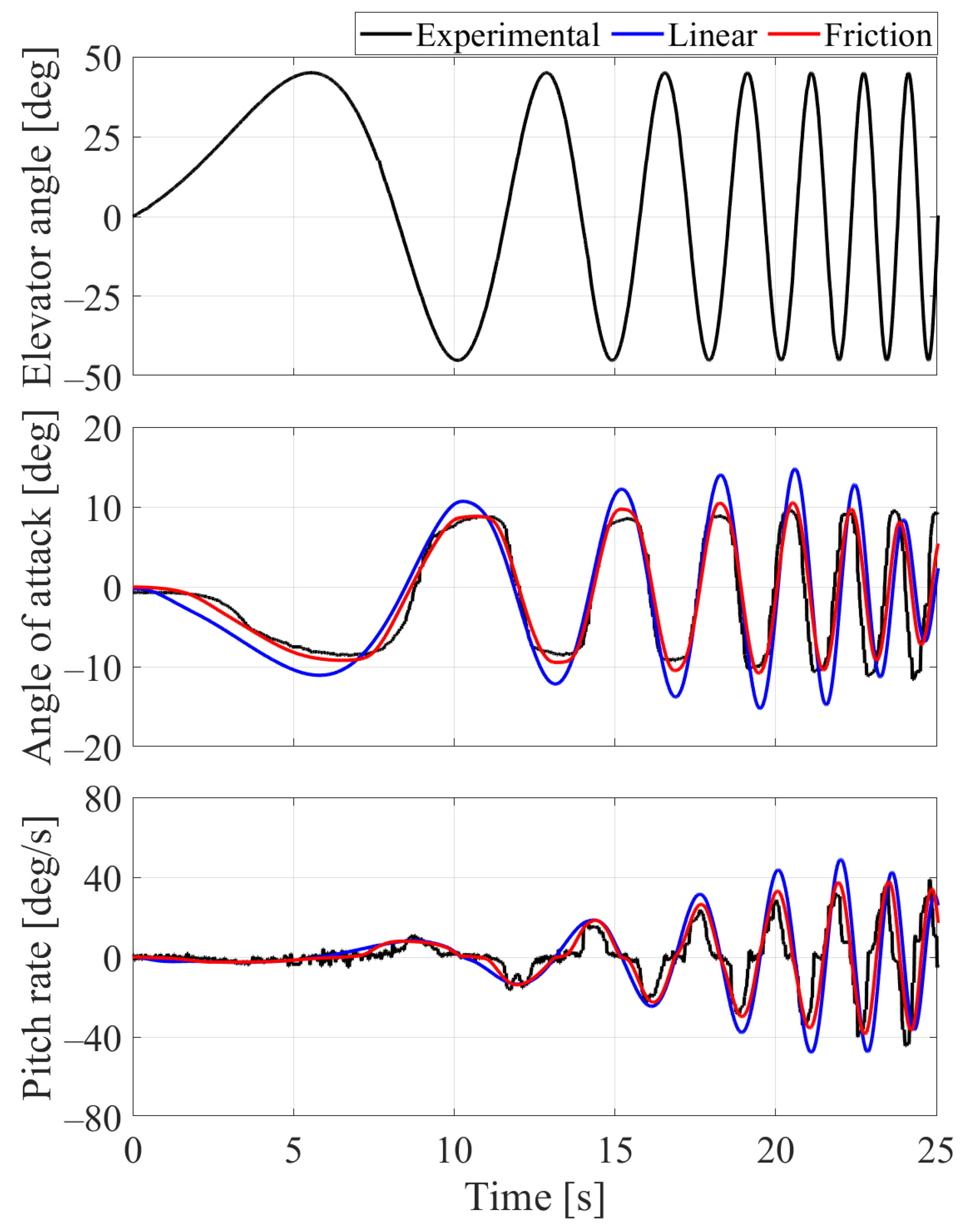
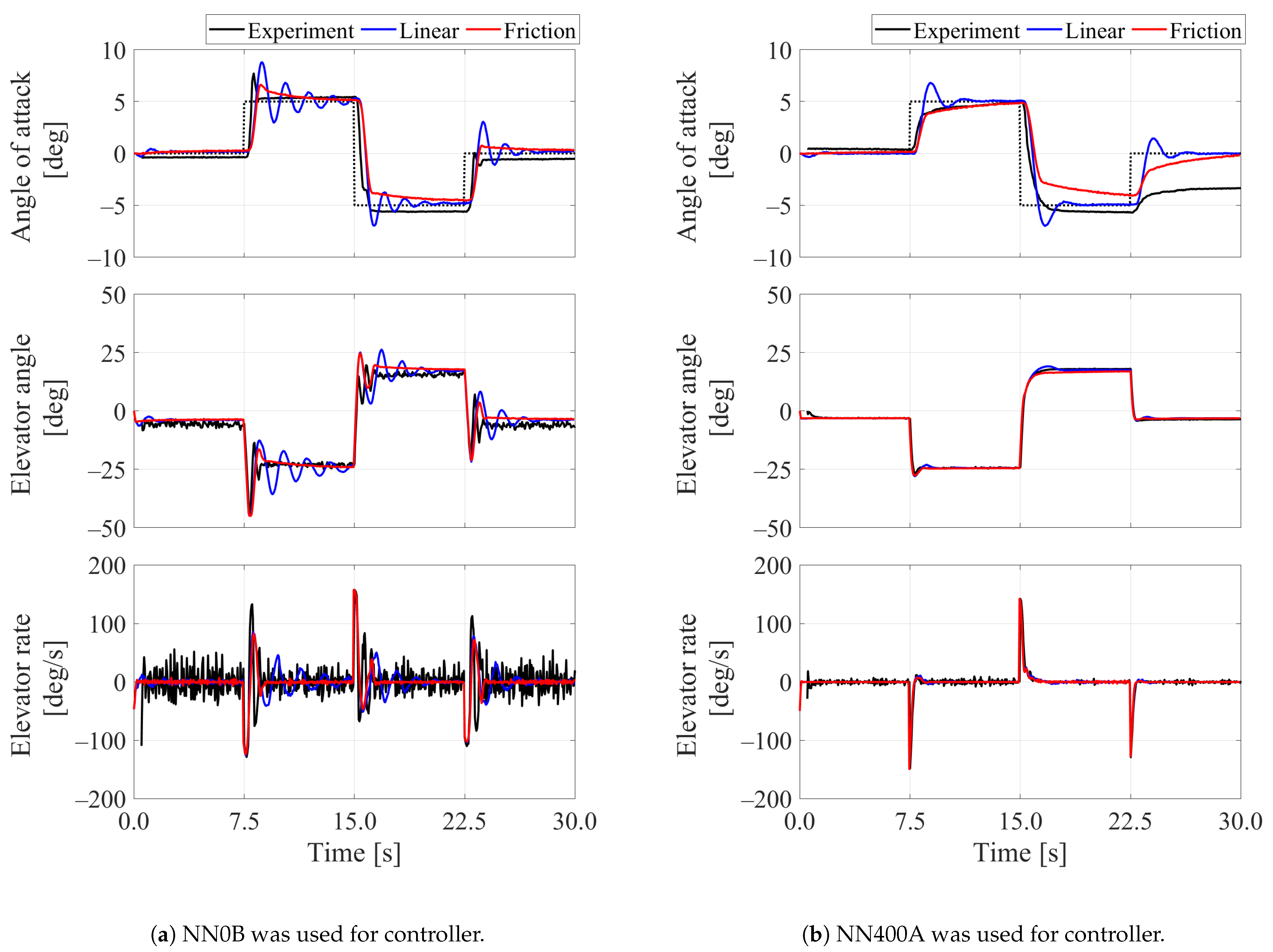
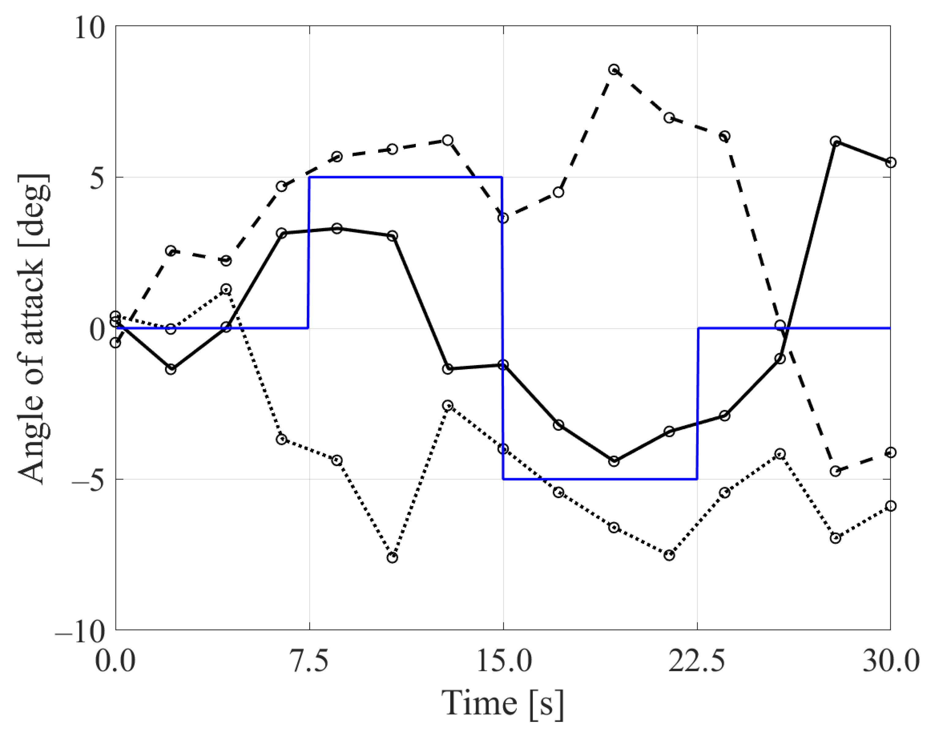
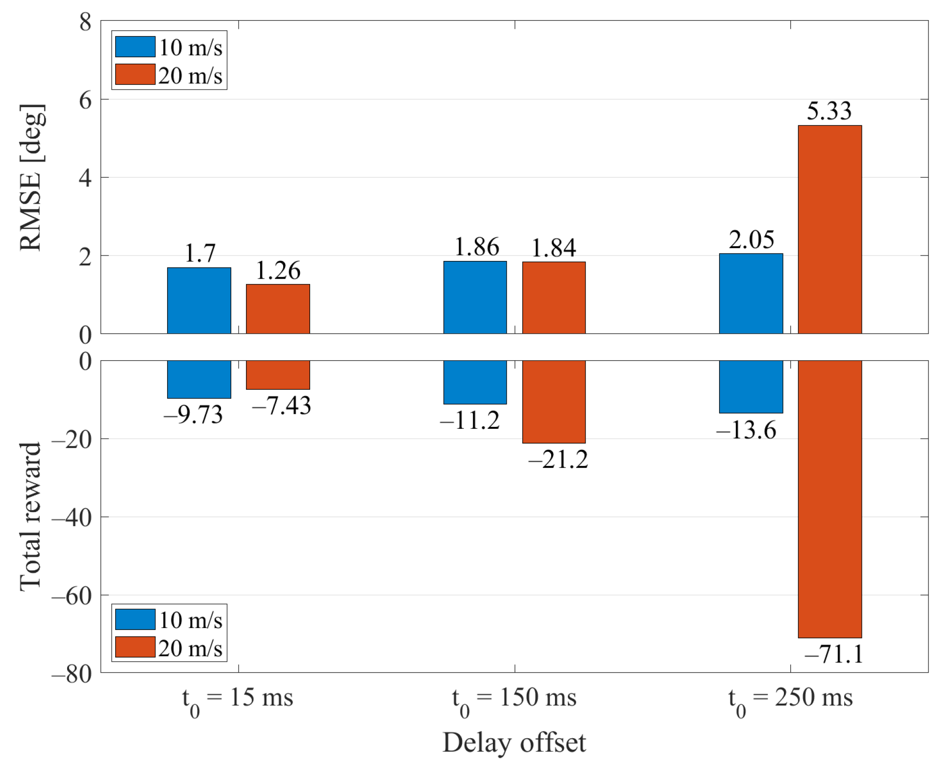
3.3. Experimental Results

Figure 10 shows experimental pitch control results for wind speeds from 10 to 20   m / s . The eight neural network controllers defined in Section 3.1 were used. In Figure 10, the eight neural networks are ordered from top to bottom in the order of the theoretical performance from low to high, as indicated in Figure 7. Under certain wind speed conditions, some controllers experienced fluctuating behaviour, these are plotted in red. These fluctuations were visually judged. The total reward criteria (<−15) could not effectively judge fluctuations because there were steady state errors. The neural networks trained with smaller delay suffered fluctuating behaviour, and higher wind speeds also induced fluctuations. Considering that NN200B and NN300A did not fluctuate, the effective delay, which includes system delay and mechanical delay, was considered to be between 200 and 300   m s . The neural networks trained with larger delay did not suffer fluctuations, however, they tended to exhibit large offset errors. This is particularly evident for lower wind speeds. For example, NN400A with 10   m / s wind speed showed a large offset error for 22.5–30.0 s. This was considered to be due to mechanical friction. There was friction around the pitching shaft and at low wind speeds the model did not produce sufficient moment to rotate to the target α value. When the controllers were trained to be tolerant to delay, they became conservative and tended to avoid rapid manoeuvres. In such cases, the controllers became susceptible to friction effects.
To compare with the theoretical performance, Figure 11 shows simulated pitch control results. In the simulations, a time delay t 0 = 250   m s was applied. The red plot colour scheme was taken from Figure 10, i.e., it indicates the controller and wind speed conditions where fluctuations were observed in the experiment. In general, the fluctuations were satisfactorily reproduced by simulation. It was observed that the simulation study was useful to evaluate theoretical performance and to predict fluctuating behaviour. However, these simulations did not model friction, and hence did not reproduce the offset errors that were observed for cases with lower wind speeds and neural networks trained with larger delays. Therefore, it was essential to conduct experiments to validate the real performance. In addition, comparing the various controllers allowed the estimation of the effective delay. Such an approach, combining parameter study and experimental validation, was effective to identify the reality gap and to select the most suitable controllers.

4. Discussion on Friction Effect

While it was not considered during training, friction existed in the experimental setup. This reality gap was investigated through comparisons between the experiments and simulations that included a friction model. Figure 12 shows pitch control results when NN0B and NN400A are used. The histories of the angle of attack, elevator angle and elevator rate are plotted. The elevator rate corresponded to the neural network output. The experimental results are plotted with black lines. The simulation results using the linear model in Equation (1) are plotted with blue lines and the ones for the friction model in Equation (3) are plotted with red lines. A wind speed of 12   m / s was selected, as both NN0B and NN400A did not exhibit fluctuating control behaviour under this condition. Therefore, the friction effect was noticeable for these controllers. NN0B was trained without delay and therefore resulted in an “aggressive” controller. The elevator rate was unstable in the experiment, and the elevator angle exhibited rapid transitions. The elevator angles in equilibrium were 25 ° and 17 ° for the angle of attacks of 5 ° and 5 ° , respectively, which were overshot in both experiment and simulations. The simulated angle of attack histories showed overshooting behaviour when the linear model was used. For the experiment and simulation with friction results, the angle of attack smoothly transitioned to the target values. On the other hand, NN400A was trained with larger delay and resulted in a “conservative” controller. The elevator rate was stable and the elevator angle smoothly transitioned to the equilibrium angles. These smooth manoeuvres generally produced smaller pitching moments, which contributed to stable control under delay. At the same time, it did not produce sufficient pitching moment when friction was significant. The angle of attack was effectively controlled in the simulation using the linear model, however, large offset errors remained in both the experiment and the simulation with friction.
Considering behaviours of NN0B and NN400A, there was a trade-off. The conservative controller was tolerant to delay but susceptible to friction, while the opposite was true for the aggressive controller. To address these issues, one potential approach is to train controllers with a high-fidelity model that included both delay and friction. This approach is straightforward but not practical in some cases, in particular when obtaining an accurate model is challenging. In this example, the experimental angle of attack for NN400A did not exhibit the offset error for the 5 ° to 5 ° transition, whereas it did for the 5 ° to 0 ° transition. This non-symmetric behaviour would be difficult to predict and model. One of the bottlenecks of the high-fidelity model training approach is that controllers do not accommodate for model error. The elevator angle histories for NN400A were consistent and agreed between the experiment and simulations even though there were clear angle-of-attack errors as seen in Figure 12. This suggests that the controllers simply learnt the equilibrium angles, and they could not adapt to the reality gap. This illustrates one of the limits of the high-fidelity model training approach. To train a controller that is robust to this reality gap, an adaptive approach such as domain randomisation would be another viable option [21]. Model parameters are randomly changed at every episode in training, and as a result, the controllers becomes robust to model uncertainties. This approach will be investigated in future work.
In the majority of previous studies on the application of deep reinforcement learning to UAV attitude control, assessment of control performance has been based on simulation results [16,17]. This study demonstrates the benefit of also considering experimental results. The delay effect was evaluated through experimental and simulated parameter study, and the effective delay threshold was derived. The controllers trained with larger time delays than this effective delay threshold did not exhibit fluctuating behaviour. The comparison between experimental and simulated control behaviour indicated that the friction in the system was non-symmetric and caused offset errors. Based on these results, it is suggested that training approaches that are robust to the reality gap have advantages over simply using higher fidelity models. The experiments not only validated the real control performance but also suggested ways in which training parameters and approaches could be evaluated and designed.

5. Conclusions

An A3C-based deep reinforcement learning was applied to a pitch control task in a wind tunnel test. To investigate tolerance to time delay, five groups of neural networks were trained with different delay assumed in training. The training was successful, and the learning curves had small variations between training samples. However, simulated control performance varied even among the same training groups. Some controllers exhibited severe performance degradation particularly when the applied delay was larger than assumed for training. It was also noted that the stability of the neural networks trained with larger delay was not always better than for the ones trained with smaller delay. This suggest that individual inspections for the trained controllers is essential to understand the real performance.
As a general trend, the neural networks trained with smaller delay were susceptible to delay and suffered fluctuating behaviour. The comparison of fluctuations for the different controllers helped estimating the effective delay in the experimental environment. The effective delay could be used as a threshold, meaning that controllers trained with delay larger than the effective delay could be less likely to exhibit fluctuating behaviour. On the other hand, the neural networks trained with larger delay behaved as conservative controllers and suffered friction effect. This conservative manoeuvring did not produce sufficient pitching moment to rotate the model when friction existed. Nonlinear and non-symmetric dynamics, such as friction, are not always easy to model. This requires a new training approach, where a controller learns to adapt to the difference between training models and actual environments, i.e., when a reality gap exists.
This study’s contribution is to experimentally demonstrate the reality gap effect on an aircraft attitude control task, by considering time delay and friction. They are common concerns for control problems, and also a major challenge for deep reinforcement learning approaches. This study highlights the importance of performing experiments to validate real control performance. The lessons learnt on the effect of the reality gap for a pitch control task can be generalised to different attitude control tasks and different aircraft models. In the future, approaches for mitigating the reality gap will be investigated.

Author Contributions

Conceptualization, D.W., S.A.A.-E. and S.W.; methodology, D.W. and S.A.A.-E.; investigation, D.W. and S.A.A.-E.; data curation, D.W. and S.A.A.-E.; writing—original draft preparation, D.W.; writing—review and editing, D.W., S.A.A.-E. and S.W. All authors have read and agreed to the published version of the manuscript.

Funding

A part of this work was funded by JSPS KAKENHI (grant number JP19K04850). This project has received funding from the European Research Council (ERC) under the European Union’s Horizon 2020 research and innovation programme (grant agreement No 679355).

Acknowledgments

The authors would like to thank Lee Winter from the University of Bristol Wind Tunnel Laboratory, for his invaluable support and work during the assembly of the experimental platform used to carry out the tests presented in this paper.

Conflicts of Interest

The authors declare no conflict of interest.

References

  1. Julian, K.D.; Kochenderfer, M.J. Deep Neural Network Compression for Aircraft Collision Avoidance Systems. J. Guid. Control Dyn. 2019, 42, 598–608. [Google Scholar] [CrossRef]
  2. Gu, W.; Valavanis, K.P.; Rutherford, M.J.; Rizzo, A. A Survey of Artificial Neural Networks with Model-based Control Techniques for Flight Control of Unmanned Aerial Vehicles. In Proceedings of the International Conference on Unmanned Aircraft Systems (ICUAS), Atlanta, GA, USA, 11–14 June 2019; pp. 362–371. [Google Scholar]
  3. Ferrari, S.; Stengel, R.F. Classical/Neural Synthesis of Nonlinear Control Systems. J. Guid. Control Dyn. 2002, 25, 442–448. [Google Scholar] [CrossRef]
  4. Dadian, O.; Bhandari, S.; Raheja, A. A Recurrent Neural Network for Nonlinear Control of a Fixed-Wing UAV. In Proceedings of the American Control Conference (ACC), Boston, MA, USA, 6–8 July 2016; pp. 1341–1346. [Google Scholar]
  5. Kim, B.S.; Calise, A.J.; Kam, M. Nonlinear Flight Control Using Neural Networks and Feedback Linearization. In Proceedings of the First IEEE Regional Conference on Aerospace Control Systems, Westlake Village, CA, USA, 25–27 May1993; pp. 176–181. [Google Scholar]
  6. Mnih, V.; Kavukcuoglu, K.; Silver, D.; Graves, A.; Antonoglou, I.; Wierstra, D.; Riedmiller, M. Playing Atari with Deep Reinforcement Learning. arXiv 2013, arXiv:1312.5602. [Google Scholar]
  7. Mnih, V.; Kavukcuoglu, K.; Silver, D.; Rusu, A.A.; Veness, J.; Bellemare, M.G.; Graves, A.; Riedmiller, M.; Fidjeland, A.K.; Ostrovski, G.; et al. Human-Level Control Through Deep Reinforcement Learning. Nature 2015, 518, 529–533. [Google Scholar] [CrossRef] [PubMed]
  8. Lillicrap, T.P.; Hunt, J.J.; Pritzel, A.; Heess, N.; Erez, T.; Tassa, Y.; Silver, D.; Wierstra, D. Continuous Control with Deep Reinforcement Learning. arXiv 2015, arXiv:1509.02971. [Google Scholar]
  9. Xi, C.; Liu, X. Unmanned Aerial Vehicle Trajectory Planning via Staged Reinforcement Learning. In Proceedings of the 2020 International Conference on Unmanned Aircraft Systems (ICUAS), Athens, Greece, 9–12 June 2020; pp. 246–255. [Google Scholar] [CrossRef]
  10. Tang, C.; Lai, Y.C. Deep Reinforcement Learning Automatic Landing Control of Fixed-Wing Aircraft Using Deep Deterministic Policy Gradient. In Proceedings of the 2020 International Conference on Unmanned Aircraft Systems, ICUAS 2020, Athens, Greece, 9–12 June 2020; pp. 1–9. [Google Scholar] [CrossRef]
  11. Yan, C.; Xiang, X.; Wang, C. Fixed-Wing UAVs flocking in continuous spaces: A deep reinforcement learning approach. Robot. Auton. Syst. 2020, 131, 103594. [Google Scholar] [CrossRef]
  12. Schulman, J.; Levine, S.; Moritz, P.; Jordan, M.I.; Abbeel, P. Trust Region Policy Optimization. arXiv 2015, arXiv:1502.05477. [Google Scholar]
  13. Schulman, J.; Wolski, F.; Dhariwal, P.; Radford, A.; Klimov, O. Proximal Policy Optimization Algorithms. arXiv 2017, arXiv:1707.06347. [Google Scholar]
  14. Koch, W.; Mancuso, R.; West, R.; Bestavros, A. Reinforcement Learning for UAV Attitude Control. arXiv 2018, arXiv:1804.04154. [Google Scholar] [CrossRef] [Green Version]
  15. Gu, S.; Lillicrap, T.; Sutskever, I.; Levine, S. Continuous Deep Q-Learning with Model-based Acceleration. arXiv 2016, arXiv:1603.00748. [Google Scholar]
  16. Clarke, S.G.; Hwang, I. Deep Reinforcement Learning Control for Aerobatic Maneuvering of Agile Fixed-Wing Aircraft. In Proceedings of the AIAA SciTech Forum, Orlando, FL, USA, 6–10 January 2020. [Google Scholar]
  17. Bøhn, E.; Coates, E.M.; Moe, S.; Johansen, T.A. Deep Reinforcement Learning Attitude Control of Fixed-Wing UAVs Using Proximal Policy Optimization. In Proceedings of the 2019 International Conference on Unmanned Aircraft Systems (ICUAS), Cranfield, UK, 25–27 November 2019; pp. 523–533. [Google Scholar]
  18. Pi, C.H.; Dai, Y.W.; Hu, K.C.; Cheng, S. General Purpose Low-Level Reinforcement Learning Control for Multi-Axis Rotor Aerial Vehicles. Sensors 2021, 21, 4560. [Google Scholar] [CrossRef] [PubMed]
  19. Mnih, V.; Badia, A.P.; Mirza, M.; Graves, A.; Lillicrap, T.P.; Harley, T.; Silver, D.; Kavukcuoglu, K. Asynchronous Methods for Deep Reinforcement Learning. arXiv 2016, arXiv:1602.01783. [Google Scholar]
  20. Wada, D.; Araujo-Estrada, S.A.; Windsor, S. Unmanned Aerial Vehicle Pitch Control Using Deep Reinforcement Learning with Discrete Actions in Wind Tunnel Test. Aerospace 2021, 8, 18. [Google Scholar] [CrossRef]
  21. Peng, X.B.; Andrychowicz, M.; Zaremba, W.; Abbeel, P. Sim-to-Real Transfer of Robotic Control with Dynamics Randomization. In Proceedings of the IEEE International Conference on Robotics and Automation, Brisbane, Australia, 21–25 May 2018; pp. 3803–3810. [Google Scholar] [CrossRef] [Green Version]
  22. Xu, J.; Du, T.; Foshey, M.; Li, B.; Zhu, B.; Schulz, A.; Matusik, W. Learning to fly: Computational controller design for hybrid UAVs with reinforcement learning. ACM Trans. Graph. 2019, 38, 1–12. [Google Scholar] [CrossRef]
  23. Jategaonkar, R.V. Flight Vehicle System Identification: A Time Domain Methodology; American Institute of Aeronautics and Astronautics: Reston, VA, USA, 2006. [Google Scholar] [CrossRef]
  24. Makkar, C.; Dixon, W.E.; Sawyer, W.G.; Hu, G. A New Continuously Differentiable Friction Model for Control Systems Design. In Proceedings of the 2005 IEEE/ASME International Conference on Advanced Intelligent Mechatronics, Monterey, CA, USA, 24–28 July 2005; pp. 600–605. [Google Scholar]
  25. Glorot, X.; Bengio, Y. Understanding the difficulty of training deep feedforward neural networks. J. Mach. Learn. Res. 2010, 9, 249–256. [Google Scholar]
  26. Uhlenbeck, G.E.; Ornstein, L.S. On the Theory of the Brownian Motion. Phys. Rev. 1930, 36, 823–841. [Google Scholar] [CrossRef]
  27. Schulman, J.; Moritz, P.; Levine, S.; Jordan, M.I.; Abbeel, P. High-dimensional continuous control using generalized advantage estimation. In Proceedings of the 4th International Conference on Learning Representations, ICLR 2016—Conference Track Proceedings, San Juan, Puerto Rico, 2–4 May 2016; pp. 1–14. [Google Scholar]
  28. Kingma, D.P.; Ba, J. ADAM: A Method for Stochastic Optimization. arXiv 2014, arXiv:1412.6980. [Google Scholar]
Figure 1. Schematic of the aircraft model in the wind tunnel.
Aerospace 08 00258 g001
Figure 2. Elevator command (top) and related angle of attack (middle) and pitch rate (bottom) responses. The wind speed was 14 m/s [20].
Aerospace 08 00258 g002
Figure 3. Histogram of system time delay. The red plots are measured data and the blue plots are simulated data by the approximate equation [20].
Aerospace 08 00258 g003
Figure 4. Neural network architecture.
Aerospace 08 00258 g004
Figure 5. Examples of the angle-of-attack command schedules. Black lines show the schedules used in training with different random seeds. Blue line shows the doublet schedule used to evaluate the control performance.
Aerospace 08 00258 g005
Figure 6. Learning curves. The solid lines are mean learning curves. The shaded areas are the minimum to maximum ranges over 5 random seeds.
Aerospace 08 00258 g006
Figure 7. Simulated mean total reward for the doublet angle-of-attack schedule. Variations of the delay offset t 0 was applied.
Aerospace 08 00258 g007
Figure 8. Simulated angle of attack and elevator angle histories for the NN0B controller. The doublet angle-of-attack schedules were plotted with black lines. Wind speeds were 10 m/s (blue lines) and 20 m/s (orange lines). Applied time delay was t0 = 15 ms (a), 150 ms (b) and 250 ms (c).
Aerospace 08 00258 g008
Figure 9. Root mean square error (RMSE) of the angle of attack (top) and total reward (bottom) for the doublet pitch control when NN0B was used. Wind speeds were 10   m / s (blue) and 20   m / s (orange). The applied time delay was t 0 = 15   m s (left), 150   m s (middle) and 250   m s (right).
Aerospace 08 00258 g009
Figure 10. Experimental pitch control results. Wind speeds were from 10   m / s (left) to 20   m / s (right). The controllers are ordered from top to bottom in the order of theoretical performance in Figure 7. The vertical and horizontal axes correspond to the angle of attack and time, respectively. The target angle-of-attack schedules are shown with black lines. Red plots indicate the results where fluctuating behaviour was observed.
Aerospace 08 00258 g010
Figure 11. Simulated pitch control results. A time delay t 0 = 250   m s was applied. Wind speeds were from 10   m / s (left) to 20   m / s (right). The controllers are ordered from top to bottom in the order of theoretical performance in Figure 7. The vertical and horizontal axes correspond to the angle of attack and time, respectively. The target angle-of-attack schedules are shown with black lines. Red plots indicate the results where fluctuating behaviour was observed in the experiment as seen in Figure 10.
Aerospace 08 00258 g011
Figure 12. Experimental and simulated angle of attack, elevator angle and elevator rate histories. Wind speed was 12 m/s. Applied time delay in simulation was t0 = 250 ms. The doublet angle-of-attack schedules are plotted with black dotted lines. The black, blue and red lines indicate the results of the experiment, simulation with linear model and simulation with friction model, respectively.
Aerospace 08 00258 g012
Table 1. Parameters of wind tunnel model.
ParameterUnitsValue
I y y k g   m 2 1.90 × 10⁻¹
ρ k g / m 3 1.23
S m 2 3.06 × 10⁻¹
c m 2.54 × 10⁻¹
C M 0 −3.00 × 10⁻³
C M α −2.25 × 10⁻¹
C M q −5.46
C M δ e −5.35 × 10⁻²
Table 2. Hyperparameters in deep reinforcement learning.
ParameterValue
Weight for policy loss1
Weight for value loss0.5
Weight for regularization with policy entropy0.01
Discount factor0.99
Number of forward steps in advantage estimation20
Exponential weight parameter in GAE1
Learning rate0.0001
Publisher’s Note: MDPI stays neutral with regard to jurisdictional claims in published maps and institutional affiliations.

