Abstract
To control unmanned aerial systems, we rarely have a perfect system model. Safe and aggressive planning is also challenging for nonlinear and under-actuated systems. Expert pilots, however, demonstrate maneuvers that are deemed at the edge of plane envelope. Inspired by biological systems, in this paper, we introduce a framework that leverages methods in the field of control theory and reinforcement learning to generate feasible, possibly aggressive, trajectories. For the control policies, Dynamic Movement Primitives (DMPs) imitate pilot-induced primitives, and DMPs are combined in parallel to generate trajectories to reach original or different goal points. The stability properties of DMPs and their overall systems are analyzed using contraction theory. For reinforcement learning, Policy Improvement with Path Integrals () was used for the maneuvers. The results in this paper show that updated policies are a feasible and parallel combination of different updated primitives transfer the learning in the contraction regions. Our proposed methodology can be used to imitate, reshape, and improve feasible, possibly aggressive, maneuvers. In addition, we can exploit trajectories generated by optimization methods, such as Model Predictive Control (MPC), and a library of maneuvers can be instantly generated. For application, 3-DOF (degrees of freedom) Helicopter and 2D-UAV (unmanned aerial vehicle) models are utilized to demonstrate the main results.
1. Introduction
Unmanned aerial systems have gained significant importance in the last few decades. Inherently, they are more agile and more suitable for working in dangerous areas in comparison with manned systems. Accordingly, optimization and learning techniques are employed in their applications to increase the number of UAV types and extend their operation range. In [1], centralized path planning based on reinforcement learning is implemented in a combat aerial vehicle fleet in order to avoid enemy defense systems. To localize radio frequency emitting targets in the operation area, multiple UAVs were deployed in [2] using Particle Filter and Extended Kalman Filter algorithms and vision-based detection. For the design optimization and mathematical modeling of unmanned aerial vehicles, a nonlinear lifting line method is proposed in [3]. This new modeling methodology is applied on the Aerospace Research Center (ARC) UAV in order to demonstrate that faster and cheaper prototyping is possible for future UAV models.
Despite enormous advancements in learning and optimization research, generating safe and aggressive movements is a rather hard problem for engineers to solve. Actuator saturation and nonlinear and nonholonomic dynamics are key issues. Most of the applications of UAVs, such as agriculture, intelligence, surveillance, and reconnaissance, only require trimmed flight. However, humans, as well as animals, are experts in generating seemingly hard but stable trajectories despite environmental and dynamic challenges. In acrobatic maneuvers, expert pilots demonstrate maneuvers that are deemed at the edge of the flight envelope.
To generate feasible maneuvers, on the other hand, pilot-executed trajectories are used in [4] to develop nonlinear dynamic models of helicopters. Using this model, intuitive control strategies derived from pilot behaviors are demonstrated in a hardware-in-the-loop simulation environment. Multiple expert executed flight demonstrations are also used in [5] to generate a desired trajectory. Additionally, a receding horizon differential dynamic programming controller is employed for a local model of the helicopter, which is learned from previous flight demonstrations. In [6,7], optimization methods are first employed and then performance is enhanced iteratively through experimentation. In recent years, nonlinear controller designs [8,9,10,11] have also been employed to generate safe maneuvers. For safe path planning [12,13,14,15], on the other hand, cost functions are utilized to minimize the flight envelope. Under these approaches, however, conservative maneuvers are generated in comparison with pilot-induced trajectories.
In general, choosing an optimization/learning methodology is only one aspect of the problem. In many scenarios, it is crucial to guarantee the safety of the system while learning desired behaviors. As a possible solution, Lyapunov-based methods [16,17,18] were proposed to solve reinforcement learning problems. However, there is no common rule for finding a suitable Lyapunov function and using Lyapunov functions; if any such function exists, it does not necessarily result in aggressive maneuvers.
For optimization problems, the stability of the receding horizon scheme can be guaranteed by adding a terminal cost function consisting of a Control Lyapunov Function (CLF) or by applying a sufficient prediction horizon without a terminal cost function, where a general cost function qualifies as Lyapunov function [19]. In [20], Nonlinear Model Predictive Control is applied to a nonholonomic mobile robot with a kinematic model for path following. The stability of the system is guaranteed by appropriately choosing a prediction horizon [21]. As shown in [20], the maneuvers were carefully selected to find the prediction horizon. Similar to reinforcement learning applications, finding a CLF in optimal control problems is not an easy task, and CLF eliminates other possible, may be more effective, solutions. Therefore, such methods lead to conservative solutions in order to guarantee stability.
For biological systems, on the other hand, one can naively guess that learning is achieved by following two sequential steps. First, the movement is imitated, and, next, the imitated behavior is improved through trial and error. It was observed in humans pilots that maneuvers performed with remote helicopters are often repeatable [4]. Each specific maneuver type is predictable in its own sequencing and duration, which suggests a primitive structure. In animals, experiments also show that kittens that have been exposed to adult cats retrieve food much faster in comparison to the control group [22]. Moreover, experiments on monkeys [23,24] also suggest that movements follow a virtual trajectory, which is independent of initial conditions and closely related to feedback control. This finding is also supported by other experiments conducted on frogs [25,26].
The most interesting discovery in the experiments concerning frogs was that the fields generated by activation on the spinal cord follow a principle vectorial summation. Simultaneous stimulation of two different areas of the spinal cord resembles the vectorial summation of the separate activation of each of these areas (See Figure 1) [27]. Generally, it is found that simultaneous stimulation fields and vectorial summations were similar in 87% of the experiments. As mentioned in [28], the vector summation of force fields suggests that nonlinear forms of interactions among neurons and between neurons and muscles is more or less eliminated. With few force fields stored in the spinal cord, one may represent motor primitives using the superposition of spinal fields:
where D and u represent system dynamics and force, respectively. In this equation, force fields () are weighted by scalar and positive coefficients, (). In [28], it is also suggested that these spinal fields are selected using supraspinal signals by evaluating how much each field contributes to the overall field.
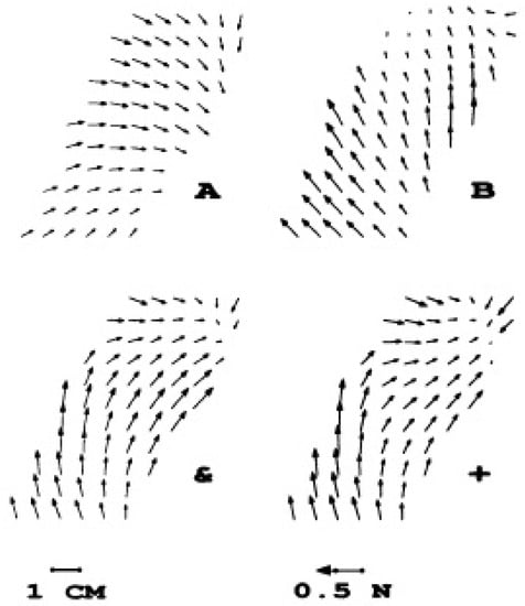
Figure 1.
Costimulation fields (&) and summation fields (+) of (A) and (B) [27].
As a result, this study is focused on learning about and improving feasible trajectories inspired by biological systems. We introduce a framework that leverages methods in the field of control theory and reinforcement learning. We show that we are in the stable flight regime. In practice, inner-loop nonlinear controllers can mainly be used to avoid unmodeled dynamics and disturbances. For primitive structures, DMPs [29] are selected to imitate such primitives of motion. In DMPs, the kinematic trajectories (i.e., positions, velocities, and accelerations) of the motion are generated and converted to motor commands using feedforward controllers, probably by an inverse dynamic model and stabilized by feedback controllers. It is assumed that other non-linearities shall be handled by the controller at the motor execution phase. Detailed definitions of the DMPs can be found in Appendix A. In our study, movement primitives are also combined in parallel to generate feasible trajectories to reach original or different goal points.
Instead of constructing Lyapunov functions for stability, we applied contraction analysis [30] for DMPs, as well as for the reinforcement learning. In general, contraction is a form of stability where all trajectories with different initial conditions contract into a single trajectory. As mentioned in the discussion of previous experiments above, this form of stability is also implied in the structure of virtual trajectories. Additionally, we believe that contraction analysis should be studied for learning, as it was hypothesized in [31] that humans generate stable trajectories so that perturbations have less effect and require little correction; as a result, humans exploit contraction regions.
For reinforcement learning, [32] is used. In , trajectories are updated using stochastic Hamilton–Jacobi–Bellman (HJB) equations and direct policies are learned by approximating a path integral, in which the statistical inference problem is solved using sample roll-outs. Only one open parameter, exploration noise, is required in this learning method, and updates are not limited by numerical instabilities, since neither matrix inversions nor gradient learning rates are needed. As a result, it is shown that the performance of is significantly better than that of gradient-based policy learning, and it can be applied in high-dimensional problems [32].
Although, there are successful studies using pilot-induced trajectories for UAVs, our goal in this research is to design a stable biologically inspired framework, which can be used to imitate and regenerate feasible, possibly aggressive, trajectories. The parallel combination of dynamic movement primitives coupled with reinforcement learning is firstly introduced for motion planning, and contraction analysis is used for the stability analysis. In general, the contribution of this paper is three-fold. First, while DMPs with contraction analysis [33] and with DMPs [32] have been studied before, our proposed methodology in Section 2 encompasses all three methods to generate biologically inspired, feasible and possibly aggressive maneuvers. Second, DMPs are combined in parallel to guarantee stability. Third, it is shown that updated policies are feasible and parallel combination of different updated primitives transfer the learning in contraction regions.
The remainder of the paper is structured as follows. In Section 2, we introduce the methodology and make several remarks for our study. First, DMP can be directly used in controller design, where additional feedback controllers as proposed in [34] are not required. Second, offline learning can be performed using feasible trajectories. Third, having library of motion primitives, one can combine primitives instantly in order to generate feasible trajectories in volatile environments. In Section 3 we demonstrate our results on 3-DOF helicopter and 2D UAV models.
2. Methodology
As mentioned in Section 1, our approach mainly encompasses the methods listed below:
- Contraction Theory.
- Dynamic Movement Primitives.
- Reinforcement Learning Algorithm.
In our methodology, firstly, maneuvers generated by human operators or optimization programs such as MPC are imitated by DMPs. These primitives are then combined in parallel in such a way that the resultant primitive is also contracting. Subsequently, is applied to improve the performance of the combined primitive. For the methodology, we will analyze the compatibility and applicability of these methods and theories below.
2.1. Contraction Analysis of Systems with DMPs
For a system defined below
the system is contracting [30], if the infinitesimal displacement at a fixed time:
decays over time. Therefore, the Jacobian should be a negative definite in that region.
Similar to linearizing the system at equilibrium points, we can use Jacobian to study the convergence of trajectories irrespective of initial conditions. This requirement, however, is a sufficient, but not a necessary, condition. One can define , where is a square matrix, and length is defined , where M is a metric. Hence, the negative definitiveness of a general Jacobian, , is a necessary and sufficient condition for the system to contract [30].
In [33], it is demonstrated that discrete DMPs contract in hierarchy. As DMPs are learned from feasible trajectories, our goal is to study the stability of the system. In other words, we aim to find out if the overall system will contract to the desired trajectories. For the analysis, the system differential equation can be defined in the following form:
Then, virtual displacement dynamics is defined as:
In a scalar case where , the virtual displacement dynamics is reformulated as:
If the reference system is contracting, its effect will be bounded and will decay [30] as , and the system will contract in hierarchy with a proper choice of , so that is uniformly negative. This is analogous to pole placement in linear control theory. Overall, if the system is designed to contract and a particular solution of the system is , the system will converge to the reference trajectory. In general, the stability of these derived feasible trajectories can be studied using several methods in contraction theory, as summarized in Appendix B.
For DMPs, let’s assume the standard manipulator equation [35]:
where is a positive definite inertia matrix, C represents the Coriolis and centripetal forces, g is the force of gravity, q is the joint angle, and u is forces/torques. D also stands for the DMP equations. Since DMP is contracting, its effect on Equation (7) will be bounded, and DMP will act as an exponential decaying disturbance to the original system. As a result, the system contracts to a particular solution with appropriate choices of K.
For the combination of primitives defined in Appendix B, let’s again take the standard manipulator equation with DMPs. If any two or more primitives are contracting, then the linear combination of the reference system in the system dynamics is also contracting such that:
where . It is important to note that, if there is no singularity, any combination of these torques will be within the limits of the torque constraints.
We can combine primitives for the same or different goals as shown in Figure 2. In both approaches, the areas in between primitives are reachable. It is possible to combine primitives that generate trajectories that pass through these areas.
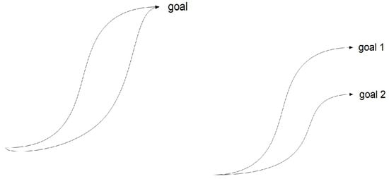
Figure 2.
Primitive Combinations.
One can observe that the combination of system differential equations necessitates the combination of primitives. As a result, only the controlled section of differential equations is modified in Equation (10). Since DMP weights are designed linearly, a simple combination of weights is enough to achieve the desired results. In addition, primitives can also be combined serially. It was shown in [33] that obstacle avoidance maneuvers can be divided into primitives. For this type of combination, it is also possible to modify DMPs using their own parameters.
2.2. Using Reinforcement Learning with Contraction Analysis
In the last few decades, Reinforcement learning has attracted attention as a learning method for studying movement planning and control [36]. Reinforcement learning is a concept that is based on trial and error, typically the constant evaluation of performance in a surrounding environment is also required. In general, reinforcement learning requires an unambiguous representation of states and actions, as well as a scalar reward function.
Reinforcement learning is simple in its form, but it is mostly regarded as impractical due to the curse of dimensionality. Since value function approaches remain problematic in high dimensions, direct policy learning is utilized as an alternative method. Even for direct policy learning, however, numerical issues and the handling of different parameters still need to be addressed.
To compensate for such issues, a new methodology of probabilistic learning was derived on the basis of stochastic optimal control and path integrals. Policy Improvement with Path Integrals () [32] connects between value function approximation using the stochastic HJB equations and direct policy learning by approximating a path integral, that is, by solving a statistical inference problem from sample roll-outs. The resulting algorithm is numerically robust, and only one parameter, exploration noise, is needed for its application.
Such methodology was first applied in stochastic optimal control. For optimal control, the cost functions are defined as:
where is a terminal cost at time , and denotes the immediate cost at time t. Moreover, and R represent the immediate cost at time t and the semi-definite weight matrix of control cost, respectively. For a general system,
we aimed to find a control input, , which minimized the value function:
where is () for all trajectories. The stochastic HJB equation [37,38] for the optimal control problem is shown below:
where .
In [32], optimal control is studied extensively. Subsequently, their study was extended to reinforcement learning, in which a system model is not used. In their approach, the desired state is taken as an input, as action is viewed as any input to the control system. For such a control structure:
Here, Equation (18) generates the desired trajectories. Since only the controlled differential equation is used in path integral formulation, only Equation (18) is needed to apply reinforcement learning. Uncontrolled sections of the system dynamics are not required.
Applying the algorithm to the controlled section of DMPs, the equations of the algorithm [32] are formulated below:
Under this setup, Equation (19) computes the cost function at each time step, i, for each trial, k, in the epoch. Equation (20) represents the projection matrix onto the , i.e., the basis function from the system dynamics, under the metric . Equation (21) determined the probability of each trial. We can simply infer from that lower cost trajectories have higher probabilities. Equation (22) determines the parameter update at each time step. It can easily be seen that trajectories with lower cost contribute more to the parameter update. Equation (23) averages the parameter update, , of each time step. Finally, Equation (24) updates the old parameter.
Using this formulation, we aim to understand the stability aspect of the system, and whether the system contracts from the initial conditions. It was already shown in [33] that discrete DMPs contract. Using hierarchical and other properties of contraction theory, our goal is to find contracting regions for the system setup. One may again find that the probability distribution of serves as a tool for the parallel combination of inputs while updating the desired trajectories. If each roll-out is contracting, we can conclude that the updated trajectories will also be contracting. This is analogous to creating an envelope as shown in Figure 2. We can use controllers, such as the one defined in Equation (44), in order to generate contracting trajectories and apply them to reinforcement learning.
Moreover, each learned DMP is combined in order to generate a new primitive with a different goal point. Such combination is shown below:
where and . Since the new primitive is contracting, we can further continue learning using updates for this primitive. In the learning algorithm (Equation (22)), we see that each parameter, ’s, for K roll-outs is updated as shown below:
Here, probability of the negative cost function is used to weight only the open parameter, i.e., the exploration noise . We assume that the system is contracting with feasible DMPs. Thus, the system always reaches a goal point at the end of the trajectory, and the cost function in can safely beignored. We also assume that q’s will contract to the desired trajectory ’s. Therefore, in a contracting region, we define q’s as a combination of and ’s, which the only parameters to be used in the cost function as shown below:
At each update sequence in a contraction region, the primitive updates are weighted with s. For the combination of primitives (Equation (25)), on the other hand, updates are weighted with s and s, and the probability functions are taken as the average of the probability functions of separate primitives, if we assume that we use the same exploration noise, , for all primitives. Similarly, when we update primitives separately and combine them, we also average the probability functions. As a result, the learning curve of a combined primitive would be improved even further as the primitive learning process continues.
2.3. Remarks
Generally, contraction analysis yields simpler results which can be directly applied to systems/methodologies. In this section, we make a few application remarks, in which contraction analysis is used in combination with DMPs and possible learning methods.
2.3.1. DMP as a Controller
DMPs were originally used in a combination of feedback and feedforward controllers. However, it can be deduced from contraction analysis that one can directly use a DMP in a controller. Consider a system:
where we learn DMPs, and a controller, u, can be generated as . In the closed loop system, particular solution of the system is . Since DMPs are contracting, and the DMP parameters act as PD terms for the overall system, contraction to movement primitives is guaranteed. This controller can be regarded as a system with added virtual springs and dampers, and the path-to-goal point is modified by the basis functions and weights.
2.3.2. Offline Learning
A combination of primitives can be optimized offline without a need for the system model. For example, two primitives for the same goal point can be combined offline, where the weights, , used for the combination are added to 1, such that , where . As shown in Section 2.1, a combined primitive is contracting, given that the original primitives are contracting. Using this setup, one can optimize the combination of the weights in order to improve the performance of the resultant primitive. Subsequently, reinforcement learning can be applied to reshape the primitive again.
2.3.3. Maneuver Library
As defined in Appendix A, DMPs that we used are point attractors. In other words, the system converges to a goal state or equilibrium point. In real life, however, planning requires a change of maneuvers, and we require behaviors where transitions between primitives are needed. Using a controller that guarantees contraction, smooth transitions between primitives can be achieved. Therefore, a library of feasible trajectories must be stored, and we can exploit them in planning. We can create such library by learning feasible trajectories and generate more using the proposed methodology.
3. Application
3.1. The Combination of Primitives for a 3-DOF Helicopter
We used a simplified model derived from a Quanser Helicopter (see Figure 3) in our study. The helicopter is an under-actuated and minimum-phase system with two propellers at the end of its arm. Two DC motors are mounted below the propellers to create the forces which drive propellers. The motors’ axes are parallel and their thrust is vertical to the propellers. There are three degrees of freedom: pitch (the vertical movement of the propellers), roll (the circular movement around the axis of the propellers), and travel (the movement around the vertical base) in contrast with conventional helicopters, which have six degrees of freedom.
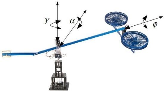
Figure 3.
3-DOF Quanser Helicopter [39].
In the model shown below (see details in [40]), the origin of the coordinate system is at the bearing and slip-ring assembly. The combinations of actuators form the collective () and cyclic () forces, and they are used as inputs in the system. The pitch and roll motions are controlled by collective and cyclic thrust, respectively. The motion in the travel angle is controlled by the components of thrust. A positive roll results in a positive change of angle.
For such a system, feedback linearization (see details in [41]) is used. Control inputs are:
where V is the equivalent input, which can be calculated such that . For the system model described above, aggressive maneuvers mimicking human-operator-generated maneuvers are designed to elevate the pitch angle, , from to and for a possible obstacle-avoidance problem. To reach a goal point between primitives, as shown in in Figure 2, primitives are combined in parallel using proper choices of . Such a maneuver is followed by a 3-DOF Helicopter (see Figure 4). Here, the reference pitch angle reaches .
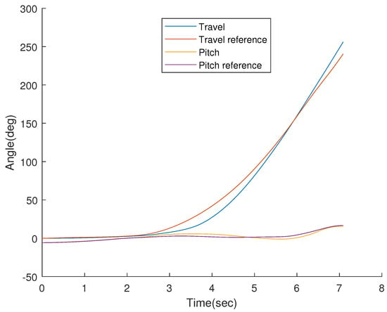
Figure 4.
Tracking of pitch () and travel () angles of a combined primitive.
3.2. MPC Application of Contraction Theory for DMPs
In application, a simple kinematics model will be used to characterize the planar motion of a UAV (see Figure 5). Although there are no dynamics involved, the model is still available to demonstrate nonholonomic motion. Model equations are shown below:
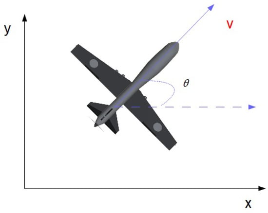
Figure 5.
2D Kinematics Model.
In this 2D model, x and y define the location of the UAV, and is the heading angle. The controller inputs v and w represent the air and angular speed of the UAV, respectively.
The problem can be reformulated as:
The linearized system of the above kinematics cannot be controlled locally since the information of the nonlinear model is lost in system linearization. However, for the nonlinear system, the following result implies that the system is controllable:
where is the Lie bracket of vectors and .
For the model, the desired commands are:
where is the differentiation of = . Using DMPs, the trajectories can be extracted for each state, and controllers can be generated thereafter.
In practice, we will derive feasible trajectories by combining contracting primitives (i.e., DMPs). Our system in Equation (34) can be written with desired inputs:
In this setup, is contracting as is contracting. Additionally, x and y are contracting, since the components of the system equations are contracting. Moreover, DMPs are extracted from feasible trajectories. Hence, we assume that the system is contracting in the close vicinity of the derived trajectories. These primitives can be combined such that:
where and . We can infer from Equations (37) and (38) that any parallel-combined primitive will be within the controller limits of the system. From construction of DMP formulas, we can find that the equilibrium point will be for DMPs.
For such a system, it is also possible to use feedback linearization. For input–output linearization [42], we define an output vector, , and differentiate the output vector two times in order to find input, thus:
where an integrator with a state is added. Defining the system as:
one should note that the resulting controller has a singularity point where .
Through the construction of the DMP formulas, the system will converge to a weighted desired location, , if the desired end points, , are different.
In practice, the flight maneuver defined for starts from the origin, , and ends at specified goal point . Firstly, the MPC application [43] using the CasADi [44] optimization tool is used to generate trajectories (Figure 6).
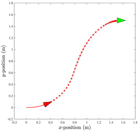
Figure 6.
Flight maneuver where * and ▹ denote prediction horizon and UAV (red: current posture; green: desired posture), respectively.
Then, the DMP is used to imitate each primitive (see Figure 7).
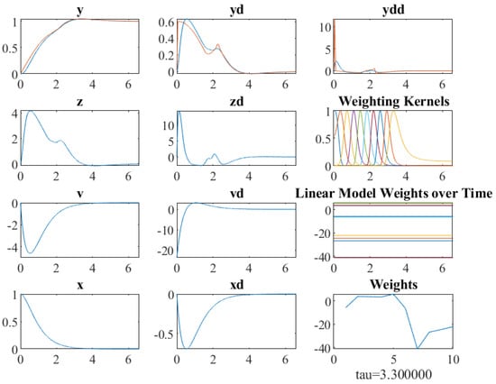
Figure 7.
DMP internals for x-axis.
For parallel combinations, two primitives, as shown in Figure 8, with goal points and are combined using a weighting parameter, , to generate a primitive with a goal point .
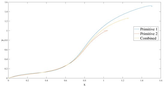
Figure 8.
Combination of DMPs.
Finally, MPC is once again used to follow the combined feasible trajectory (See Figure 9).
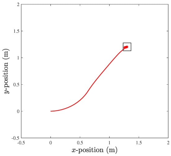
Figure 9.
MPC to follow a new trajectory where □ denotes the UAV.
3.3. The Application of Contraction Theory in Reinforcement Learning ()
For application, the reinforcement learning software [45] is used for a system with a kinematics model defined in Equation (34). For an initial primitive of a flight maneuver with an end point , the DMP imitated the trajectories generated by the MPC algorithm [43]. A total of 100 updates and 10 basis functions/weights was applied. For each update, 10 trials were used. We applied importance sampling in which the five best trials from the previous update were rerun in the next update. The cost function is:
where and are the velocity state vector and weights, respectively. The constants , and are used for penalization. The terminal cost is shown as . The resulting trajectory for x and y is shown in Figure 10.
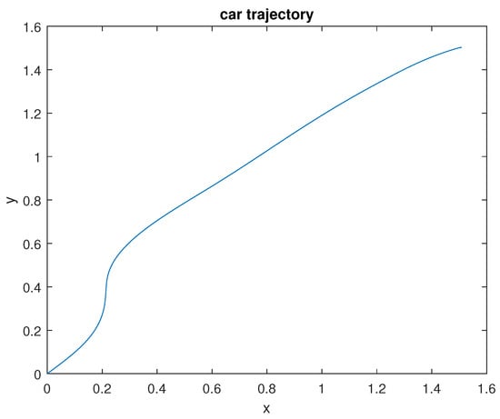
Figure 10.
Flight maneuver where goal point is .
We can also imitate and learn a primitive for a goal point, , using same process. Learning curves for both primitives are shown in Figure 11. After training for both primitives, the primitives were then combined in parallel as defined in Equation (25) in order to generate a stable trajectory, which has a goal point . We observe that learning is transferred in the combined primitive (see Figure 12).
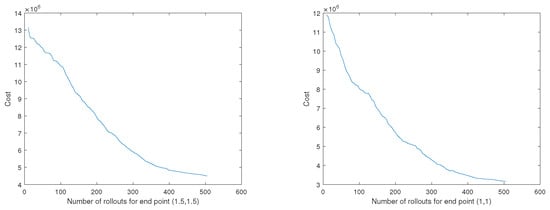
Figure 11.
Learning curves for flight maneuver primitives.
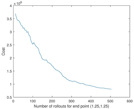
Figure 12.
Learning curve for a combined primitive.
4. Conclusions
Our aim in this paper was to propose a framework that combined several methods to generate maneuvers inspired by biological experiments. In our methodology, stability is addressed with contraction theory, and reinforcement learning is used to improve maneuvers in contraction regions. Our main results are demonstrated on 3-DOF-helicopter and 2D-UAV models. We believe that learning in contraction regions is a key aspect for achieving stable trajectories. Our approach exploits such contracting regions using a combination of primitives. It is shown that trajectories updated by reinforcement learning are feasible, and learning is transferred in contraction regions. It is also possible to employ several other methods, as discussed in our paper, to study the contraction regions around trajectories.
As a part of our future research, we aim to apply this methodology to actual flight platforms. We will focus particularly on scenario-based problems, such as obstacle avoidance, in which serial and parallel combinations of different primitives will be deployed using a maneuver library.
Author Contributions
Conceptualization: B.E.P. and G.I.; methodology: B.E.P. and G.I.; software, B.E.P.; validation: B.E.P. and G.I.; investigation: B.E.P. and G.I.; resources: B.E.P. and G.I.; writing–original draft preparation: B.E.P.; writing–review and editing: B.E.P. and G.I.; visualization: B.E.P. and G.I.; supervision: G.I.; project administration: B.E.P. and G.I. All authors have read and agreed to the published version of the manuscript.
Funding
This research received no external funding.
Institutional Review Board Statement
Not applicable.
Informed Consent Statement
Not applicable.
Data Availability Statement
Not applicable.
Conflicts of Interest
The authors declare no conflict of interest.
Appendix A
In DMPs [34], the goal is to reach an attractor state. A trajectory is generated where transient states of the system are learned by the combination of weights and basis functions. The DMP for a discrete movement can be summarized as follows:
where y, , and represent the desired trajectory; and are time constants; is a temporal scaling factor; and g is the desired goal state. Additionally, a second-order dynamic system can be introduced:
From this setup, it can be shown that system will converge to an attractor point g, when the f-function is assumed to be 0. In DMP, a nonlinear function f is modified in order to learn the desired trajectories between the start and end points.
In Equation (A2), f is a linear combination Gaussian weighting kernels such that:
where:
and , , and represent the bandwidth, the center of the Gaussian kernels, and the weights, respectively.
Appendix B
In general, the stability of the feasible trajectories can be studied using several methods summarized below.
Appendix B.1. Basic Contraction Properties and Matrix Measures
In basic contraction theory, the Jacobian, , should be a uniformly negative definite for system to contract. In other words:
In [46], this result is extended by matrix measures [47]:
where Equation (A7) corresponds to . Matrix measures were used to study the reachability analysis. Furthermore, the Toolbox for Interval Reachability Analysis (TIRA) [48], a MATLAB library that gathers several methods for reachability analysis, is proposed. Following the contraction/growth bound method in TIRA, a state vector is partitioned into components to study reachability.
Appendix B.2. Generalized Contraction Analysis Using Metrics
Appendix B.3. Global Metrics Derived Using Linearization
At equilibrium, one can linearize the system in the form of , and the resulting equation can be defined as . As mentioned in [30], a coordinate transformation, , ( is constant) can be formulated for a Jordan form, thus:
As a result, a generalized Jacobian becomes . This is due to the fact that the system in the equilibrium point, A, should have negative eigenvalues. Therefore, the existence of is guaranteed, and one can apply this metric to find the region of contraction.
Appendix B.4. Combination of Primitives
For the contracting systems defined below:
one can combine their virtual dynamics, as proposed in [30], with positive s such that:
and the combined system will also contract. It is possible to use this methodology to combine primitives. For an identical system, different primitives are defined below:
If the system is combined such that s are positive and , then the particular solutions of each system will contract to the reference trajectory. In other words, the parallel combined system will contract to the linear combination of a reference system, since represents the same system.
References
- Yuksek, B.; Demirezen, U.; Inalhan, G.; Tsourdos, A. Cooperative Planning for an Unmanned Combat Aerial Vehicle Fleet Using Reinforcement Learning. J. Aerosp. Inf. Syst. 2021, 18, 739–750. [Google Scholar] [CrossRef]
- Herekoglu, O.; Hasanzade, M.; Saldiran, E.; Cetin, A.; Ozgur, I.; Kucukoglu, A.; Ustun, M.; Yuksek, B.; Yeniceri, R.; Koyuncu, E.; et al. Flight Testing of a Multiple UAV RF Emission and Vision Based Target Localization Method. In Proceedings of the AIAA Scitech 2019 Forum, San Diego, CA, USA, 7–11 January 2019. [Google Scholar] [CrossRef]
- Karali, H.; İnalhan, G.; Demirezen, M.; Yükselen, M. A new nonlinear lifting line method for aerodynamic analysis and deep learning modeling of small unmanned aerial vehicles. Int. J. Micro Air Veh. 2021, 13. [Google Scholar] [CrossRef]
- Gavrilets, V.; Frazzoli, E.; Mettler, B.; Piedmonte, M.; Feron, E. Aggressive Maneuvering of Small Autonomous Helicopters: A Human Centered Approach. Int. J. Robot. 2001, 20, 795–807. [Google Scholar] [CrossRef]
- Coates, A.; Abbeel, P.; Ng, A. Learning for Control from Multiple Demonstrations. In Proceedings of the 25th International Conference on Machine Learning, Helsinki, Finland, 5–9 July 2008; pp. 144–151. [Google Scholar]
- Lupashin, S.; Schöllig, A.; Sherback, M.; D’Andrea, R. A simple learning strategy for high-speed quadrocopter multi-flips. In Proceedings of the 2010 IEEE International Conference on Robotics and Automation, Anchorage, AL, USA, 3–8 May 2010; pp. 1642–1648. [Google Scholar]
- Levin, J.; Paranjabe, A.; Nahon, M. Agile maneuvering with a small fixed-wing unmanned aerial vehicle. Robot. Auton. Syst. 2019, 116, 148–161. [Google Scholar] [CrossRef]
- Guerrero-Sánchez, M.; Hernández-González, O.; Valencia-Palomo, G.; López-Estrada, F.; Rodríguez-Mata, A.; Garrido, J. Filtered Observer-Based IDA-PBC Control for Trajectory Tracking of a Quadrotor. IEEE Access 2021, 9, 114821–114835. [Google Scholar] [CrossRef]
- Xiao, J. Trajectory planning of quadrotor using sliding mode control with extended state observer. Meas. Control 2020, 53, 1300–1308. [Google Scholar] [CrossRef]
- Almakhles, D. Robust Backstepping Sliding Mode Control for a Quadrotor Trajectory Tracking Application. IEEE Access 2020, 8, 5515–5525. [Google Scholar] [CrossRef]
- Yuksek, B.; Inalhan, G. Reinforcement learning based closed-loop reference model adaptive flight control system design. Int. J. Adapt. Control Signal Process. 2021, 35, 420–440. [Google Scholar] [CrossRef]
- Phung, M.; Ha, Q. Safety-enhanced UAV path planning with spherical vector-based particle swarm optimization. Appl. Soft Comput. 2021, 107, 107376. [Google Scholar] [CrossRef]
- Li, Y.; Liu, C. Efficient and Safe Motion Planning for Quadrotors Based on Unconstrained Quadratic Programming. Robotica 2021, 39, 317–333. [Google Scholar] [CrossRef]
- Lee, K.; Choi, D.; Kim, D. Potential Fields-Aided Motion Planning for Quadcopters in Three-Dimensional Dynamic Environments. In Proceedings of the AIAA Scitech 2021 Forum, Nashville, TN, USA, 11–15 January 2021. [Google Scholar]
- Zhang, X.; Shen, H.; Xie, G.; Lu, H.; Tian, B. Decentralized motion planning for multi quadrotor with obstacle and collision avoidance. Int. J. Intell. Robot. Appl. 2021, 5, 176–185. [Google Scholar] [CrossRef]
- Chow, Y.; Nachum, O.; Duenez-Guzman, E. A Lyapunov-based approachto safe reinforcement learning. In Proceedings of the NIPS 2018, Montréal, QC, Canada, 3–8 December 2018; pp. 8103–8112. [Google Scholar]
- Wenqi, C.; Zhang, B. Lyapunov-regularized reinforcement learning for power system transient stability. arXiv 2021, arXiv:2103.03869. [Google Scholar]
- Perkins, T.; Barto, A. Lyapunov design for safe reinforcement learning. J. Mach. Learn. Res. 2002, 3, 803–832. [Google Scholar]
- Jadbabaie, A.; Hauser, J. On the stability of receding horizon control with a general terminal cost. IEEE Trans. Autom. Control 2005, 50, 674–678. [Google Scholar] [CrossRef] [Green Version]
- Mehrez, M.; Worthmann, K.; Mann, G.; Gosine, R.; Faulwasser, T. Predictive path following of mobile robots without terminal stabilizing constraints. In Proceedings of the 20th IFAC World Congress, Toulouse, France, 11–17 July 2017; pp. 10268–10273. [Google Scholar]
- Grüne, L.; Pannek, J.; Seehafer, M.; Worthmann, K. Analysis of unconstrained nonlinear MPC schemes with varying control horizon. SIAM J. Control Optim. 2010, 48, 4938–4962. [Google Scholar] [CrossRef] [Green Version]
- Galef, B. Imititaion in Animals: History, Definition and Interpretation of Data from the Psychological Laboratory. In Comparative Social Learning; Psychology Press: Hove, UK, 1988; pp. 3–28. [Google Scholar]
- Polit, A.; Bizzi, E. Characteristic of Motor Programs Underlying Arm Movements in Monkeys. J. Neurophsiol. 1979, 42, 183–194. [Google Scholar] [CrossRef]
- Bizzi, E.; Mussa-Ivaldi, F.; Hogan, N. Regulation of multi-joint arm posture and movement. Prog. Brain Res. 1986, 64, 345–351. [Google Scholar]
- Mussa-Ivaldi, F.; Giszter, S.F.; Bizzi, E. Motor Space Coding in the Central Nervous System. Cold Spring Harb. Symp. Quant. Biol. 1990, 55, 827–835. [Google Scholar] [CrossRef]
- Bizzi, E.; Mussa-Ivaldi, F.; Giszter, S. Computations underlying the execution of movement: A biological perpective. Science 1991, 253, 287–291. [Google Scholar] [CrossRef] [Green Version]
- Mussa-Ivaldi, F.A.; Giszter, S.F.; Bizzi, E. Linear combinations of primitives in vertebrate motor control. Proc. Natl. Acad. Sci. USA 1994, 91, 7534–7538. [Google Scholar] [CrossRef] [Green Version]
- Mussa-Ivaldi, F.A.; Bizzi, E. Motor learning through the Combination of Primitives. Philos. Trans. R. Soc. B Biol. Sci. 2000, 355, 1755–1769. [Google Scholar] [CrossRef] [PubMed] [Green Version]
- Schaal, S.; Mohajerian, P.; Ijspeert, A. Dynamics systems vs. optimal control—A unifying view. Prog. Brain Res. 2007, 165, 425–445. [Google Scholar] [PubMed]
- Lohmiller, J.S.W. On Contraction Analysis for Nonlinear Systems. Automatica 1998, 34, 683–686. [Google Scholar] [CrossRef] [Green Version]
- Bazzi, S.; Ebert, J.; Hogan, N.; Sternad, D. Stability and predictability in human control of complex objects. Chaos Interdiscip. J. Nonlinear Sci. 2018, 28, 103103. [Google Scholar] [CrossRef]
- Theodorou, E.; Buchli, J.; Schaal, S. A generalized path integral controlapproach to reinforcement learning. J. Mach. Learn. Res. 2010, 11, 3137–3181. [Google Scholar]
- Perk, B.E.; Slotine, J.J.E. Motion primitives for robotic flight control. arXiv 2006, arXiv:cs/0609140v2. [Google Scholar]
- Ijspeert, A.; Nakanishi, J.; Schaal, S. Learning attractor landscapes for learning motor primitives. In Advances in Neural Information Processing Systems 15; MIT Press: Cambridge, MA, USA, 2003; pp. 1547–1554. [Google Scholar]
- Slotine, J.; Li, W. Applied Nonlinear Control; Prentice-Hall: Hoboken, NJ, USA, 1991. [Google Scholar]
- Suttojn, R.; Barto, A. Reinforcement Learning; MIT Press: Cambridge, MA, USA, 1998. [Google Scholar]
- Stengel, R. Optimal Control and Estimation; Dover Books on Advanced Mathematics; Dover Publications: New York, NY, USA, 1994. [Google Scholar]
- Fleming, W.; Soner, H. Controlled Markov Processes and Viscosity Solutions. In Applications of Mathematics, 2nd ed.; Springer: New York, NY, USA, 2006. [Google Scholar]
- Available online: https://www.quanser.com (accessed on 20 January 2022).
- Ishutkina, M. Design and Implimentation of a Supervisory Safety Controller for a 3DOF Helicopter. Master’s Thesis, Massachusetts Institute of Technology, Cambridge, MA, USA, 2004. [Google Scholar]
- Perk, B.E. Control Primitives for Fast Helicopter Maneuvers. Master’s Thesis, Massachusetts Institute of Technology, Cambridge, MA, USA, 2006. [Google Scholar]
- Luca, A.; Oriola, G.; Vendittelli, M. Control of wheeled mobile robots: An experimental overview. In Ramsete; Nicosia, S., Sicil, B., Bicchi, A., Valigi, P., Eds.; Springer: Berlin, Germany, 2001; Volume 270, pp. 181–226. [Google Scholar]
- Mehrez, M. Github. MPC and MHE Implementation in MATLAB Using Casadi. Available online: https://github.com/MMehrez (accessed on 20 January 2022).
- Andersson, J.; Gillis, J.; Horn, G.; Rawlings, J.; Dieh, M. CasADi: A Software Framework for Nonlinear Optimization and Optimal Control. Math. Program. Comput. 2019, 11, 1–36. [Google Scholar] [CrossRef]
- Theodorou, E.; Buchli, J.; Schaal, S. Path Integral Reinforcement (PI2) Learning Software. Available online: http://www-clmc.usc.edu/Resources/Software (accessed on 20 January 2022).
- Maidens, J.; Arcak, M. Reachability analysis of nonlinear systems using matrix measures. IEEE Trans. Automat. Control 2015, 60, 265–270. [Google Scholar] [CrossRef]
- Desoer, C.; Vidyasagar, M. Feedback Systems: Input-Output Properties; Society for Industrial and Applied Mathematics: Philadelphia, PA, USA, 2009. [Google Scholar]
- Meyer, P.; Davenport, A.; Arcak, M. TIRA: Toolbox for interval reachability analysis. arXiv 2019, arXiv:1902.05204. [Google Scholar]
- Aylward, E.; Parrilo, P.; Slotine, J. Stability and robustness analysis of nonlinear systems via contraction metrics and SOS programming. Automatica 2008, 48, 2163–2170. [Google Scholar] [CrossRef] [Green Version]
- Manchester, I.; Tang, J.; Slotine, J. Unifying robot trajectory tracking with control contraction metrics. In Robotics Research; Springer: Cham, Switzerland, 2018; pp. 403–418. [Google Scholar]
Publisher’s Note: MDPI stays neutral with regard to jurisdictional claims in published maps and institutional affiliations. |
© 2022 by the authors. Licensee MDPI, Basel, Switzerland. This article is an open access article distributed under the terms and conditions of the Creative Commons Attribution (CC BY) license (https://creativecommons.org/licenses/by/4.0/).