Variational Bayesian Iteration-Based Invariant Kalman Filter for Attitude Estimation on Matrix Lie Groups

Abstract

Motivated by the rapid progress of aerospace and robotics engineering, the navigation and control systems on matrix Lie groups have been actively studied in recent years. For rigid targets, the attitude estimation problem is a benchmark one with its states defined as rotation matrices on Lie groups. Based on the invariance properties of symmetry groups, the invariant Kalman filter (IKF) has been developed by researchers for matrix Lie group systems; however, the limitation of the IKF is that its estimation performance is prone to be degraded if the given knowledge of the noise statistics is not accurate. For the symmetry Lie group attitude estimation problem, this paper proposes a new variational Bayesian iteration-based adaptive invariant Kalman filter (VBIKF). In the proposed VBIKF, the a priori error covariance is not propagated by the conventional steps but directly calibrated in an iterative manner based on the posterior sequences. The main advantage of the VBIKF is that the statistics parameter of the system process noise is no longer required and so the IKF’s hard dependency on accurate process noise statistics can be reduced significantly. The mathematical foundation for the new VBIKF is presented and its superior performance in adaptability and simplicity is further demonstrated by numerical simulations.

1. Introduction

Attitude determination is a benchmark and important problem in astronautic engineering for the state estimation and control of spacecraft and robotic systems [1,2,3,4]. As a widely used attitude estimator, the Kalman filter (KF) is an optimal, numerically efficient, and widely used tool that infers based on all available information, i.e., the dynamic model of the system, sensor data, and the probabilities of both sensor signals and the algorithm’s numerical behavior [5,6]. Generally, the state estimation system is usually modeled as vector state space model in Euclidean space and solved with a Kalman filter for vector state variables. In recent years, building navigation and control systems on matrix Lie groups have been actively studied and the properties of the group system provide practical convenience for the definition and simplification of navigation and control system models [7,8]. For engineering applications, the Euclidean system models are usually corrupted by unknown noises or unpredictable disturbances; this is also true for the attitude estimation problems defined on matrix Lie groups and the performance of employed filtering methods is prone to be influenced by inaccurate covariance parameters [6,9,10]. Therefore, for attitude estimation systems on matrix Lie groups, this work aims to study the Kalman filtering problem with unknown noise statistics parameters.

For attitude representation, the widely used quaternions can present a uniform approximation of attitude representation without gimbal-locks [1,9]. The quaternion-based algorithms do not need to compute trigonometric functions and allow for the writing of attitude changes as matrix–vector products. The multiplicative extended Kalman filter is an ad hoc modification of the extended Kalman Filter that accounts for the constraint of a unit quaternion, but its convergence property is ensured only at equilibrium points and the antipodal quaternions should be identified [11]. Recently, there has been significant research interest in the estimation and control of matrix Lie group systems, including state observers and filters for attitude estimation on SO(3) and SE(3) [12,13]. Building attitude kinematics on matrix Lie groups can usually preserve the geometrical property of group systems and the resulting attitude representation does not suffer from the problems of singularities and unwinding [11]. Nevertheless, these studies only generalize the extension to Euclidean Kalman filter theory for attitude estimation on matrix Lie groups and the symmetry properties of attitude estimation models are not sufficiently exploited.

Accounting for the invariance property of Lie groups’ attitude kinematics will lead to well-posed problems and boost the performance of attitude estimation algorithms [14]. According to the theory of the invariant Kalman filter (IKF), using the mapping between matrix Lie groups and Lie algebra, attitude estimation systems on matrix Lie groups can be equivalently mapped into a Euclidean vector space and, therefore, the classical Kalman-type estimation methods can be applied to solve the corresponding problems [15,16]. The implementation steps of the IKF are derived based on the invariance and log-linearity of the linear invariant error, which contributes to better filtering convergence on a much bigger set of state trajectories [16]. The necessary probability theory for uncertainty definition on matrix Lie groups has been studied in [17,18] and the concept of a concentrated Gaussian distribution has been employed to describe the noisy and random variables on matrix Lie groups [19,20]. Note that the IKF actually obeys the classical Kalman theory and so its estimation performance also heavily depends on the parameters of the noise covariance matrices being accurate; however, in aerospace and satellite engineering, accurate noise statistics parameters are usually not available due to the presence of unpredictable noises and disturbances, which are sure to have a negative influence on the estimation performance of the invariant Kalman filter [21,22].

Motivated by above discussion, it is meaningful to further improve the filtering performance of the invariant Kalman filter for the matrix Lie group attitude estimation problem in the presence of unpredictable noises and disturbances. Note that, for conventional Euclidean space filtering problems, some adaptive techniques have already been developed [23,24] and the most common way is to directly scale or estimate the unknown noise parameters, i.e., the process and observation noise covariance [25]. Recently, variational Bayesian (VB) methods have been applied to the joint estimation of system state and unknown noise parameters [26,27]. A novel adaptive Kalman filter utilizes the VB technique to obtain an approximate inference for inaccurate process and measurement noise covariance [28]. Note that, to the best of our knowledge, for matrix Lie group systems there remains no investigation on adaptive methods for invariant Kalman filtering.

Therefore, for aerospace, satellite, and robotics engineering, this work aims to investigate the benchmark matrix Lie group attitude estimation problem. Note that, in practice, the noise parameter of onboard observation sensors usually depends on the utilized sensing technique and can be determined offline, but it is impractical to accurately evaluate the unpredictable disturbances in the kinematics/dynamics model [23,24]. In this work, the matrix Lie group attitude estimation problem with inaccurate process noise covariance is investigated and a variational Bayesian iteration-based adaptive invariant Kalman filter (VBIKF) is proposed. In the VBIKF, the a priori error covariance is not propagated by the conventional steps but directly calibrated in an iterative manner based on the posterior sequences. The main advantage is that the statistics parameter of the system process noise is no longer required and so the IKF’s hard dependency on accurate process noise statistics can be reduced significantly. The mathematical foundation for the new VBIKF is presented and its superior performance in adaptability and simplicity is further demonstrated by numerical simulations.

2. Primaries and Problem Definition

This section first presents the essential primaries about matrix Lie groups and the uncertainty definition, which constitute the fundamental theory of the matrix Lie group attitude estimation problem. The attitude estimation problem is described with discussions on the symmetry invariance property of the attitude system. Then, the invariant Kalman filter is introduced and its heavy constraint on the noise parameter is also presented in the problem definition of this work.

2.1. Matrix Lie Groups and the Concentrated Gaussian Distribution

In this paper, a matrix Lie group $G\subset {ℝ}^{m\times m}$ is characterized as the set of square, invertible $m\times m$ matrices satisfying the matrix operations of multiplication and inversion without going outside [29,30,31].

$$I^d\in G, \forall \chi \in G, {\chi }^{-1}\in G, \forall {\chi }_1, {\chi }_2\in G, {\chi }_1{\chi }_2\in G$$

(1)

where the $m\times m$ identity matrix $I^d$ is the group identity element.

For every matrix Lie group G, there is an associated Lie algebra $\mathfrak{g}\subset {ℝ}^{m\times m}$ and, from the differential geometric point of view, it is an open neighborhood of $0_{m\times m}$ in the tangent space $T_{I^d}G$ of G at the identity element $I^d$. The matrix exponential $\exp \left(\cdot \right)$ and logarithm $\log \left(\cdot \right)$ mappings establish a local diffeomorphism between an open neighborhood of the group identity $I^d$ in G and the associated Lie algebra $\mathfrak{g}$, i.e.,

$$\exp \left(\cdot \right) : \mathfrak{g}\to G \mathrm{and} \log \left(\cdot \right) : \mathfrak{g}\to G.$$

(2)

As a linear space, the Lie algebra $\mathfrak{g}$ of p-dimensional matrix Lie group G is related to the p-dimensional Euclidean vector space ${ℝ}^p$ through the natural linear isomorphism

$${\left(\cdot \right)}^{\vee }:\mathfrak{g}\to {ℝ}^p \mathrm{and} {\left(\cdot \right)}^{\wedge }:{ℝ}^p\to \mathfrak{g}.$$

(3)

The uncertainty representation of additive noise in Euclidean vector space cannot be directly applied to matrix Lie group space. The Baker–Campbell–Haussdorff formula [19] provides an approximate to the product of Lie groups in ${ℝ}^p$ [29,30], i.e., for $a,b\in {ℝ}^p$.

$$\mathrm{BCH}\left(a,b\right) = \log {\left(\exp \left(a^{\wedge }\right)\exp \left(b^{\wedge }\right)\right)}^{\vee }=a+b+O\left({\left|a,b\right|}^2\right),$$

(4)

where $O\left({\left|a,b\right|}^2\right)$ is the negligible second- and higher-order terms if a and b are small enough. In a concentrated Gaussian distribution (CGD) [19,20,32], a random Lie group variable $\chi \in G$ has a CGD with mean $\mu \in G$ and covariance $\Sigma \in {ℝ}^{p\times p}$, i.e., $\chi ={\chi }^{\prime }\mu \sim \mathcal{G}\left(\mu ,\Sigma \right)$, if:

$${\chi }^{\prime }=\exp \left({\xi }^{\wedge }\right) \sim \mathcal{G}\left(I^d,\Sigma \right), \xi \sim {\mathcal{N}}^c\left(0^p,\Sigma \right) \in {ℝ}^p$$

(5)

where $\mathcal{G}\left(\cdot ,\cdot \right)$ denotes the concentrated Gaussian distribution (CGD) and ${\mathcal{N}}^c\left(\cdot ,\cdot \right)$ denotes the classical Gaussian distribution in ${ℝ}^p$; ${\chi }^{\prime }\in G$ is a CGD random variable with mean $I^d$ and covariance $\Sigma$; and $\xi$ is a zero-mean normally distributed random variable with covariance $\Sigma$.

2.2. The Attitude Estimation Systems on Special Orthogonal Group SO(3)

One motivating example of estimation on matrix Lie groups is the attitude determination on special orthogonal group $SO(3)\subset {ℝ}^{3\times 3}$ for a rigid spacecraft with model [1,14].

$$R_k={\mathsf{\Upsilon }}_k{R}_{k-1}{\mathsf{\Omega }}_{k-1},{\mathsf{\Upsilon }}_k=\exp \left({\left(w_k\right)}^{\wedge }\right)$$

(6)

$$Y_k = \left(\begin{array}{c}{y}_k^{\prime }\\ y_k^{″}\end{array}\right) = \left(\begin{array}{c}{R}_k^T{b}^{\prime }+v_k^{\prime }\\ R_k^T{b}^{″}+v_k^{″}\end{array}\right),$$

(7)

where $R_k\in G=SO(3)$ denotes the rotation matrix from the body frame to the Earth-fixed frame at time instant $k$; ${\mathsf{\Upsilon }}_k\sim \mathcal{G}\left(I^d,{\Sigma }_k\right)$ is the left-multiplied random variable on group $SO(3)$ with $w_k\sim {\mathcal{N}}^c\left(0_{3\times 1},{\Sigma }_w\right) \in {ℝ}^3$ as the corresponding random process noise vector in ${ℝ}^p$; ${\mathsf{\Omega }}_k\in G$ is the rotation control input; $Y_k\in {ℝ}^6$ is a composition of two discrete noisy observations $y_k^{\prime },y_k^{″}\in {ℝ}^3$ given the parameter $b^{\prime },b^{″}\in {ℝ}^3$; and $v_k^{\prime }\sim {\mathcal{N}}^c\left(0_{3\times 1},{\Sigma }_{v^{\prime }}\right)$ and $v_k^{″}\sim {\mathcal{N}}^c\left(0^3,{\Sigma }_{v^{″}}\right)$ are mutually independent isotropic observation noises.

On group $SO(3)$, all elements are 3 × 3 real rotation matrices $R$ satisfying $R{R}^T=I_{3\times 3}$ and determinant $\det \left(R\right) = 1$ [31]. The associated Lie algebra $\mathfrak{g}$ is actually the space of 3 × 3 real skew-symmetric matrices, i.e., $\mathfrak{s}\mathfrak{o}\left(3\right) = \left\{A\in {ℝ}^{3\times 3},A=-A^T\right\}$. Additionally, for $\xi ={\left[{\xi }_1,{\xi }_2,{\xi }_3\right]}^T\in {ℝ}^3$, the mapping from the vector to the corresponding skew-symmetric matrix has the form of (8) and its relations to group element $R$ are (9) and (10) [31].

$${\left(\xi \right)}^{\wedge }={\xi }_{\times }={\left(\begin{array}{c}{\xi }_1\\ {\xi }_2\\ {\xi }_3\end{array}\right)}_{\times } = \left(\begin{array}{ccc}0& -{\xi }_3& {\xi }_2\\ {\xi }_3& 0& -{\xi }_1\\ -{\xi }_2& {\xi }_1& 0\end{array}\right) \in \mathfrak{g},$$

(8)

$$R:=\exp \left({\left(\xi \right)}^{\wedge }\right) = \exp \left({\xi }_{\times }\right) = {\displaystyle \sum _{m=0}^{\infty }\frac{{\xi }_{\times }^m}{m!}}=I_{3\times 3}+\frac{\sin ‖\xi ‖}{‖\xi ‖}{\xi }_{\times }+2\frac{\sin {\left(‖\xi ‖/2\right)}^2}{{‖\xi ‖}^2}{\xi }_{\times }^2,$$

(9)

$$\log \left(R\right) = \frac{\theta }{2\sin \theta }\left(R-R^T\right)\mathrm{if} tr\left(R\right) \ne -1$$

(10)

where ${\xi }_{\times }$ denotes the common skew-symmetric operation for vector $\xi \in {ℝ}^3$; $‖\cdot ‖$ represents the standard Euclidean vector norm; and the $\theta$ in (10) satisfies $\left|\theta \right| < \pi$ and $1+2\cos \theta =tr\left(R\right)$ with $tr\left(\cdot \right)$ being the trace of a matrix. For the special case of $tr\left(R\right) = -1$, the antipodal solutions to $\log \left(R\right)$ can be determined according to the relation $R=I_{3\times 3} + \left(2/{\pi }^2\right){\xi }_{\times }^2$.

Let ${\widehat{R}}_{k-1}\sim \mathcal{G}\left(R_{k-1},{\Sigma }_{k-1}\right)$ be an estimate for the true $R_{k-1}$ of instant k − 1 and ${\widehat{R}}_k={\widehat{R}}_{k-1}{\mathsf{\Omega }}_{k-1}$ be the estimate for the true $R_k$ satisfying ${\widehat{R}}_k\sim \mathcal{G}\left(R_k,{\Sigma }_k\right)$. If we define the multiplicated form of invariant error ${\xi }_k={\left(\log ({\widehat{R}}_k{R}_k^{-1})\right)}^{\vee }$, then the motion of ${\xi }_k$ can be obtained as.

$$\begin{array}{ll}{\xi }_k& ={\left(\log ({\widehat{R}}_k{R}_k^{-1})\right)}^{\vee }={\left(\log \left({\widehat{R}}_{k-1}{\mathsf{\Omega }}_{k-1}{\left({\mathsf{\Upsilon }}_k{R}_{k-1}{\mathsf{\Omega }}_{k-1}\right)}^{-1}\right)\right)}^{\vee }\\ & ={\left(\log \left({\widehat{R}}_{k-1}{R}_{k-1}^{-1}{\mathsf{\Upsilon }}_k^{-1}\right)\right)}^{\vee }={\left(\log \left(\exp \left({\xi }_{k-1}^{\wedge }\right)\exp \left(-w_k^{\wedge }\right)\right)\right)}^{\vee }\\ & =\mathrm{BCH}\left({\xi }_{k-1},-w_k\right) \doteq {\xi }_{k-1}-w_k,\end{array}$$

(11)

where the last step is a first-order approximation of the BCH formula (4). In the evolution model (11) for ${\xi }_k$, the true state $R_{k-1}$ and the control input ${\mathsf{\Omega }}_{k-1}$ have been cancelled out, which means that the motion of ${\xi }_k$ is independent of the true state trajectory and control input ${\mathsf{\Omega }}_{k-1}$, which is called the trajectory-independent property of error ${\xi }_k$ [15,16].

2.3. The Invariant Kalman Filter for Attitude Estimation

In the invariant Kalman filter (IKF), if given the initial ${\widehat{R}}_{0|0}\sim \mathcal{G}\left(R_0,{\Sigma }_{0|0}\right)$, the state prediction using the deterministic part of the dynamics (6) is:

$${\widehat{R}}_{k|k-1}={\widehat{R}}_{k-1|k-1}{\mathsf{\Omega }}_{k-1},$$

(12)

where ${\widehat{R}}_{k|k-1}$ and ${\widehat{R}}_{k-1|k-1}$ denote the prior and posterior error estimate, respectively. Resorting to the equivalence of $R_k$ and ${\xi }_k$ in the probability distribution, the prior error covariance ${\Sigma }_{k|k-1}$ for ${\widehat{R}}_{k|k-1}$ can be propagated according to the evolution of ${\xi }_k$ in (11).

$${\Sigma }_{k|k-1}={\Sigma }_{k-1|k-1}+{\Sigma }_w,$$

(13)

where ${\Sigma }_{k-1|k-1}$ is the covariance of the posterior estimate ${\widehat{\xi }}_{k|k-1}={\left(\log ({\widehat{R}}_{k|k-1}{R}_k^{-1})\right)}^{\vee }$ and ${\widehat{R}}_{k|k-1}$.

As to the steps for updating the invariant Kalman filter, the two-vector-based observation $Y_k\in {ℝ}^6$ can be reformulated to define the new innovation vector $z_k\in {ℝ}^6$ [14].

$$z_k={\widehat{R}}_{k|k-1}{Y}_k-\left(\begin{array}{c}{b}^{\prime }\\ b^{″}\end{array}\right) := H_{\xi }{\widehat{\xi }}_{k|k-1}+V_k,$$

(14)

where $H=\left(\begin{array}{c}{b}_{\times }^{\prime }\\ b_{\times }^{″}\end{array}\right)$ and $V_k={\widehat{R}}_{k|k-1}\left(\begin{array}{c}{v}_k^{\prime }\\ v_k^{″}\end{array}\right)$ are respectively the new observation matrix and the noise with ${\Sigma }_V=\mathrm{Cov}\left(V_k{V}_k^T\right) = diag\left({\Sigma }_{v\prime },{\Sigma }_{v^{″}}\right)$. Then, the steps for the correction of the IKF are:

$${\widehat{R}}_{k|k}=\exp \left({\left(K_k{z}_k\right)}^{\wedge }\right){\widehat{R}}_{k|k-1},$$

(15)

$$K_k={\Sigma }_{k|k-1}{H}^T/\left(H{\Sigma }_{k|k-1}{H}^T+{\Sigma }_V\right),$$

(16)

$${\Sigma }_{k|k}={\Sigma }_{k|k-1}-K_{k}H{\Sigma }_{k|k-1},$$

(17)

where $K_k$ is the gain matrix correction term, and the vector term $K_k{z}_k$ is projected into the matrix Lie group space through the matrix exponential operation in (15) [16,17].

2.4. The Constraint on the Invariant Kalman Filter for Attitude Estimation

In IKF theory, the matrix Lie group system (6) and (7) for rotation $R_k$ is converted to the Euclidean vector space system (11) and (14) for error ${\xi }_k$; therefore, according to the equivalence of $R_k$ and ${\xi }_k$ in the probability distribution, the propagation of the covariance and gain parameters in the IKF can mimic that of the classical Kalman filter [14,15,16].

However, while the IKF resembles the simple and elegant filtering steps of the classical Kalman filter, at the same time it also inherits the hard constraint that the system model and noise statistics parameters should be accurately given; if the noise covariance parameters are not correct, the estimate results are rather prone to being biased. Nevertheless, for some aerospace and astronautics applications, the noise parameter of the observation sensors usually depends on the utilized sensor technique and could be tuned by offline tests; however, it is too difficult to precisely determine the statistics of unpredictable disturbances that are often influenced by the operating environment of different target missions [1,21,23,24].

Note that, for conventional Euclidean space filtering problems, some adaptive techniques have already been developed but, to the best of our knowledge, for matrix Lie group systems there remains no investigation on adaptive methods for invariant Kalman filtering. Therefore, this work focuses on adaptive invariant Kalman filtering methods for matrix Lie group attitude estimation problems without an accurate process noise covariance ${\Sigma }_w$ and attempts to remove the IKF’s hard constraint on an a priori and accurate ${\Sigma }_w$.

3. Variational Iteration-Based Invariant Kalman Filter for Attitude Estimation

In the invariant Kalman filter, given the prior error covariance matrix ${\Sigma }_{k|k-1}$, the predicted probability density function (PDF) $p\left(R_k\left|Y_{1:k-1}\right.\right)$ and the likelihood probability density function $p\left(Y_k\left|R_k\right.\right)$ are assumed to be a concentrated Gaussian distribution, i.e.,

$$p\left(R_k\left|Y_{1:k-1},{\Sigma }_{k|k-1}\right.\right) = \mathcal{G}\left({\widehat{R}}_{k|k-1},{\Sigma }_{k|k-1}\right),$$

(18)

where the prior estimate ${\widehat{R}}_{k|k-1}$ is obtained with (12) and the prior error covariance ${\Sigma }_{k|k-1}$ is propagated through the calculus (13) with ${\Sigma }_w$ required. Obviously, if the true value of the process noise covariance ${\Sigma }_w$ cannot be accurately determined in advance, the ${\Sigma }_{k|k-1}$ is sure to be misled by an incorrect ${\Sigma }_w$, which will in turn degrade the estimation results of the IKF.

3.1. Distribution Definition for the Prior Error Covariance

To deal with the trouble caused by an inaccurate ${\Sigma }_w$, in this work we choose to infer the rotation group state ${\widehat{R}}_{k|k-1}$ together with the prior error covariance ${\Sigma }_{k|k-1}$. The basic idea is that, before calculating the required PDF $p\left(R_k\left|Y_{1:k-1},{\Sigma }_{k|k-1}\right.\right)$, the probability density function of the prior error covariance ${\Sigma }_{k|k-1}$ should first be calculated based on all the historical observation sequences, i.e., by calculating the probability density function $p\left({\Sigma }_{k|k-1}\left|Y_{1:k-1}\right.\right)$.

As to the definition of the conjugate prior distribution PDF $p\left({\Sigma }_{k|k-1}\left|Y_{1:k-1}\right.\right)$ for ${\Sigma }_{k|k-1}$, in this work we define it as the inverse Winshart distribution, which has been commonly employed as the conjugate for the prior covariance matrix of Gaussian distributions with known mean [28]. The inverse Winshart probability density function of a symmetric positive definite $d\times d$ random matrix $B\in {ℝ}^{d\times d}$ is formulated as:

$$\mathrm{IW}\left(B;\lambda ,\Psi \right) = \frac{{\left|\Psi \right|}^{\lambda /2}{\left|B\right|}^{-(\lambda +d-1)/2}\exp \left\{-0.5tr\left(\Psi B^{-1}\right)\right\}}{2^{d\lambda /2}{\mathsf{\Gamma }}_d\left(\lambda /2\right)},$$

(19)

where $\mathrm{IW}$ is the inverse Winshart distribution; $\lambda$ denotes the degrees of freedom (dof) for the inverse Winshart distribution; $\Psi$ denotes the inverse scale matrix, which should be a $d\times d$ symmetric and positive definite matrix; $\left|\cdot \right|$ is the matrix determinant operation; and ${\mathsf{\Gamma }}_d\left(\cdot \right)$ denotes the d-variate gamma function [28]. For covariance matrix $B$ with an inverse Winshart distribution, i.e., $B\sim \mathrm{IW}\left(B;\lambda ,\Psi \right)$, the expectation of the matrix inverse $E\left(B^{-1}\right)$ is:

$$E\left(B^{-1}\right) = \left(\lambda -d-1\right){\Psi }^{-1}, \mathrm{if} \lambda >d+1.$$

(20)

Therefore, to infer the prior error covariance ${\Sigma }_{k|k-1}$, the following inverse Winshart distribution is employed in this work to describe the distribution of ${\Sigma }_{k|k-1}$.

$$p\left({\Sigma }_{k|k-1}\left|Y_{1:k-1}\right.\right) = \mathrm{IW}\left({\Sigma }_{k|k-1};{\widehat{\lambda }}_{k|k-1},{\widehat{\Psi }}_{k|k-1}\right) = \frac{{\left|{\widehat{\Psi }}_{k|k-1}\right|}^{\lambda /2}{\left|{\Sigma }_{k|k-1}\right|}^{-({\widehat{\lambda }}_{k|k-1}+d-1)/2}\exp \left\{-0.5tr\left({\widehat{\Psi }}_{k|k-1}{\Sigma }_{k|k-1}^{-1}\right)\right\}}{2^{d{\widehat{\lambda }}_{k|k-1}/2}{\mathsf{\Gamma }}_d\left({\widehat{\lambda }}_{k|k-1}/2\right)},$$

(21)

where ${\widehat{\lambda }}_{k|k-1},{\widehat{\Psi }}_{k|k-1}$ are respectively the degree of freedom parameter and the inverse scale matrix parameter for the PDF $p\left({\Sigma }_{k|k-1}\left|Y_{1:k-1}\right.\right)$ that needs to be determined.

3.2. Variational Bayesian Approximations of Posterior PDF

To infer the rotation group state ${\widehat{R}}_{k|k-1}$ together with the prior error covariance ${\Sigma }_{k|k-1}$, the joint posterior probability density function $p\left(R_k,{\Sigma }_{k|k-1}\left|Y_{1:k}\right.\right)$ should be calculated. In this work, we use the variational Bayesian method to obtain an approximation factored from [33], i.e.,

$$p\left(R_k,{\Sigma }_{k|k-1}\left|Y_{1:k}\right.\right) \approx q\left(R_k\right)q\left({\Sigma }_{k|k-1}\right),$$

(22)

where $q\left(\cdot \right)$ denotes the approximate posterior probability density function $p\left(\cdot \right)$; and $q\left(R_k\right)$ and $q\left({\Sigma }_{k|k-1}\right)$ can be determined by minimizing the Kullback–Leibler divergence (KLD) [28,33] between $q\left(R_k\right)q\left({\Sigma }_{k|k-1}\right)$ and $p\left(R_k,{\Sigma }_{k|k-1}\left|Y_{1:k}\right.\right)$, i.e.,

$$\left\{q\left(R_k\right),q\left({\Sigma }_{k|k-1}\right)\right\} = \arg \min \mathrm{KLD}\left(q\left(R_k\right)q\left({\Sigma }_{k|k-1}\right)‖p\left(R_k,{\Sigma }_{k|k-1}\left|Y_{1:k}\right.\right)\right),$$

(23)

where $\mathrm{K}LD\left(q\left(x\right)‖p\left(x\right)\right) \triangleq \int q\left(x\right)\log \frac{q\left(x\right)}{p\left(x\right)}dx$ denotes the KLD between $q\left(x\right)$ and $p\left(x\right)$.

The optimal solution to (23) can be obtained based on the following equations:

$$\log q\left(R_k\right) = {\mathrm{E}}_{{\Sigma }_{k|k-1}}\left[\log p\left(R_k,{\Sigma }_{k|k-1},Y_{1:k}\right)\right] + c_{R_k},$$

(24)

$$\log q\left({\Sigma }_{k|k-1}\right) = {\mathrm{E}}_{R_k}\left[\log p\left(R_k,{\Sigma }_{k|k-1},Y_{1:k}\right)\right] + c_{{\Sigma }_{k|k-1}},$$

(25)

where ${\mathrm{E}}_{{\Sigma }_{k|k-1}}\left[\cdot \right]$ denotes the mathematical expectation only for the variable ${\Sigma }_{k|k-1}$ and ${\mathrm{E}}_{R_k}\left[\cdot \right]$ denotes the mathematical expectation only for the variable $R_k$; and $c_{R_k},c_{{\Sigma }_{k|k-1}}$ are the constants with respect to $R_k$ and ${\Sigma }_{k|k-1}$, respectively. Note that fixed-point iterations are needed in order to solve above two coupled equations; the approximation to the posterior PDF $q\left(R_k\right)$ is updated as $q^{\left(i+1\right)}\left(R_k\right)$ at the i+1th iteration using the approximate PDF $q^i\left({\Sigma }_{k|k-1}\right)$, while the approximate $q\left({\Sigma }_{k|k-1}\right)$ is updated as $q^{\left(i+1\right)}\left({\Sigma }_{k|k-1}\right)$ at the i+1th iteration using the $q^i\left(R_k\right)$ [33].

The joint PDF $p\left(R_k,{\Sigma }_{k|k-1},Y_{1:k}\right)$ can be factored based on the conditional independence properties as follows:

$$\begin{array}{l}p\left(R_k,{\Sigma }_{k|k-1},Y_{1:k}\right) = p\left(Y_k\left|R_k\right.\right)p\left(R_k\left|Y_{1:k-1},{\Sigma }_{k|k-1}\right.\right)p\left({\Sigma }_{k|k-1}\left|Y_{1:k-1}\right.\right)p\left(Y_{1:k-1}\right)\\ =p\left(Y_k\left|R_k\right.\right)\mathcal{G}\left({\widehat{R}}_{k|k-1},{\Sigma }_{k|k-1}\right)\mathrm{IW}\left({\Sigma }_{k|k-1};{\widehat{\lambda }}_{k|k-1},{\widehat{\Psi }}_{k|k-1}\right)p\left(Y_{1:k-1}\right)\end{array}$$

(26)

Note that the PDF $p\left(Y_k\left|R_k\right.\right)$ is actually the distribution of the noisy observation $Y_k$ conditioned on the true rotation state $R_k$ and, according to (7) and (14), we have:

$$p\left(Y_k\left|R_k\right.\right) = p\left(\left.R_k^T{Y}_k-\left(\begin{array}{c}{b}^{\prime }\\ b^{″}\end{array}\right)\right|R_k\right) = p\left(z_k\left|{\xi }_k\right.\right).$$

(27)

Besides, $\mathcal{G}\left({\widehat{R}}_{k|k-1},{\Sigma }_{k|k-1}\right)$ is actually the prior distribution of the rotation group state $R_k$; then, according to the equivalence of $R_k$ and ${\xi }_k$ in the probability distribution, we have:

$$\begin{array}{l}\log p\left(R_k,{\Sigma }_{k|k-1},Y_{1:k}\right) = \log \left(p\left(z_k\left|{\xi }_k\right.\right){\mathcal{N}}^c\left({\widehat{\xi }}_{k|k-1},{\Sigma }_{k|k-1}\right)\mathrm{IW}\left({\Sigma }_{k|k-1};{\widehat{\lambda }}_{k|k-1},{\widehat{\Psi }}_{k|k-1}\right)p\left(Y_{1:k-1}\right)\right)\\ =-0.5{\left(z_k-H{\xi }_k\right)}^T{\Sigma }_V^{-1}\left(z_k-H{\xi }_k\right)-0.5\left(d+{\widehat{\lambda }}_{k|k-1}+2\right)\log \left|{\Sigma }_{k|k-1}\right|\\ -0.5{\left({\xi }_k-{\widehat{\xi }}_{k|k-1}\right)}^T{\Sigma }_{k|k-1}^{-1}\left({\xi }_k-{\widehat{\xi }}_{k|k-1}\right)-0.5tr\left({\widehat{\Psi }}_{k|k-1}{\Sigma }_{k|k-1}^{-1}\right)+\mathrm{constant}.\end{array}$$

(28)

Then, using (24) and (25) in (28), we have:

$$\log q^{\left(i+1\right)}\left({\Sigma }_{k|k-1}\right) = -0.5\left(d+{\widehat{\lambda }}_{k|k-1}+2\right)\log \left|{\Sigma }_{k|k-1}\right| - 0.5tr\left(\left({\Pi }_k^{\left(i\right)}+{\widehat{\Psi }}_{k|k-1}\right){\Sigma }_{k|k-1}^{-1}\right) + c_{\Sigma },$$

(29)

$$\log q^{\left(i+1\right)}\left(R_k\right) = -0.5{\left(z_k-H{\xi }_k\right)}^T{\Sigma }_V^{-1}\left(z_k-H{\xi }_k\right) - 0.5{\left({\xi }_k-{\widehat{\xi }}_{k|k-1}\right)}^T{\mathrm{E}}^{\left(i+1\right)}\left[{\Sigma }_{k|k-1}^{-1}\right]\left({\xi }_k-{\widehat{\xi }}_{k|k-1}\right) + c_R.$$

(30)

where $q^{\left(i+1\right)}\left(\cdot \right)$ is the iterative approximation of PDF $q\left(\cdot \right)$ at the i+1th iteration; ${\mathrm{E}}^{\left(i+1\right)}\left[\cdot \right]$ represents the mathematical expectation at the ith iteration; and ${\Pi }_k^{\left(i\right)}$ is given by:

$$\begin{array}{cc}\hfill {\Pi }_k^{\left(i\right)}& ={\mathrm{E}}^{\left(i\right)}\left[\left({\xi }_k-{\widehat{\xi }}_{k|k-1}\right){\left({\xi }_k-{\widehat{\xi }}_{k|k-1}\right)}^T\right]\hfill \\ & ={\mathrm{E}}^{\left(i\right)}\left[\left({\xi }_k-{\widehat{\xi }}_{k|k}^{\left(i\right)}+{\widehat{\xi }}_{k|k}^{\left(i\right)}-{\widehat{\xi }}_{k|k-1}\right)\right. \times \left.{\left({\xi }_k-{\widehat{\xi }}_{k|k}^{\left(i\right)}+{\widehat{\xi }}_{k|k}^{\left(i\right)}-{\widehat{\xi }}_{k|k-1}\right)}^T\right]\hfill \\ & ={\mathrm{E}}^{\left(i\right)}\left[\left({\xi }_k-{\widehat{\xi }}_{k|k}^{\left(i\right)}\right){\left({\xi }_k-{\widehat{\xi }}_{k|k}^{\left(i\right)}\right)}^T\right] + \left({\widehat{\xi }}_{k|k}^{\left(i\right)}-{\widehat{\xi }}_{k|k-1}\right){\left({\widehat{\xi }}_{k|k}^{\left(i\right)}-{\widehat{\xi }}_{k|k-1}\right)}^T\hfill \\ & ={\Sigma }_{k|k}^{\left(i\right)}+\left({\widehat{\xi }}_{k|k}^{\left(i\right)}-{\widehat{\xi }}_{k|k-1}\right){\left({\widehat{\xi }}_{k|k}^{\left(i\right)}-{\widehat{\xi }}_{k|k-1}\right)}^T\hfill \\ & ={\Sigma }_{k|k}^{\left(i\right)}+{\Delta }_{k|k}^{\left(i\right)}{\left({\Delta }_{k|k}^{\left(i\right)}\right)}^T,\hfill \end{array}$$

(31)

where ${\Delta }_{k|k}^{\left(i\right)}={\widehat{\xi }}_{k|k}^{\left(i\right)}-{\widehat{\xi }}_{k|k-1}$ is the correction term at the i+1th iteration and will be calculated later. Note that, since the PDF of ${\Sigma }_{k|k-1}$ is considered to be an inverse Wishart distribution, the updated PDF $q^{\left(i+1\right)}\left({\Sigma }_{k|k-1}\right)$ in (29) with the updated ${\widehat{\lambda }}_k^{\left(i+1\right)}$ and ${\widehat{\Psi }}_k^{\left(i+1\right)}$ can be written as:

$$q^{\left(i+1\right)}\left({\Sigma }_{k|k-1}\right) = \mathrm{IW}\left({\Sigma }_{k|k-1};{\widehat{\lambda }}_k^{\left(i+1\right)},{\widehat{\Psi }}_k^{\left(i+1\right)}\right),$$

(32)

$${\widehat{\lambda }}_k^{\left(i+1\right)}={\widehat{\lambda }}_{k|k-1}+1,$$

(33)

$${\widehat{\Psi }}_k^{\left(i+1\right)}={\Pi }_k^{\left(i\right)}+{\widehat{\Psi }}_{k|k-1}.$$

(34)

Then, according to (20), the ${\mathrm{E}}^{\left(i+1\right)}\left[{\Sigma }_{k|k-1}^{-1}\right]$ in (30) can be calculated as:

$${\mathrm{E}}^{\left(i+1\right)}\left[{\Sigma }_{k|k-1}^{-1}\right] = \left({\widehat{\lambda }}_k^{\left(i+1\right)}-d-1\right){\left({\widehat{\Psi }}_k^{\left(i+1\right)}\right)}^{-1}.$$

(35)

3.3. The Variational Bayesian Iteration-Based Invariant Kalman Filter

Define the propagated $p^{\left(i+1\right)}\left({\xi }_k\left|z_{1:k-1}\right.\right)$ at the i+1th iteration as:

$$p^{\left(i+1\right)}\left({\xi }_k\left|z_{1:k-1}\right.\right) = {\mathcal{N}}^c\left({\widehat{\xi }}_{k|k-1},{\Sigma }_{k|k-1}^{\left(i+1\right)}\right),$$

(36)

$${\Sigma }_{k|k-1}^{\left(i+1\right)}={\left\{{\mathrm{E}}^{\left(i+1\right)}\left[{\Sigma }_{k|k-1}^{-1}\right]\right\}}^{-1},$$

(37)

then the propagated PDF $p^{\left(i+1\right)}\left(R_k\left|Y_{1:k-1}\right.\right)$ at the i+1th iteration can be written as:

$$p^{\left(i+1\right)}\left(R_k\left|Y_{1:k-1}\right.\right) = \mathcal{G}\left({\widehat{R}}_{k|k-1},{\Sigma }_{k|k-1}^{\left(i+1\right)}\right),$$

(38)

Then, using (27) and (36)~(38) in (30) yields:

$$q^{\left(i+1\right)}\left({\xi }_k\right) = \frac{p\left(z_k\left|{\xi }_k\right.\right)p^{\left(i+1\right)}\left({\xi }_k\left|z_{1:k-1}\right.\right)}{{\displaystyle \int p\left(z_k\left|{\xi }_k\right.\right)p^{\left(i+1\right)}\left({\xi }_k\left|z_{1:k-1}\right.\right)d{\xi }_k}}$$

(39)

$$q^{\left(i+1\right)}\left(R_k\right) = \frac{p\left(Y_k\left|R_k\right.\right)p^{\left(i+1\right)}\left(R_k\left|Y_{1:k-1}\right.\right)}{{\displaystyle \int p\left(Y_k\left|R_k\right.\right)p^{\left(i+1\right)}\left(R_k\left|Y_{1:k-1}\right.\right)d{R}_k}}$$

(40)

According to the above equations, the $q^{\left(i+1\right)}\left({\xi }_k\right)$ can be updated as a Gaussian PDF with the mean being ${\widehat{\xi }}_{k|k}^{\left(i+1\right)}$ and the covariance being ${\Sigma }_{k|k}^{\left(i+1\right)}$, i.e.,

$$q^{\left(i+1\right)}\left({\xi }_k\right) = {\mathcal{N}}^c\left({\widehat{\xi }}_{k|k}^{\left(i+1\right)},{\Sigma }_{k|k}^{\left(i+1\right)}\right),$$

(41)

and the propagated PDF $q^{\left(i+1\right)}\left(R_k\right)$ at the i+1th iteration can be updated as the concentrated Gaussian distribution with the mean being ${\widehat{R}}_{k|k}^{\left(i+1\right)}$ and the covariance being ${\Sigma }_{k|k}^{\left(i+1\right)}$, i.e.,

$$q^{\left(i+1\right)}\left(R_k\right) = \mathcal{G}\left({\widehat{R}}_{k|k}^{\left(i+1\right)},{\Sigma }_{k|k}^{\left(i+1\right)}\right),$$

(42)

where the mean ${\widehat{R}}_{k|k}^{\left(i+1\right)}$ and the covariance ${\Sigma }_{k|k}^{\left(i+1\right)}$ at the i+1th iteration are calculated as:

$${\widehat{R}}_{k|k}^{\left(i+1\right)}=\exp \left({\left(K_k^{\left(i+1\right)}{z}_k\right)}^{\wedge }\right){\widehat{R}}_{k|k-1},$$

(43)

$$K_k^{\left(i+1\right)}={\Sigma }_{k|k-1}^{\left(i+1\right)}{H}^T{\left(H{\Sigma }_{k|k-1}^{\left(i+1\right)}{H}^T+{\Sigma }_V\right)}^{-1},$$

(44)

$${\Sigma }_{k|k}^{\left(i+1\right)}={\Sigma }_{k|k-1}^{\left(i+1\right)}-K_{k|}^{\left(i+1\right)}H{\Sigma }_{k|k-1}^{\left(i+1\right)},$$

(45)

Additionally, according to the definition of invariant error ${\xi }_k={\left(\log ({\widehat{R}}_k{R}_k^{-1})\right)}^{\vee }$, the correction term ${\Delta }_{k|k}^{\left(i\right)}$ that is required in (31) can be calculated as follows:

$$\begin{array}{ll}{\Delta }_{k|k}^{\left(i\right)}& ={\widehat{\xi }}_{k|k}^{\left(i\right)}-{\widehat{\xi }}_{k|k-1}={\left(\log \left({\widehat{R}}_{k|k}^{\left(i\right)}{R}_k^{-1}\right)\right)}^{\vee }-{\left(\log \left({\widehat{R}}_{k|k-1}{R}_k^{-1}\right)\right)}^{\vee }\\ & ={\left(\log \left({\widehat{R}}_{k|k}^{\left(i\right)}{R}_k^{-1}\right)-\log \left({\widehat{R}}_{k|k-1}{R}_k^{-1}\right)\right)}^{\vee }\\ & =\left(\log \left({\widehat{R}}_{k|k}^{\left(i\right)}{\widehat{R}}_{k|k-1}^{-1}\right)\right)\\ & =K_k^{\left(i+1\right)}{z}_k\end{array}$$

(46)

Then, for N iterations, the variational Bayesian approximation of posterior PDFs is:

$$q\left(R_k\right) \approx q^{\left(N\right)}\left(R_k\right) = \mathcal{G}\left({\widehat{R}}_{k|k}^{\left(N\right)},{\Sigma }_{k|k}^{\left(N\right)}\right) = \mathcal{G}\left({\widehat{R}}_{k|k},{\Sigma }_{k|k}\right),$$

(47)

$$q\left({\Sigma }_{k|k-1}\right) \approx q^{\left(N\right)}\left({\Sigma }_{k|k-1}\right) = \mathrm{IW}\left({\Sigma }_{k|k-1};{\widehat{\lambda }}_k^{\left(N\right)},{\widehat{\Psi }}_k^{\left(N\right)}\right) = \mathrm{IW}\left({\Sigma }_{k|k-1};{\widehat{\lambda }}_{k|k},{\widehat{\Psi }}_{k|k}\right).$$

(48)

Therefore, the filtering steps of proposed approach include the prediction step (12), the initialization of the ${\widehat{\lambda }}_{k|k-1}$ and ${\widehat{\Psi }}_{k|k-1}$ for inverse Wishart distribution, and the variational Bayesian iteration steps of (31)~(35), (37), and (43)~(48). The details of the implementation of the proposed method for attitude estimation is presented in Algorithm 1.

Algorithm 1. The filtering steps of one time instant in the proposed approach to attitude estimation.

Inputs: ${\widehat{R}}_{k-1|k-1}$, ${\tilde{\Sigma }}_{k|k-1}={\Sigma }_{k-1|k-2}$, ${\mathsf{\Omega }}_{k-1}$, $H$, $Y_k$, ${\Sigma }_w$, d = 3, $b^{\prime }$, $b^{″}$

Time update:

1:  ${\widehat{R}}_{k|k-1}={\widehat{R}}_{k-1|k-1}{\mathsf{\Omega }}_{k-1}$

2:  $z_k={\widehat{R}}_{k|k-1}{Y}_k - \left(\begin{array}{c}{b}^{\prime }\\ b^{″}\end{array}\right)$

Measurement update:

3:  Initialization: ${\widehat{R}}_{k|k}^{\left(0\right)}={\widehat{R}}_{k|k-1}$, ${\Sigma }_{k|k}^{\left(0\right)}={\tilde{\Sigma }}_{k|k-1}$, ${\widehat{\Psi }}_{k|k-1}=k{\tilde{\Sigma }}_{k|k-1}$, ${\widehat{\lambda }}_{k|k-1}=k+d+1$, ${\Delta }_{k|k}^{\left(0\right)}=0_{n\times 1}$

for i from 0 to N−1

update $q^{\left(i+1\right)}\left({\Sigma }_{k|k-1}\right)=\mathrm{IW}\left({\Sigma }_{k|k-1};{\widehat{\lambda }}_k^{\left(i+1\right)},{\widehat{\Psi }}_k^{\left(i+1\right)}\right)$ given $q^{\left(i\right)}\left(R_k\right)$:

4:  ${\Pi }_k^{\left(i\right)}={\Sigma }_{k|k}^{\left(i\right)}+{\Delta }_{k|k}^{\left(i\right)}{\left({\Delta }_{k|k}^{\left(i\right)}\right)}^T$, ${\widehat{\lambda }}_k^{\left(i+1\right)}={\widehat{\lambda }}_{k|k-1}+1$, ${\widehat{\Psi }}_k^{\left(i+1\right)}={\Pi }_k^{\left(i\right)}+{\widehat{\Psi }}_{k|k-1}$

update $q^{\left(i+1\right)}\left(R_k\right)=\mathcal{G}\left({\widehat{R}}_{k|k}^{\left(i+1\right)},{\Sigma }_{k|k}^{\left(i+1\right)}\right)$ given $q^{\left(i+1\right)}\left({\Sigma }_{k|k-1}\right)$:

5:  ${\mathrm{E}}^{\left(i+1\right)}\left[{\Sigma }_{k|k-1}^{-1}\right]=\left({\widehat{\lambda }}_k^{\left(i+1\right)}-d-1\right){\left({\widehat{\Psi }}_k^{\left(i+1\right)}\right)}^{-1}$, ${\Sigma }_{k|k-1}^{\left(i+1\right)}={\left\{{\mathrm{E}}^{\left(i+1\right)}\left[{\Sigma }_{k|k-1}^{-1}\right]\right\}}^{-1}$

6:  $K_k^{\left(i+1\right)}={\Sigma }_{k|k-1}^{\left(i+1\right)}{H}^T{\left(H{\Sigma }_{k|k-1}^{\left(i+1\right)}{H}^T+{\Sigma }_V\right)}^{-1}$

7:  ${\widehat{R}}_{k|k}^{\left(i+1\right)}=\exp \left({\left({\Delta }_{k|k}^{\left(i\right)}\right)}^{\wedge }\right){\widehat{R}}_{k|k-1}$, ${\Delta }_{k|k}^{\left(i\right)}=K_k^{\left(i+1\right)}{z}_k$

8:  ${\Sigma }_{k|k}^{\left(i+1\right)}={\Sigma }_{k|k-1}^{\left(i+1\right)}-K_{k|}^{\left(i+1\right)}H{\Sigma }_{k|k-1}^{\left(i+1\right)}$

end for

9:  ${\widehat{R}}_{k|k}={\widehat{R}}_{k|k}^{\left(N\right)}$, ${\Sigma }_{k|k}={\Sigma }_{k|k}^{\left(N\right)}$, ${\Sigma }_{k|k-1}={\Sigma }_{k|k-1}^{\left(N\right)}$, ${\widehat{\lambda }}_{k|k}={\widehat{\lambda }}_k^{\left(N\right)}$, ${\widehat{\Psi }}_{k|k}={\widehat{\Psi }}_k^{\left(N\right)}$

Outputs: ${\widehat{R}}_{k|k}$, ${\Sigma }_{k|k-1}$, ${\Sigma }_{k|k}$, ${\widehat{\Psi }}_{k|k}$

3.4. Parameter Selection for the Proposed Approach to Attitude Estimation on SO(3)

For the attitude estimation problem, the matrix Lie group system (6) and (7) for rotation $R_k$ is converted to the Euclidean space system (11) and (14) for error ${\xi }_k$; therefore, according to the equivalence of $R_k$ and ${\xi }_k$ in the probability distribution, the propagation of the filtering parameters for rotation $R_k$ mimics that of the classical Kalman filter for error ${\xi }_k$. Note that the projected Euclidean space system (3) and (7) for error ${\xi }_k$ is actually a linear time-invariant system, for which the optimal Kalman filtering parameters, including the prior error covariance ${\Sigma }_{k|k-1}$ and the Kalman gain, would converge to constants [14,22,24]. Similarly, for attitude estimation the parameters ${\Sigma }_{k|k-1}$ and the Kalman gain of the invariant Kalman filter will also converge to their optimal values, which has been validated in [14] and can be used to help simplify the parameter selection for the proposed approach. Therefore, to initialize the prior error covariance ${\Sigma }_{k|k-1}$, the covariance ${\Sigma }_{k-1|k-2}$ of the last time instant can be used as the initial estimate ${\tilde{\Sigma }}_{k|k-1}={\Sigma }_{k-1|k-2}$ before the iteration so that the negative influence caused by the inaccurate covariance ${\Sigma }_w$ can be considerably reduced.

In the conventional invariant Kalman filter, the prior error estimate ${\widehat{R}}_{k|k-1}$ is actually based on all the historical observations $Y_{1:k-1}$ before time instant k. In this work, the covariance parameter ${\Sigma }_{k|k-1}$ is also inferred using the historical observations $Y_{1:k-1}$ until time instant k. As to the inverse Wishart distribution of ${\Sigma }_{k|k-1}$, at time instant k the dof parameter is set as ${\widehat{\lambda }}_{k|k-1}=k+d+1$ and the inverse scale matrix parameter is set as ${\widehat{\Psi }}_{k|k-1}=k{\tilde{\Sigma }}_{k|k-1}$ because the following conditions should be satisfied according to (19) and (20):

$${\widehat{\lambda }}_{k|k-1}>d+1, d=p=3$$

(49)

$$\mathrm{E}\left[{\tilde{\Sigma }}_{k|k-1}^{-1}\right] = \left({\widehat{\lambda }}_{k|k-1}-d-1\right){\widehat{\Psi }}_k^{-1}.$$

(50)

The number of iterations N is also a crucial parameter for the proposed approach and, generally, it should be set to a value larger than d to guarantee the convergence of variational Bayesian iterations; nevertheless, a value that is too large is sure to increase the computational cost of the algorithm’s implementation and so a balance between precision and cost should be considered according to the particular application.

Note that, for invariant Kalman filtering without an accurate process noise covariance, it is impossible to directly obtain the optimal estimates. In the related work [21,22,23,24,25,26,27], some suboptimal approximations and assumptions were used to asymptotically approach the optimal results. In this sense, the proposed variational iteration-based invariant Kalman filter is actually a suboptimal approach for the following reasons:

(1)

In the parameter setting shown in Algorithm 1, the initialization of the parameter ${\tilde{\Sigma }}_{k|k-1}$ at the kth time instant is based on the estimate ${\Sigma }_{k-1|k-2}$ of the last time instant, i.e., ${\tilde{\Sigma }}_{k|k-1}={\Sigma }_{k-1|k-2}$; the advantage of this setting is that usage of an inaccurate ${\Sigma }_w$ can be avoided, but the validity of the parameter ${\tilde{\Sigma }}_{k|k-1}={\Sigma }_{k-1|k-2}$ actually assumes that the filtering remains around its steady state. A similar usage can be found in [21,23,24,25].

(2)

The variational Bayesian iteration method is based on fixed-point iterations that are only guaranteed to converge to a local optimum [28], and iteratively updating steps are employed to reduce the negative influence caused by an inaccurate covariance parameter. A similar usage can be found in [26,27].

(3)

The precision and convergence performance of the proposed approach can be further improved by regulating the filtering process into a steady state; for example, using a larger ${\Sigma }_w$ for the first few time instants of the filtering process to initialize the ${\tilde{\Sigma }}_{k|k-1}={\Sigma }_{k-1|k-2}$ of the proposed approach will contribute to better results.

4. Numerical Simulations

To further demonstrate the performance of the variational Bayesian iteration-based invariant Kaman filter, the attitude estimation system (6) and (7) was simulated with ${\Sigma }_{0|0}={0.5236}^2{I}_{3\times 3},$ ${\Sigma }_w={0.01745}^2{I}_{3\times 3},$ $b^{\prime }={[1,0,0]}^T,$ $b^{″}={[0,1,0]}^T,$ ${\Sigma }_{v^{\prime }}={0.0873}^2{I}_{3\times 3},$ ${\Sigma }_{v^{″}}={0.0873}^2{I}_{3\times 3}.$ The real attitude trajectories were generated with the true ${\Sigma }_w$ and the number of total time steps was set to 10,000 s. Note that, according to (11), the control parameter ${\mathsf{\Omega }}_k$ is independent of the error propagation process; in this work, it was set to a time-dependent random rotation matrix. To study the filtering adaptability to ${\Sigma }_w$ of various qualities, the filtering of the proposed approach (denoted VBAIKF), the IKF [14,16], and the QeIKF [23,24] was conducted using an inaccurate ${\widehat{\Sigma }}_w={\Sigma }_w\times diag([\alpha ,1/\alpha ,1])$ with $\alpha$ ranging from 1 to 10. To implement the VBIKF and the QeIKF, the filtering instants before k = 8 were initialized using the IKF with an inaccurate ${\widehat{\Sigma }}_w$ and, for this attitude model, at time step 8 the covariance parameters of the IKF gradually converge. The error variable in the Lie algebra of 5000 random simulations was employed to evaluate the root mean square error $RMS{E}_k$ during the filtering processes and the average root mean square error $ARMSE$, i.e.,

$$RMS{E}_k\triangleq \sqrt{\frac{1}{5000}{\displaystyle \sum _{l=1}^{5000}{‖{\xi }_{k,l}-{\xi }_{k,l}^{*}‖}^2}}$$

(51)

$$ARMSE\triangleq \sqrt{\frac{1}{5000\times 5000}{\displaystyle \sum _{k=1}^{5000}{\displaystyle \sum _{l=1}^{5000}{‖{\widehat{\xi }}_{k,l}-{\xi }_{k,l}‖}^2}}}$$

(52)

where ${\xi }_{k,l}$ denotes the true estimate at the k-th time instant of the l-th simulation run and ${\widehat{\xi }}_{k,l}$ is the corresponding estimate for the true ${\xi }_{k,l}$; and $‖\cdot ‖$ denotes the Euclidean vector norm.

As to the performance of the proposed VBIKF, the following conclusions can be drawn according to the results shown in Figure 1, Figure 2, Figure 3, Figure 4, Figure 5, Figure 6, Figure 7, Figure 8 and

Table 1. The ARMSE result of the different filtering methods with ${\widehat{\Sigma }}_w$ of different accuracies.

${\widehat{\mathsf{\Sigma }}}_{\mathit{w}}={\mathsf{\Sigma }}_{\mathit{w}}\times \mathit{d}\mathit{i}\mathit{a}\mathit{g}([\mathit{\alpha },1/\mathit{\alpha },1])$	IKF	QeIKF	Proposed VBIKF
${\widehat{\Sigma }}_w={\Sigma }_w$	0.0353	0.0359	0.0356
${\widehat{\Sigma }}_w={\Sigma }_w\times diag([2,1/2,1])$	0.0361	0.0364	0.0358
${\widehat{\Sigma }}_w={\Sigma }_w\times diag([4,1/4,1])$	0.0386	0.0387	0.0365
${\widehat{\Sigma }}_w={\Sigma }_w\times diag([6,1/6,1])$	0.0408	0.0403	0.0369
${\widehat{\Sigma }}_w={\Sigma }_w\times diag([8,1/8,1])$	0.0427	0.0413	0.0373
${\widehat{\Sigma }}_w={\Sigma }_w\times diag([10,1/10,1])$	0.0443	0.0422	0.0376

:

(1)

Although for ${\widehat{\Sigma }}_w={\Sigma }_w$ (i.e., $\alpha$ = 1) the precision of the VBIKF is not optimal, the ARMSE value of the VBIKF (0.0356) is only slightly inferior to that of the IKF (0.0353) and better than that of the QeIKF (0.0359) as shown in Figure 1 and Table 1;

(2)

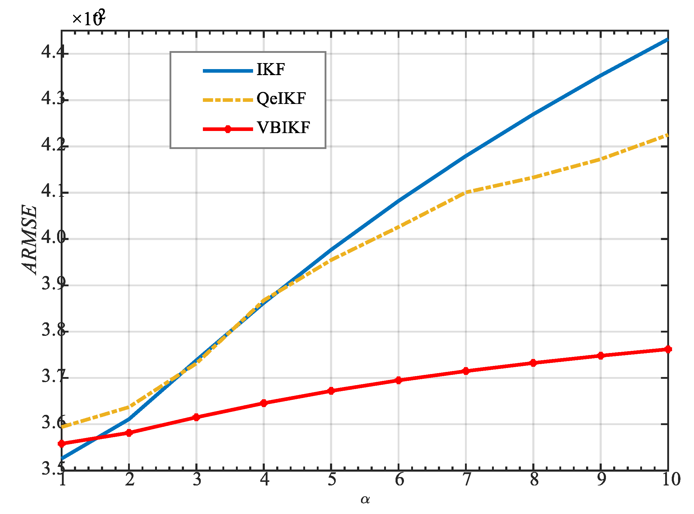
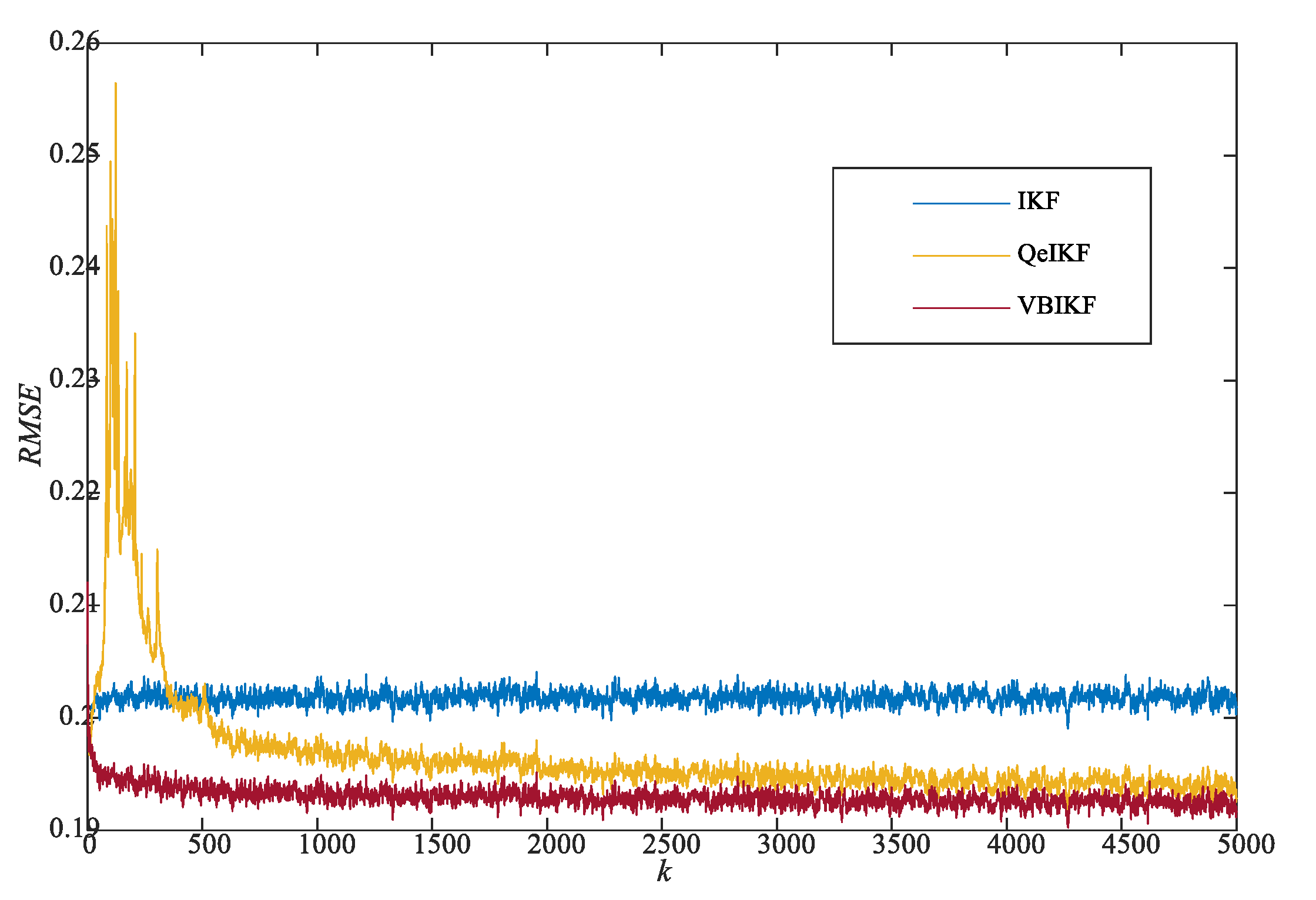
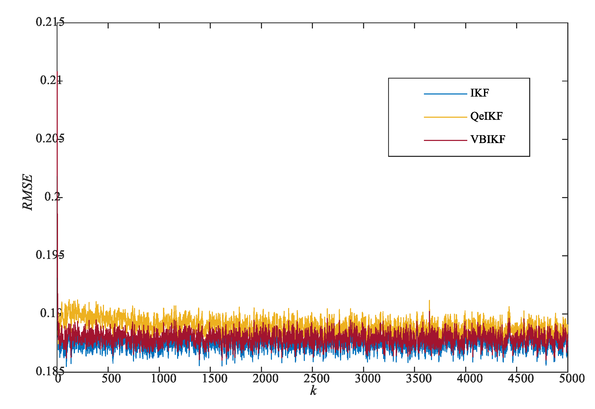
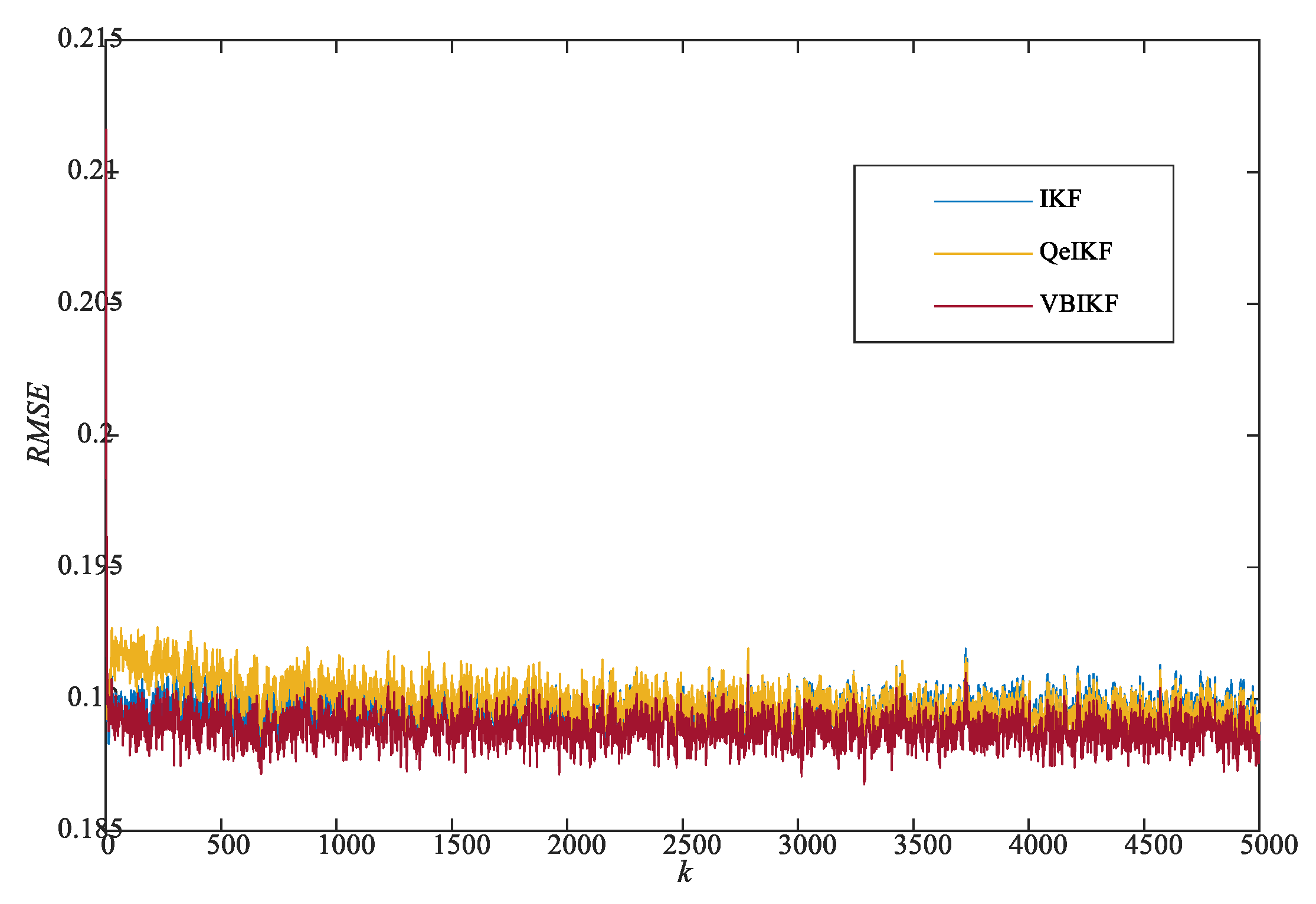
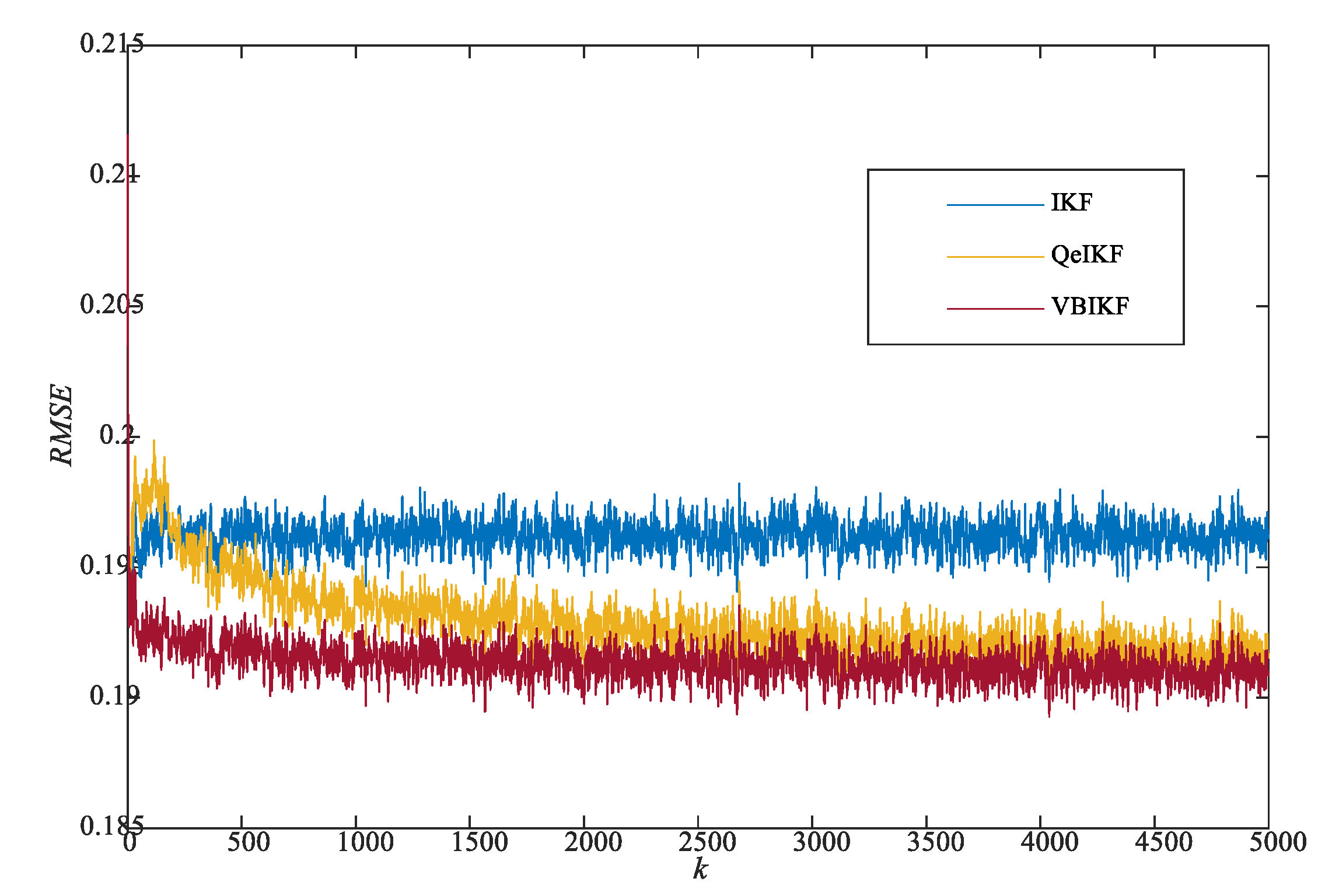
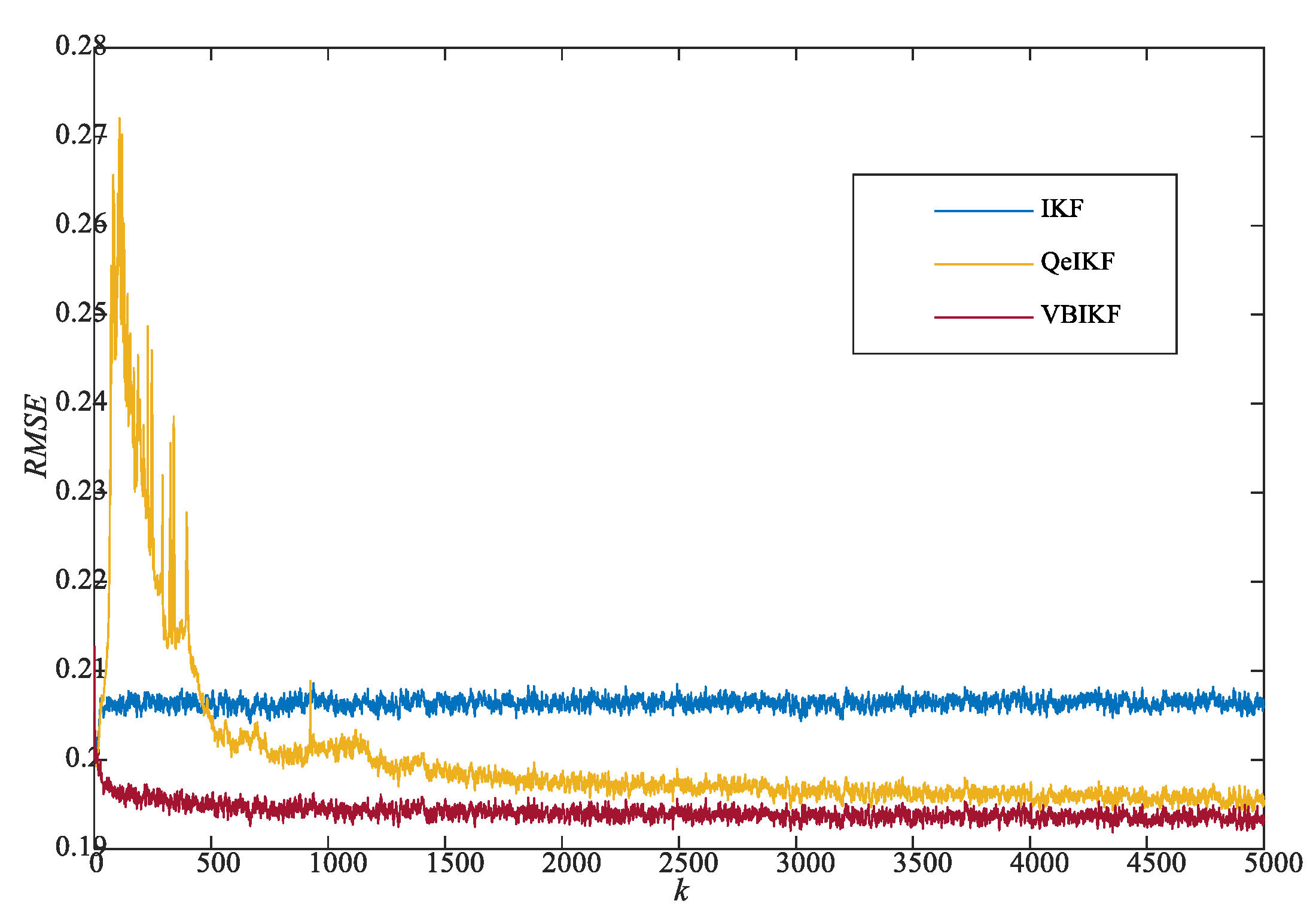
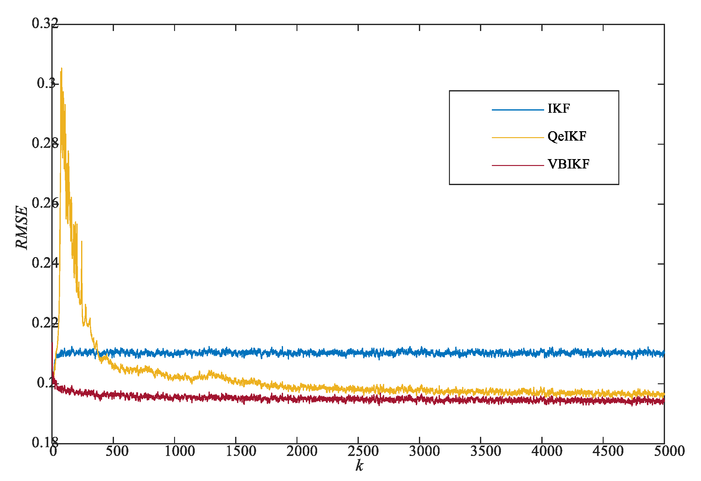
For all cases of the biased ${\widehat{\Sigma }}_w$ with $\alpha \ne$ 1, the presented ARMSE and $RMS{E}_k$ data clearly demonstrate that the proposed VBIKF not only shows better filtering precision than the QeIKF but its filtering stability is obviously superior to that of QeIKF;

(3)

Note that, for the biased ${\widehat{\Sigma }}_w$ with different $\alpha$, although the ARMSE of the proposed VBIKF is still influenced to some extent (i.e., the higher ARMSE value 0.0376 for $\alpha$ = 10), the negative influence caused by the inaccurate ${\widehat{\Sigma }}_w$ is significantly reduced compared with and smaller than the 0.0422 of the QeIKF and the 0.443 of the IKF;

(4)

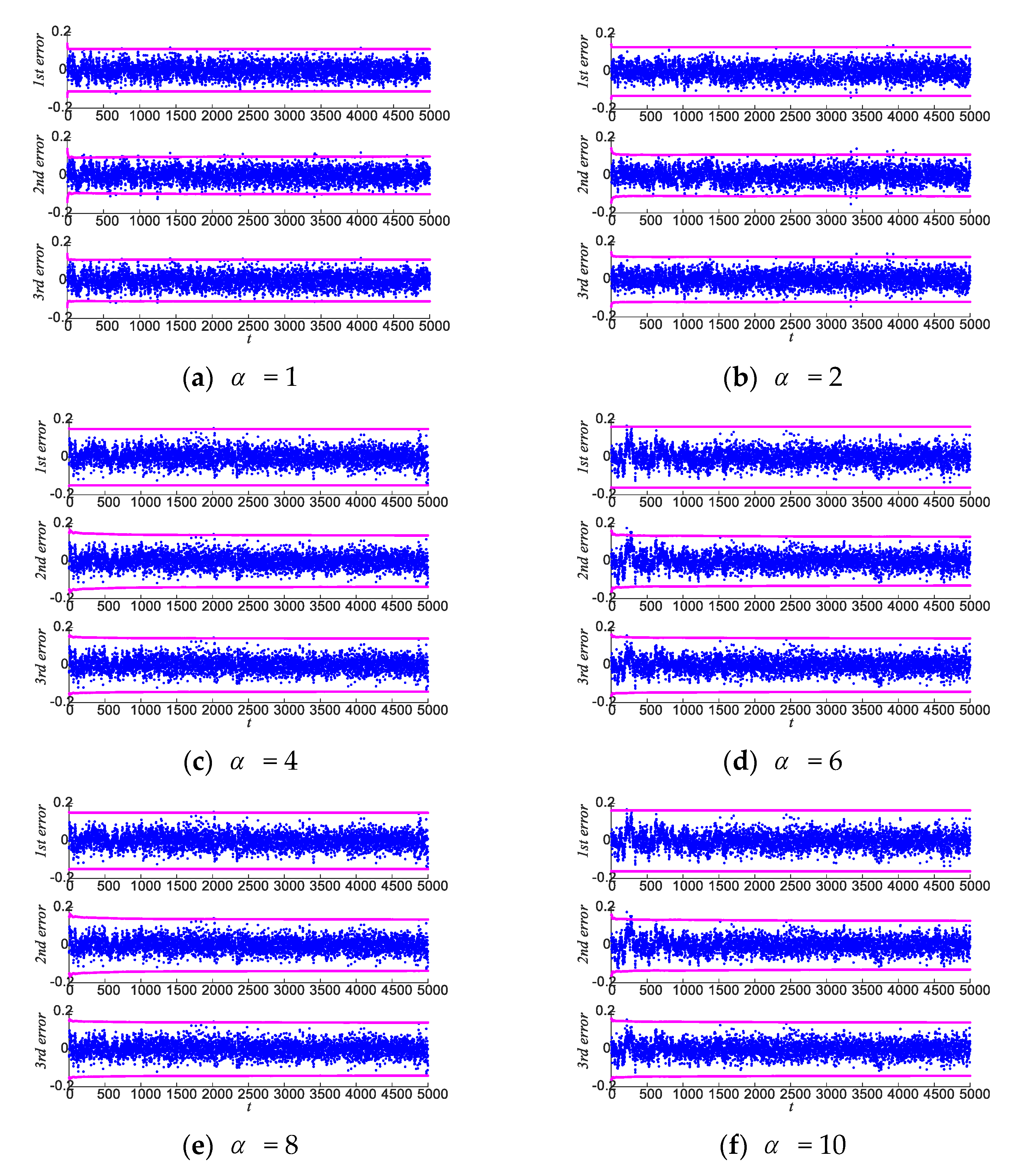
The respective errors of three elements of ${\xi }_k$ with the corresponding 3 $\sigma$ boundary for the VBIKF are presented in Figure 8 using the scaled ${\widehat{\Sigma }}_w$ with $\alpha$ = 1, 2, 4, 6, 8, and 10, which clearly shows that most of the time estimation errors would fall within the 3 $\sigma$ boundary.

(5)

As to the computational cost, the usage of extra fixed-point iterations introduces a longer running time than that of the conventional methods. For example, in this work the iteration number N was set to 8 and the average running time was about 6 times that of the conventional IKF. Obviously, an N that is too large is sure to increase the computational cost of the algorithm’s implementation and so a balance between precision and cost should be considered according to the particular application.

As to the ARMSE result displayed in Figure 1 and Table 1, if the scale parameter $\alpha$ is close or equal to 1 ($\alpha$ = 1), the employed covariance ${\widehat{\Sigma }}_w$ is close to its true ${\Sigma }_w$. Then, the ARMSE value of the standard IKF is the lowest among the three methods and its performance is optimal in the least square sense, which is also certified by the data on $RMS{E}_k$ displayed in Figure 2. However, when $\alpha$ becomes larger (for instance, $\alpha \ge$ 2), the accuracy of the employed ${\widehat{\Sigma }}_w$ is biased by the scaling parameter $\alpha$ and the ARMSE value of the IKF increases significantly, which means that the optimal estimation performance of the IKF is destroyed by the inaccurate ${\widehat{\Sigma }}_w$. We can conclude that the performance of the IKF is rather sensitive to the accuracy of ${\widehat{\Sigma }}_w$ and, for cases of an inaccurate ${\widehat{\Sigma }}_w$, adaptive methods are necessary to improve the performance of attitude estimation.

Note that the ARMSE result of the QeIKF shows some adaptability to the inaccurate ${\widehat{\Sigma }}_w$ with $\alpha >4$, which can also be verified by the data on $RMS{E}_k$ in Figure 4, Figure 5, Figure 6 and Figure 7; however, the estimation precision is still degraded by the inaccurate parameter and its effective range is limited. For the cases of $\alpha >6$, the estimation precision is still degraded by the inaccurate parameter and its effective range is rather small and limited. Moreover, as the $RMS{E}_k$ data show in Figure 5, Figure 6 and Figure 7, the process data on the QeIKF show some instability during the initializing stage; in fact, the critical issue with the QeIKF is that its filtering is not stable and rather prone to divergence [28]. In conclusion, the filtering precision and stability of the available QeIKF could not effectively reduce the influence of the inaccurate ${\widehat{\Sigma }}_w$.

5. Conclusions

For aerospace, satellite, and robotics engineering, the matrix Lie group attitude estimation problem with an inaccurate process noise covariance was investigated and a variational Bayesian iteration-based adaptive invariant Kalman filter (VBIKF) was proposed. In the VBIKF, the a priori error covariance is not propagated by the conventional steps but directly calibrated in an iterative manner based on the posterior sequences. The main advantage is that the statistics parameter of the system process noise is no longer required such that the IKF’s hard dependency on accurate process noise statistics can be reduced significantly. The numerical simulation results presented demonstrate the superior performance of the proposed VBIKF in terms of filtering adaptability and simplicity.

References

- Wu, J.; Shan, S. Dot Product Equality Constrained Attitude Determination from Two Vector Observations: Theory and Astronautical Applications. Aerospace 2019, 6, 102. [Google Scholar] [CrossRef] [Green Version]
- Phisannupawong, T.; Kamsing, P.; Torteeka, P.; Channumsin, S.; Sawangwit, U.; Hematulin, W.; Jarawan, T.; Somjit, T.; Yooyen, S.; Delahaye, D.; et al. Vision-Based Spacecraft Pose Estimation via a Deep Convolutional Neural Network for Noncooperative Docking Operations. Aerospace 2020, 7, 126. [Google Scholar] [CrossRef]
- Louédec, M.; Jaulin, L. Interval Extended Kalman Filter-Application to Underwater Localization and Control. Algorithms 2021, 14, 142. [Google Scholar] [CrossRef]
- Soken, H.E.; Sakai, S.-I.; Asamura, K.; Nakamura, Y.; Takashima, T.; Shinohara, I. Filtering-Based Three-Axis Attitude Determination Package for Spinning Spacecraft: Preliminary Results with Arase. Aerospace 2020, 7, 97. [Google Scholar] [CrossRef]
- Li, J.; Wei, X.; Zhang, G. An Extended Kalman Filter-Based Attitude Tracking Algorithm for Star Sensors. Sensors 2017, 17, 1921. [Google Scholar] [CrossRef] [Green Version]
- Pan, C.; Qian, N.; Li, Z.; Gao, J.; Liu, Z.; Shao, K. A Robust Adaptive Cubature Kalman Filter Based on SVD for Dual-Antenna GNSS/MIMU Tightly Coupled Integration. Remote Sens. 2021, 13, 1943. [Google Scholar] [CrossRef]
- Zheng, L.; Zhan, X.; Zhang, X. Nonlinear Complementary Filter for Attitude Estimation by Fusing Inertial Sensors and a Camera. Sensors 2020, 20, 6752. [Google Scholar] [CrossRef]
- Ayala, V.; Román-Flores, H.; Torreblanca Todco, M.; Zapana, E. Observability and Symmetries of Linear Control Systems. Symmetry 2020, 12, 953. [Google Scholar] [CrossRef]
- Deibe, Á.; Antón Nacimiento, J.A.; Cardenal, J.; López Peña, F. A Kalman Filter for Nonlinear Attitude Estimation Using Time Variable Matrices and Quaternions. Sensors 2020, 20, 6731. [Google Scholar] [CrossRef]
- Guo, H.; Liu, H.; Hu, X.; Zhou, Y. A Global Interconnected Observer for Attitude and Gyro Bias Estimation with Vector Measurements. Sensors 2020, 20, 6514. [Google Scholar] [CrossRef]
- Chaturvedi, N.; Sanyal, A.; Mcclamroch, A. Rigid-body attitude control using rotation matrices for continuous singularity-free control laws. IEEE Control Syst. Mag. 2011, 31, 30–51. [Google Scholar]
- Bonnabel, S.; Martin, P.; Salaun, E. Invariant Extended Kalman Filter: Theory and application to a velocity-aided attitude estimation problem. In Proceedings of the 48th IEEE Conference on Decision and Control (CDC) Held jointly with 2009 28th Chinese Control Conference, Shanghai, China, 15–18 December 2009. [Google Scholar] [CrossRef] [Green Version]
- Vasconcelos, J.; Cunha, R.; Silvestre, C.; Oliveira, P. A nonlinear position and attitude observer on SE(3) using landmark measurements. Syst. Control Lett. 2010, 59, 155–166. [Google Scholar] [CrossRef]
- Barrau, A.; Bonnabel, S. Intrinsic filtering on Lie groups with applications to attitude estimation. IEEE Trans. Autom. Contr. 2014, 60, 436–449. [Google Scholar] [CrossRef]
- Barrau, A.; Bonnabel, S. The invariant extended Kalman filter as a stable observer. IEEE Trans. Autom. Contr. 2017, 62, 1797–1812. [Google Scholar] [CrossRef] [Green Version]
- Barrau, A.; Bonnabel, S. Invariant Kalman filtering. Annu. Rev. Control Robot. Auton. Syst. 2018, 1, 237–257. [Google Scholar] [CrossRef]
- Batista, P.; Silvestre, C.; Oliveira, P. A GES attitude observer with single vector observations. Automatica 2012, 49, 388–395. [Google Scholar] [CrossRef]
- Chirikjian, G.; Kobilarov, M. Gaussian approximation of non-linear measurement models on lie groups. In Proceedings of the IEEE Conference on Decision and Control, Osaka, Japan, 15–18 December 2015. [Google Scholar]
- Barfoot, T.; Furgale, P. Associating uncertainty with three-dimensional poses for use in estimation problems. IEEE Trans. Robot. 2014, 30, 679–693. [Google Scholar] [CrossRef]
- Said, S.; Manton, J. Extrinsic mean of Brownian distributions on compact lie groups. IEEE Trans. Inf. Theory 2012, 58, 3521–3535. [Google Scholar] [CrossRef] [Green Version]
- Karasalo, M.; Hu, X. An optimization approach to adaptive Kalman filtering. Automatica 2011, 47, 1785–1793. [Google Scholar] [CrossRef] [Green Version]
- Wang, J.; Wang, J.; Zhang, D.; Shao, X.; Chen, G. Kalman filtering through the feedback adaption of prior error covariance. Signal Process. 2018, 152, 47–53. [Google Scholar] [CrossRef]
- Feng, B.; Fu, M.; Ma, H.; Xia, Y.; Wang, B. Kalman filter with recursive covariance Estimation-sequentially estimating process noise covariance. IEEE Trans. Ind. Electron. 2014, 61, 6253–6263. [Google Scholar] [CrossRef]
- Zanni, L.; Le Boudec, J.; Cherkaoui, R.; Paolone, M. A prediction-error covariance estimator for adaptive Kalman filtering in step-varying processes: Application to power-system state estimation. IEEE Trans. Contr. Syst. Technol. 2017, 25, 1683–1697. [Google Scholar] [CrossRef] [Green Version]
- Mohamed, A.; Schwarz, K. Adaptive Kalman Filtering for INS/GPS. J. Geod. 1999, 73, 193–203. [Google Scholar] [CrossRef]
- Ardeshiri, T.; Özkan, E.; Orguner, U.; Gustafsson, F. Approximate Bayesian smoothing with unknown process and measurement noise covariance. IEEE Signal Process. Lett. 2015, 22, 2450–2454. [Google Scholar] [CrossRef] [Green Version]
- Assa, A.; Plataniotinos, K. Adptive Kalman filtering by covariance sampling. IEEE Signal Process. Lett. 2017, 24, 1288–1292. [Google Scholar] [CrossRef]
- Huang, Y.; Zhang, Y.; Wu, Z.; Li, N.; Chambers, J. A novel adaptive Kalman filter with inaccurate process and measurement noise covariance matrices. IEEE Trans. Autom. Contr. 2018, 63, 594–601. [Google Scholar] [CrossRef] [Green Version]
- Ćesić, J.; Markovi, I.; Petrovi, I. Mixture Reduction on Matrix Lie Groups. IEEE Signal Process. Lett. 2017, 24, 1719–1723. [Google Scholar] [CrossRef] [Green Version]
- Ćesić, J.; Markovi, I.; Bukal, M.; Petrović, I. Extended Information Filter on Matrix Lie Groups. Automatica 2017, 82, 226–234. [Google Scholar] [CrossRef]
- Kang, D.; Jang, C.; Park, F. Unscented Kalman Filtering for Simultaneous Estimation of Attitude and Gyroscope Bias. IEEE/ASME Trans. Mechatron. 2019, 24, 350–360. [Google Scholar] [CrossRef]
- Bourmaud, G.; Mégret, R.; Arnaudon, M.; Giremus, A. Continuous-Discrete Extended Kalman Filter on Matrix Lie Groups Using Concentrated Gaussian Distributions. J. Math. Imaging Vis. 2015, 51, 209–228. [Google Scholar] [CrossRef] [Green Version]
- Tzikas, D.; Likas, A.; Galatsanos, N. The Variational Approximation for Bayesian Inference. IEEE Signal Process. Mag. 2008, 25, 131–146. [Google Scholar] [CrossRef]