Article

Unscented Kalman Filter-Aided Long Short-Term Memory Approach for Wind Nowcasting

1
School of Computational Science and Engineering, Georgia Institute of Technology, Atlanta, GA 30332, USA
2
Department of Robot and Smart System Engineering, Kyungpook National University, Daegu 41566, Korea
*
Author to whom correspondence should be addressed.
Aerospace 2021, 8(9), 236; https://doi.org/10.3390/aerospace8090236
Submission received: 25 May 2021 / Revised: 21 August 2021 / Accepted: 24 August 2021 / Published: 26 August 2021
(This article belongs to the Special Issue Application of Data Science to Aviation)

Abstract

:
Obtaining reliable wind information is critical for efficiently managing air traffic and airport operations. Wind forecasting has been considered one of the most challenging tasks in the aviation industry. Recently, with the advent of artificial intelligence, many machine learning techniques have been widely used to address a variety of complex phenomena in wind predictions. In this paper, we propose a hybrid framework that combines a machine learning model with Kalman filtering for a wind nowcasting problem in the aviation industry. More specifically, this study has three objectives as follows: (1) compare the performance of the machine learning models (i.e., Gaussian process, multi-layer perceptron, and long short-term memory (LSTM) network) to identify the most appropriate model for wind predictions, (2) combine the machine learning model selected in step (1) with an unscented Kalman filter (UKF) to improve the fidelity of the model, and (3) perform Monte Carlo simulations to quantify uncertainties arising from the modeling process. Results show that short-term time-series wind datasets are best predicted by the LSTM network compared to the other machine learning models and the UKF-aided LSTM (UKF-LSTM) approach outperforms the LSTM network only, especially when long-term wind forecasting needs to be considered.

1. Introduction

According to the Federal Aviation Administration (FAA), the FAA’s air traffic organization served more than 44,000 flights and 2.7 million airline passengers daily in over 29 million square miles of airspace before the COVID-19 pandemic [1]. This is already a large number of flights and passengers; however, the FAA expects the United States (U.S.) domestic carrier passenger growth to average 1.8 percent per year over the next 20 years [2]. As aviation traffic continues to grow, most airport operators are concerned about ground delays directly related to operating costs [3]. Among various factors that affect the ground delays, accurate wind information around an airport is the most significant factor in evaluating the efficiency of airport operations [4]. Wind forecasting has recently been recognized as one of the most challenging tasks in the aviation industry [5].
Many research groups have been dedicated to developing numerical weather models to predict weather patterns. The two best known numerical weather models are the Global Forecast System [6] developed by the the National Oceanic and Atmospheric Administration (NOAA) and the European Centre for Medium-Range Weather Forecasts [7] developed by the European Centre, which are called the American model and the European model, respectively. While numerical weather models have been widely used in the aviation industry, it is worth mentioning that numerical weather models have some limitations in predicting wind patterns due to aleatory uncertainty. Recently, many machine learning techniques have been used along with a myriad of data-driven approaches to enhance the level of understanding of various complex phenomena in nature such as wind predictions.
In this paper, we propose a hybrid framework that combines a machine learning model and a Kalman filtering technique for a wind nowcasting problem in the aviation industry. More specifically, this research has three goals as follows: (1) compare machine learning models (i.e., Gaussian process (GP), multi-layer perceptron (MLP), and long short-term memory (LSTM) network [8]) to identify the most suitable model for wind predictions in Section 3.5, (2) combine the machine learning model selected in step (1) with an unscented Kalman filter (UKF) [9] to improve the fidelity of the model in Section 3.6, and (3) perform Monte Carlo simulations (MCSs) to quantify uncertainties arising from each modeling process in Section 3.7.
For the data-driven wind nowcasting approach proposed in this paper, we utilize the Modern-Era Retrospective analysis for Research and Applications-2 (MERRA-2) dataset [10] provided by the National Aeronautics and Space Administration (NASA) given that the MERRA-2 wind dataset is widely used in the aviation industry. For example, the Aviation Environmental Design Tool [11] developed by the FAA utilizes MERRA-2 wind data to calculate fuel consumption in a simulation environment. However, even though the MERRA-2 dataset contains reliable wind information, it is important to note that the MERRA-2 wind dataset is not adequate for wind speed predictions as it is basically historical data. The main purpose of this research is to develop a hybrid framework (i.e., combination of a machine learning algorithm and Kalman filtering technique) that uses the MERRA-2 wind dataset for wind nowcasting in the aviation industry. The remainder of this paper contains the following sections: literature review (Section 2), proposed methodology (Section 3), results and discussion (Section 4), and conclusion (Section 5).

2. Related Work

With the advent of artificial intelligence (AI), many machine learning techniques have been widely used to address various and complex phenomena in nature. In particular, many researchers have proposed new approaches using machine learning techniques to predict wind speed information at a specific location. As an illustration, for wind speed predictions, Mohandes et al. [12] used the support vector machine and the MLP and Kulkarni et al. [13] compared the artificial neural network (ANN) model performance with several statistical regression methods. Furthermore, Rozas-Larraondo et al. [14] proposed a new method based on non-parametric multivariate locally weighted regression for wind speed forecasting in airports and Khosravi et al. [15] conducted a case study to compare machine learning algorithms for time-series wind speed prediction at a wind farm in Brazil. Recently, various versions of the LSTM network have been widely used for short-term wind speed predictions [16,17,18].
Although machine learning techniques generally outperform traditional approaches (e.g., numerical weather models) in wind predictions, they do not always provide accurate wind information due to unpredictable uncertainties. In some cases, machine learning techniques are combined in a hybrid approach to provide more accurate wind predictions. For instance, for short-term wind speed predictions, extreme learning machines [19] are combined with either the nearest neighbors approach [20], the adaptive noise and auto-regressive integrated moving average approach [21], or the improved seagull optimization algorithm [22]. Furthermore, Nezhad et al. [23] developed a new combined model that integrates wind source potential assessment and forecasting using image processing of satellite data and an adaptive neuro-fuzzy inference system. In 2021, Imani et al. [24] combined the rough and fuzzy set theory in the LSTM model to enhance accuracy and reduce data uncertainties.
Although the aforementioned hybrid methods improved the accuracy of short-term wind predictions, they might not be suitable frameworks for long-term wind forecasting since they did not use current and in-site measurements unlike Kalman filtering. In other words, it has been recently found that Kalman filtering [25,26] can improve the fidelity of machine learning models. As an illustration, Lee and Johnson [27] showed that Kalman filtering improves the accuracy of machine learning models such as GP regression and Ullah et al. [28] proposed a hybrid method combining an ANN and a Kalman filter technique to improve the performance of a prediction algorithm under dynamic conditions. In addition, Hur [29] recently presented a wind speed prediction scheme that comprises two stages: estimation by an extended Kalman filter (EKF) and prediction by a neural network. While the aforementioned literature survey has demonstrated the capability for wind forecasting, the proposed methods may not be applicable for the MERRA-2 wind dataset, which is one of the most commonly used wind datasets in the aviation industry, as the methods were not trained and developed using the MERRA-2 dataset. It is also worth mentioning that the methods did not consider a validation process at aviation-related locations such as cruise points of aircraft. Thus, the main contribution of this paper is to develop a hybrid framework that combines a machine learning model with Kalman filtering for wind nowcasting, especially using MERRA-2 wind data.

3. Methodology

This paper aims to develop a framework that performs wind nowcasting by combining a machine learning model with a Kalman filtering technique. The framework proposed in this paper consists of four phases as follows: (1) decompose annual wind data into training and validation samples as described in Section 3.1, (2) compare machine learning models (i.e., MLP, GP, and LSTM) to identify the most appropriate model for wind predictions as presented in Section 3.5, (3) combine the selected machine learning model with a UKF to improve the fidelity of the model as presented in Section 3.6, and (4) perform MCSs to quantify uncertainties arising from the modeling processes as described in Section 3.7. Figure 1 delineates an overall flowchart of the proposed framework.

3.1. Data Preparation

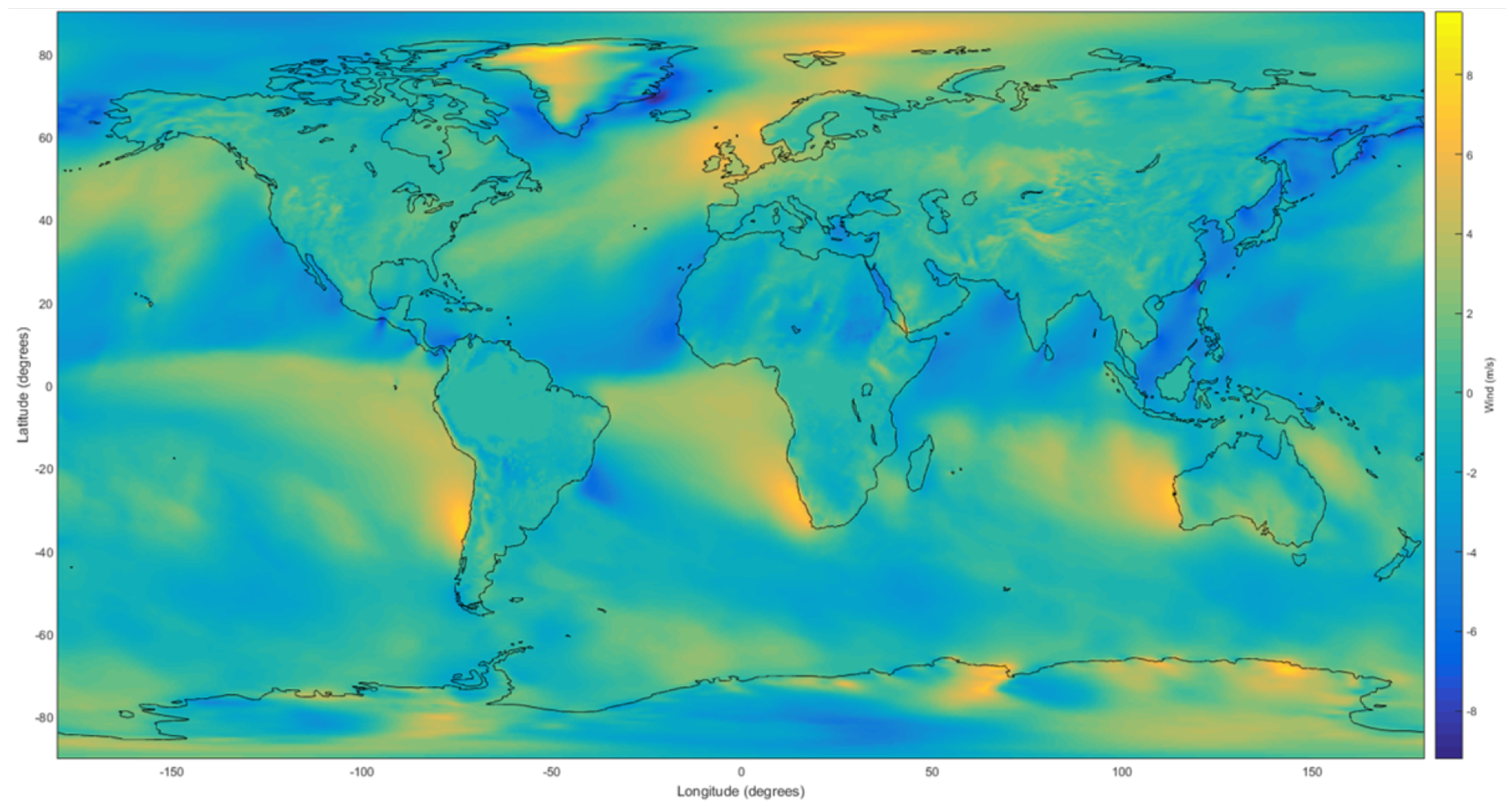
MERRA-2 contains a set of detailed weather-related properties (e.g., wind, humidity, and temperature) against longitude, latitude, altitude, and timestamp. Among various MERRA-2 weather variables, we specifically collected eastward and northward wind speed data as we wanted to develop a framework that performs wind predictions (e.g., eastward wind model and northward wind model) with the aim of providing an accurate wind forecast to the aviation industry. Figure 2 shows an example visualization of the MERRA-2 winds at a certain time and altitude.
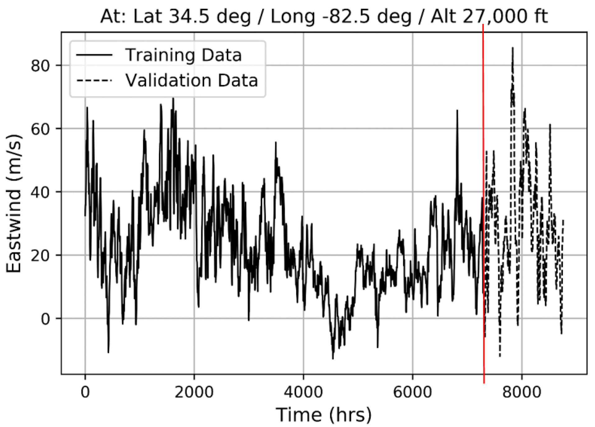
In terms of time-series data preparation, we retrieved the MERRA-2 wind dataset (i.e., three-hour interval dataset) from January to December in 2018 at a point of interest. To specify the point of interest, we collected the previous Delta Airlines 2638 flight trajectory information through the FlightAware flight tracking data platform [30]. We then selected one of the points consisting of the cruise phase of the flight (i.e., altitude = 34,000 feet). As the next step, we collected wind information at the point of interest from January to December in 2018 and generated a CSV file that includes information with respect to date and wind speed. Additionally, we decomposed the time-series dataset into a training (84%) phase (i.e., from January to October) and a validation (16%) phase (i.e., from November to December) for a holdout validation purpose. Figure 3 shows how the MERRA-2 annual wind datasets are decomposed into training and validation phases.
Mathematically, given N number of data samples, we generated a dataset of N 1 input and output pairs by shifting each data point for one-step-ahead forecasting; thus, the inputs become x 1 : N 1 and their corresponding outputs are x 2 : N . Here, subscript 1 : N means the history of the data from discrete time 1 to time N. In a nutshell, given the set of training data D = x 1 : N 1 , x 2 : N , a machine learning model identifies the relationship between input x i 1 and output x i by predicting output x i + 1 with new input point x i . Here, we model wind speed information with one-step-ahead forecasting because the overall framework proposed in this paper includes the Kalman filter technique that generally follows one-step-ahead propagation [25]. The discrete dynamic equation of each wind is defined as follows:
x i = f ( x i 1 , η i 1 ) ,
where f ( · ) is wind dynamics that will be modeled by a machine learning technique and η is white noise. Here, x is an accessible ground-truth value (i.e., MERRA-2 wind data in this paper) in training and validation phases. It is important to note that we concentrated only on the point of interest to validate the applicability of the proposed methodology and further investigations may be conducted at other locations in U.S. territories (e.g., weather stations) when necessary.

3.2. Gaussian Process (GP)

A GP, which is also known as Kriging, was originally introduced by Matheron [31] as a geostatistical estimation method. The GP has been widely utilized in general regression problems because of the advantage that its prediction is probabilistic in such a way that it provides uncertainty bounds of the predictions. In this paper, we implemented the GP to create a nonlinear probabilistic regression model of MERRA-2 wind data. Given N input and output pairs, the hyper-parameters of the kernel were optimized during the GP regression process by maximizing the log marginal likelihood of the outputs. Additional details are summarized in Appendix A.

3.3. Multi-Layer Perceptron (MLP)

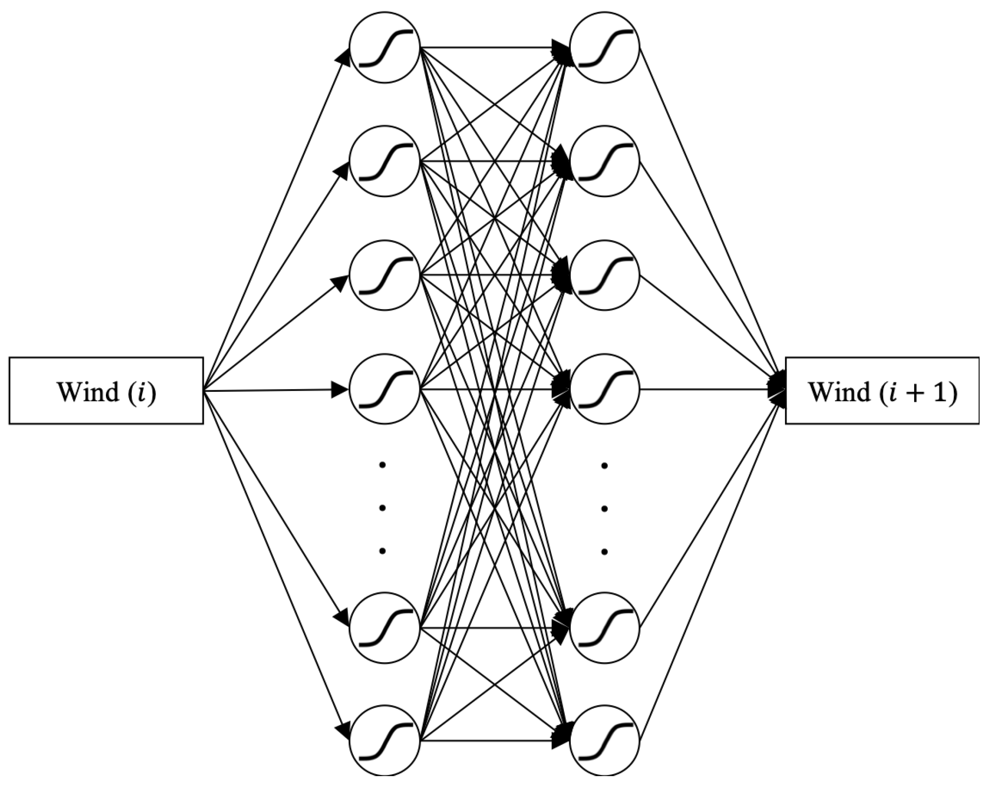
We implemented the MLP to create a nonlinear regression model of MERRA-2 wind data with the aim of finding the best weight parameters to minimize errors between predicted and target values. To find the best weight parameters in the model, we utilized the Adam algorithm that is an extended version of the stochastic gradient descent method. The MLP-based wind regression model entails the following fully-connected layers: (1) an input layer to receive MERRA-2 wind data, (2) an output layer with the linear activation function that makes a prediction, and (3) two hidden layers with the sigmoid function. Figure 4 shows the diagram of the MLP model structure used for this paper. To isolate the free hyper-parameters of the MLP wind regression model, we formulated the design of experiment (DoE) with respect to a number of hidden layers, a number of hidden nodes, learning rate, regularization penalty parameter, and batch size. The effective MLP model was finally determined by the choice of hyper-parameters tabulated in Table 1.

3.4. Long Short-Term Memory (LSTM) Network

While the MLP is widely used for nonlinear regression problems, it is important to note that the MLP-based regression method may not be robust for solving complex problems that frequently appear in nature. For this reason, many AI researchers have been committed to developing deep learning (DL) models that are generally defined with more than two hidden layers without losing the key idea of the MLP technique. The recurrent neural network (RNN), which is one of the DL models devised by mimicking the sequential processes of the human brain, has been introduced to particularly deal with time-series prediction tasks by allowing information to persist in network loops. However, one potential issue is that the RNN may not be capable of handling long-term dependencies, indicating that it only works well if the gap between previous and present information is small. In response to this concern, the LSTM network [8] was introduced to specifically handle long-term dependencies. The LSTM network typically has a memory block (i.e., output gate, input gate, forget gate) interacting in a very special way in modules. In this paper, we implemented the LSTM network, one of the popular DL models especially for time-series predictions, to handle sequential MERRA-2 wind data. That is, the LSTM network models true wind dynamics f ( · ) described in Equation (1), resulting in f LSTM ( · ) as follows:
x ^ i = f LSTM ( x i 1 ) ,
where x i 1 is the ground truth value at time ( i 1 ) and x ^ i is a predicted value at time i. In particular, we used the Keras LSTM library [32] to perform wind predictions with MERRA-2 data. The LSTM model structure used for this paper was constructed with the following properties as tabulated in Table 2.

3.5. Model Evaluation and Comparison

To identify the most appropriate machine-learning-based time-series wind prediction model, we computed the coefficient of determination (i.e., R-squared), root-mean-square error (RMSE), and mean absolute error (MAE) [33] with respect to the validation dataset. The error metrics used in this paper are defined as follows:
RMSE = 1 M i = 1 M | x i x ^ i | 2 MAE = 1 M i = 1 M | x i x ^ i | ,
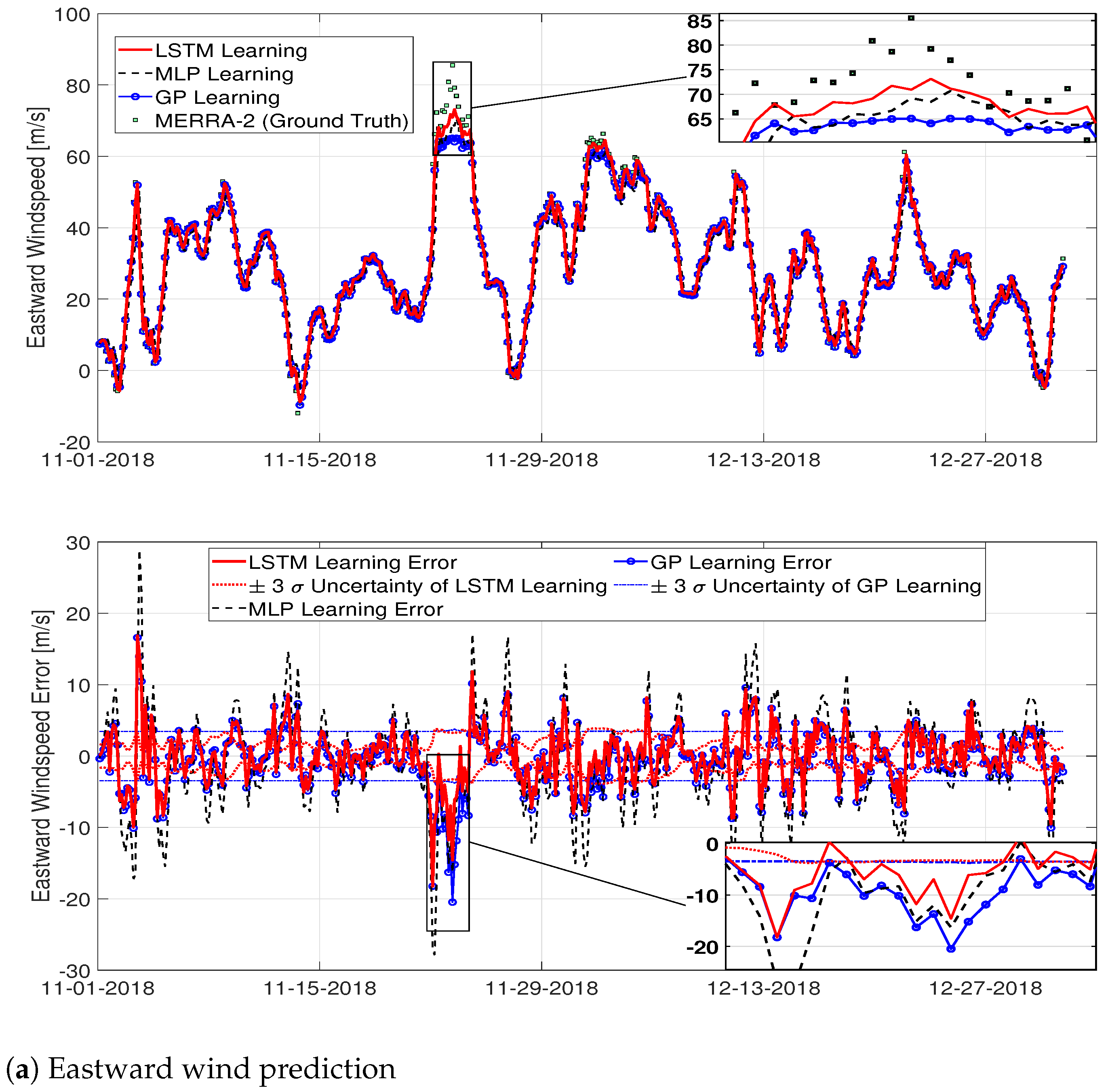
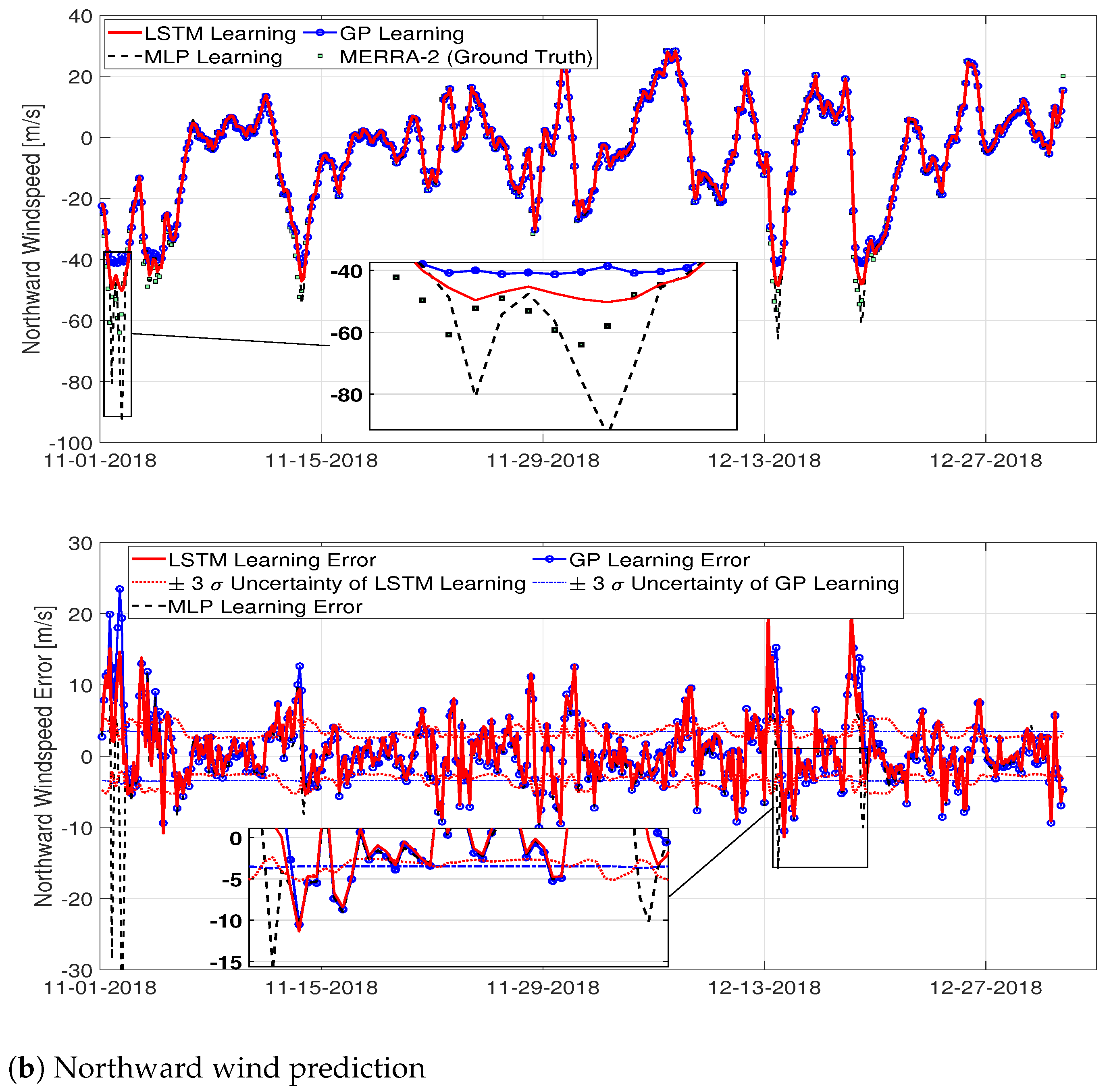
where M is the number of data for this validation phase. The results are tabulated in Table 3. We also calculated the prediction errors ( = x ^ i x i ) and uncertainty bounds of the models as shown in Figure 5. The results from Table 3 and Figure 5 indicate that time-series wind datasets are best predicted by the LSTM network (e.g., smallest RMSE and MAE) compared to the other machine learning models (i.e., GP and MLP).

3.6. UKF-Aided LSTM (UKF-LSTM) Approach

The most widely used algorithm for estimating the state variables of a dynamic system is a Kalman filter [25,26]. The Kalman filtering framework consists of two steps: (1) time update and (2) measurement update. In the step of time update (i.e., state propagation), it predicts state variables (e.g., wind speed in this paper) from one discrete-time k to next time ( k + 1 ) , like the one-step-ahead prediction in Equation (1). Once measured sensor data at time ( k + 1 ) are incoming, the measurement-update step occurs. In the measurement update step, the filter corrects the predicted state value using predicted uncertainty based on RMSE minimization and recursive Bayesian estimation. In addition, to run the Kalman filter, the dynamic model and measurement model of the system are required to be known. When the model of the dynamic system is unknown or hard to be known (e.g., wind speed), we are able to use machine learning techniques to learn it. In fact, the machine learning community has applied machine learning techniques to both controls and estimation processes in the past. Estimation methods have ranged from Bayesian filtering with machine learning to nonlinear Kalman filtering with machine learning [27,34,35].
The Kalman filter is a linear quadratic estimator; thus, it performs only in linear systems. For handling nonlinear systems such as wind speed forecasting, we need to design nonlinear filters (e.g., EKF [36,37] and UKF [9]) modified from the linear Kalman filter. In this paper, we chose a UKF for the LSTM network selected for wind speed dynamics in Section 3.5. Since the LSTM network has no exact expression of analytical governing equations, obtaining the Jacobian of the LSTM network is challenging. Whereas an EKF requires computing Jacobian matrices, UKF does not since it is a more straightforward statistical approach. Moreover, theoretically, a UKF is more accurate than an EKF in nonlinear systems since the UKF has no linearization errors [38]. Although the UKF typically requires a high computational cost, the UKF has been selected for this research because the computational cost can be systematically manageable especially in the aviation domain. Mathematically, f LSTM ( · ) modeled in Equation (2) is used in the time update step as follows:
x ^ k + 1 = f LSTM ( x ^ k ) ,
where subscript k represents the k-th time step in the testing phase (i.e., long-term forecasting phase) and hat “ ^ ” denotes an estimate; state estimate x ^ : = E [ x ] . Superscript—represents an a priori estimate. Unlike Equation (2), ground truth is not accessible in the long-term forecasting phase, so the input of f LSTM ( · ) in Equation (3) is not x but x ^ . Initial condition x ( 0 ) = x 0 is given from the last point of the validation data (i.e., 21 UTC on December 31, 2018). In the step of measurement update:
x ^ k + 1 = x ^ k + 1 + Δ x ^ k + 1
Δ x ^ k + 1 = K k + 1 ( z ˜ k + 1 x ^ k + 1 ) ,
where optimal Kalman gain K is computed using predicted uncertainty and tilde “ ˜ ” denotes a measurement by a sensor. This measurement-update step is performed only when measurement data z ˜ are available in the filter. In other words, if there is no measurement in time ( k + 1 ) , there is no measurement-update step in Kalman filtering. That is, without a measurement at time ( k + 1 ) , there is no correction Δ x ^ k + 1 = 0 , and an a priori estimate is assigned to the final nowcasting at time ( k + 1 ) (i.e., x ^ k + 1 x ^ k + 1 ). For implementation, we used an open-sourced package of a UKF [39]. For more details of the UKF, see Appendix B.
Although it is possible to obtain more accurate data by averaging outputs from multiple high-accuracy sensors if the given time is not constrained, this is not practical. In practical applications in the aviation industry, a real-time sensor reading process typically generates random noise because the sensor is a cheap and easy-to-implement sensor. Hence, it is inevitable to fuse real-time noisy measurements into the estimate values especially when a wind nowcasting analysis is performed. In fact, we use simulated noisy measurements in this paper to focus on testing our UKF-LSTM framework since we do not have an actual sensor that measures real-time wind speed at a certain location for our experiments. In this paper, we assume that the simulated sensor rate is as fast as the time rate of the learned LSTM network. That is, whenever the time-update step in Equation (3) is performed, the measurement-update step (i.e., correction) in Equations (4) and (5) is assumed to be performed.
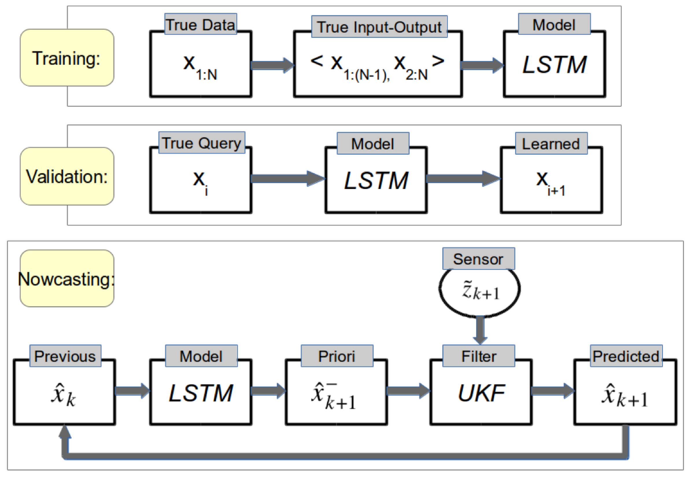
Figure 6 shows an overview of our methodology proposed in this paper. The proposed methodology consists of three phases (i.e., training, validation, and nowcasting) to predict wind speed information. We first decompose annual wind data points into N training and M validation samples. With N data points, we generate x 1 : N 1 input and x 2 : N output pairs by one-time shifting each point for preparing the training process. The training phase generates the LSTM network structure represented in Table 2. Next, the validation phase evaluates the performance of the trained LSTM model as illustrated in Table 3 and Figure 5. Once the LSTM model is validated, the nowcasting phase utilizes the UKF with sensor measurements (e.g., simulated noisy measurements in this paper) to improve the fidelity of the LSTM network. With the collaboration of the LSTM network and the UKF (i.e., UKF-LSTM), it eventually nowcasts wind values at each ( k + 1 ) timestamp.

3.7. Monte Carlo Simulation (MCS)-Based Uncertainty Quantification

It is important to quantify the various uncertainties arising from input data (e.g., aleatory uncertainty) or modeling processes (e.g., epistemic uncertainty), especially if there is a need to generate a predictive model using a supervised machine learning algorithm. An uncertainty bound is generally defined as an interval that consists of probabilistic upper and lower bounds on the estimate of outcomes generated from the predictive model. The uncertainty bound for a linear regression method can easily be calculated with given equations (i.e., prediction/confidence interval) [40]; however, it is challenging to compute an uncertainty bound for nonlinear regression techniques such as the MLP. While the GP can provide meaningful uncertainty bounds along with the training process where both the mean and covariance are designed to be computed (Appendix A), it is not possible for the LSTM network to directly calculate an uncertainty bound. For this reason, we performed the MCS, a technique used to illustrate the impact of uncertainty in forecasting models, to quantify uncertainties that could arise from the UKF-LSTM modeling process.
Even if a machine learning technique trains the same dataset, the hyper-parameters for the learned model could be different at each time due to the model uncertainty. For uncertainty quantification of the machine learning technique, we ran ten Monte Carlo trials. In other words, we generated ten machine learning models by applying one machine learning technique to the same data ten times and then we computed the mean and variance of the ten models. The mean and variance became the outcomes of the MCS as shown in Figure 5.
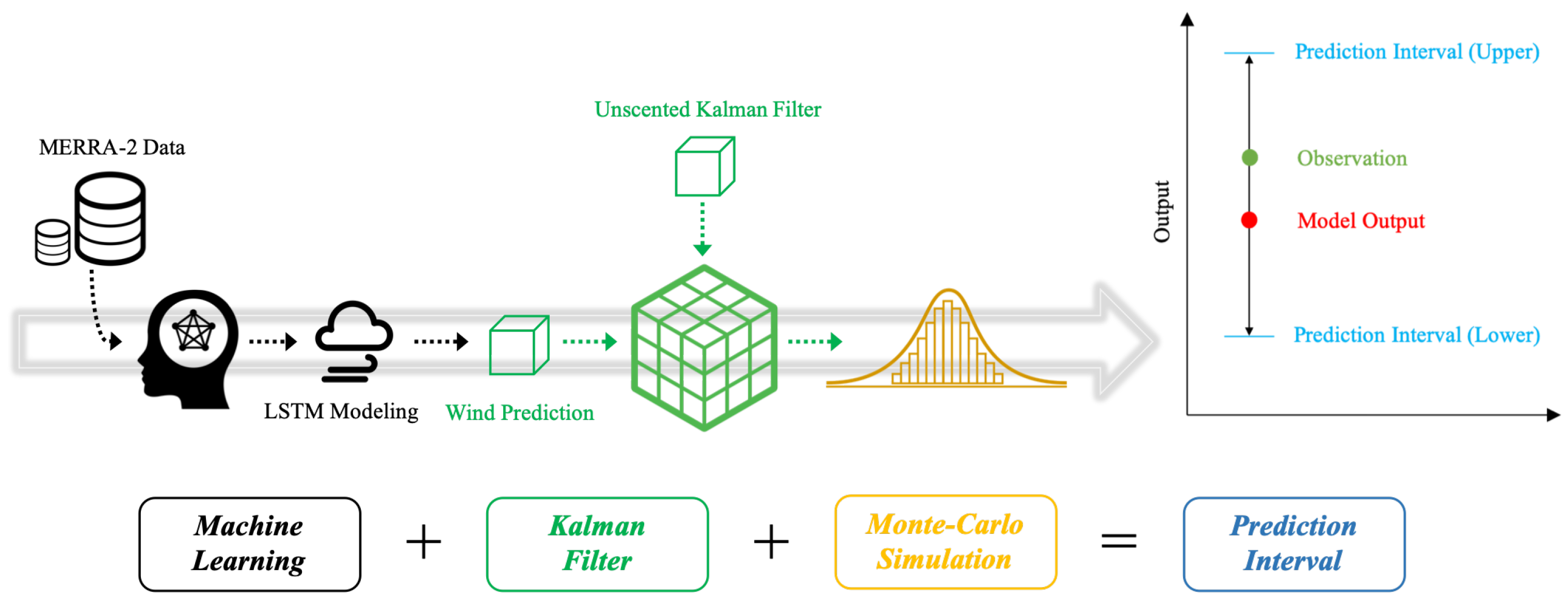
Since it was assumed that the UKF in the proposed framework uses an easy-to-implement sensor that typically generates random noise, we employed the Gaussian random walk to generate simulated measurement data in this paper. In other words, as the actual sensor hardware does not exist in the experiment of this study, within the scope of only validation of our framework, our sensor model used in the UKF comprised ground-truth values plus random noise. That is, in Equation (5), z ˜ k + 1 = x k + 1 + ζ k + 1 , where ζ is the Gaussian random measurement noise for the simulated measurement. Likewise, the simulated direct measurements were randomized, so we ran the MCS to quantify the uncertainty of our UKF-LSTM approach. More specifically, we conducted the following procedures to estimate an uncertainty bound of the UKF-LSTM process: (1) optimize hyper-parameters of the LSTM network, (2) generate ten distinct simulated measurements using ground truth (i.e., MERRA-2 wind), (3) run the UKF-LSTM ten times with the isolated hyper-parameters, and (4) compute the mean and variance to quantify an uncertainty bound. Figure 7 shows a notional sketch of the MCS-based uncertainty quantification process flowchart.

4. Results and Discussion

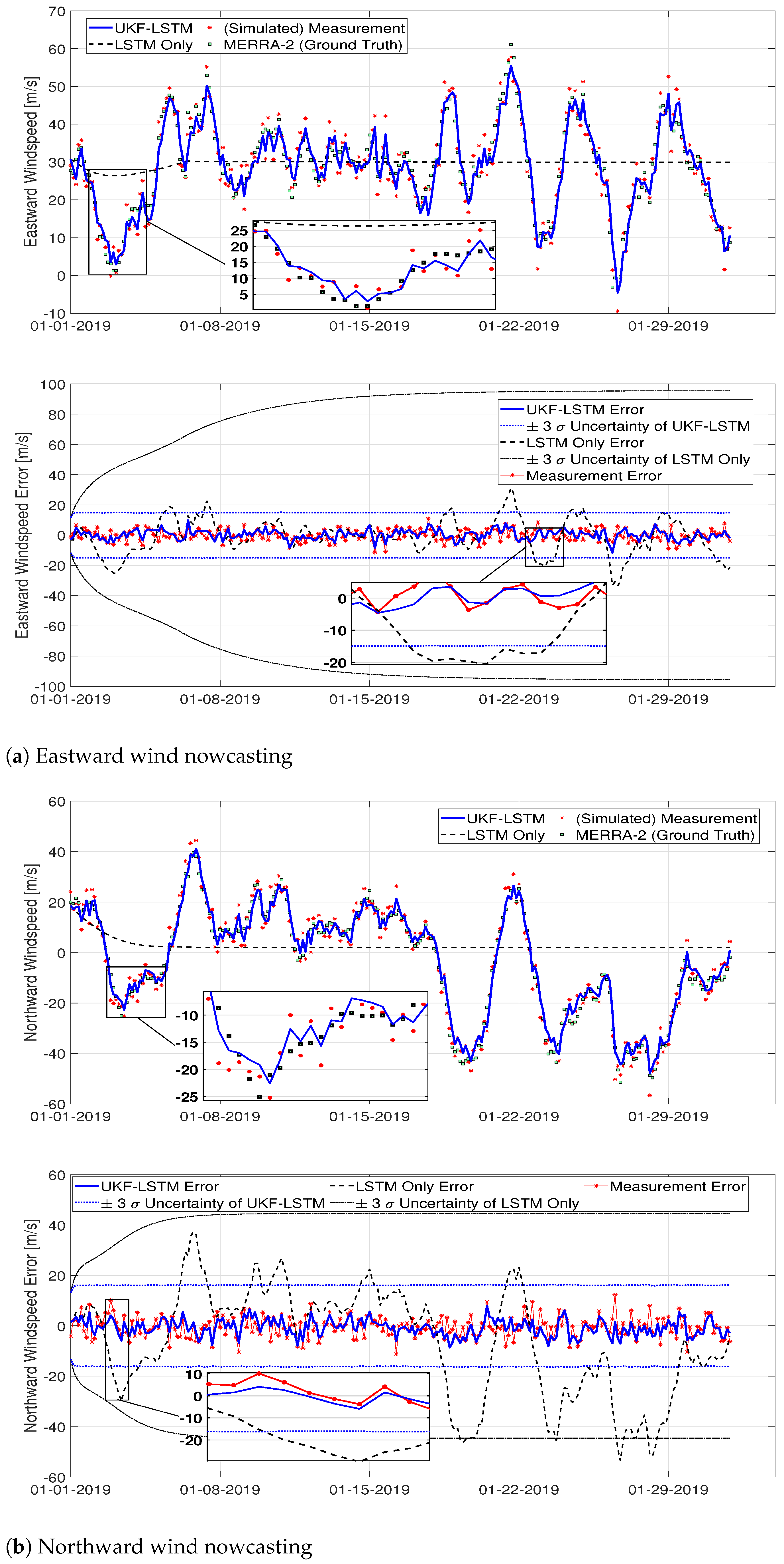
We went through the goodness-of-fit procedure for three different machine learning-based time-series wind prediction models that include the GP, the MLP, and the LSTM network to identify the most appropriate model for time-series wind forecasting. Figure 5 presents the following implications: (1) the prediction results from the LSTM network are much closer to the ground truth data (i.e., MERRA-2 wind data) than those from the other machine learning models (that is, the modeling error of the LSTM is the smallest), and (2) the uncertainty bound of the LSTM network is also smaller than the other uncertainty bound generated by the GP. In other words, the red solid line is more accurate than the black dashed line or the blue dash-circle line, indicating that the LSTM network is the most suitable machine learning technique that models the time-series wind dataset. It is worth mentioning that the validation process utilized validation datasets (i.e., MERRA-2 wind data) as an input for the models. After identifying the best model for time-series wind predictions (i.e., LSTM network) among three machine learning models, we combined the LSTM network with the UKF to improve the fidelity of the LSTM network. To compare the UKF-LSTM approach with the LSTM network, we utilized a testing dataset (i.e., January 2019) as the ground truth. In the testing phase, the ground-truth values are not accessible, and they are used only for evaluating the performance of the proposed framework. As shown in each top side of Figure 8, it was observed that UKF-LSTM provided a better wind prediction compared to the LSTM network, especially when long-term wind forecasting needs to be considered, while the LSTM network generated wind forecasts that are valid only for short-term predictions. Moreover, as shown in each bottom half of Figure 8, the errors of the UKF-LSTM are smaller than those of measurements represented as red asterisks, indicating that our approach is more accurate than measured values from a cheap sensor.
It is important to note that the LSTM network (i.e., LSTM network model without UKF) did not perform well for the testing dataset because the model used wind data predicted by the model in the previous step as an input (i.e., recursively predicted value), which potentially results in feeding relatively incorrect input data to the model; thus, the model error sequentially increased over time. In other words, unlike the proposed UKF-LSTM approach, the LSTM network used a priori estimate x ^ (i.e., values without the correction step described in Equation (4) as the input of f LSTM ( · ) in Equation (3). In fact, given that the MERRA-2 dataset does not provide wind forecasts in a timely manner but focuses more on providing historical data, this motivated us to develop the UKF-LSTM approach to resolve the issue by implementing a filtering process into the LSTM network. One may claim that the LSTM network with a rolling prediction [41] possibly forecasts over the long-term; however, we did not consider the approach in this paper because it would typically require a high computational cost, which may result in it not being applicable for wind nowcasting in the aviation industry.
To quantify uncertainties arising from the UKF-LSTM process, we performed the MCS with the isolated hyper-parameters of the LSTM network. As a result, the uncertainty bounds of the UKF-LSTM were identified, shown in each bottom half of Figure 8. As can be seen, it appears that the prediction error of the UKF-LSTM is within the uncertainty bound; thus, this indicates that the filtering process in our approach is well designed and well performed. However, it seems that the results of the LSTM network are averaged and its uncertainty is almost doubled compared to the UKF-LSTM approach. Moreover, the prediction error of the LSTM network is sometimes out of bounds; thus, seemingly the LSTM network would be too uncertain. Based on the results tabulated in Table 4, the LSTM network may not be appropriate for wind nowcasting given that next-step wind information is not provided.

5. Conclusions

This research established a framework that combines a machine-learning-based wind prediction algorithm with a Kalman filter technique with the aim of performing wind nowcasting in a more accurate manner. Three different machine learning algorithms (i.e., Gaussian process, multi-layer perceptron, and long short-term memory (LSTM) network) were evaluated to identify the most appropriate machine learning model for time-series wind predictions. The results indicate that the LSTM network performed better than the other machine learning models for time-series wind forecasts. However, the LSTM network provided relatively incorrect wind predictions especially when it needed to account for long-term wind forecasting. This was mainly due to the fact that the LSTM network took as input the wind value predicted by the model in the previous step (i.e., recursively predicted value), resulting in sequentially increasing the model error over time. To improve the fidelity of the LSTM network, we implemented an unscented Kalman filter (UKF) into the LSTM model, named the UKF-aided LSTM (UKF-LSTM) framework, and performed Monte Carlo simulations to validate whether the proposed framework generated results within uncertainty bounds. The results show that the UKF-LSTM approach outperformed the LSTM network and the prediction errors of the UKF-LSTM approach were within the uncertainty bounds, indicating that the filtering process in the framework was well designed. Although this research used the MERRA-2 wind dataset during the development period, the outcome of this research could be used with other wind datasets such as ground-based observational wind data. Future work will include further investigation of the framework developed in this research along with other locations in U.S. territories such as ground-based weather stations or cruise points of aircraft. This will not change the complexity of the framework but it will help airport operators improve airport planning procedures (e.g., runway operations) given that the proposed framework provides better wind nowcasting at an airport.

Author Contributions

Conceptualization, J.K.; methodology, J.K. and K.L.; software, J.K. and K.L.; validation, K.L.; investigation, J.K. and K.L.; writing—original draft preparation, J.K. and K.L.; writing—review and editing, K.L. All authors have read and agreed to the published version of the manuscript.

Funding

This work was supported by Institute of Information & communications Technology Planning & Evaluation (IITP) grant funded by the Korea government(MSIT) (No.2021-0-00320, Manipulation and Augmentation for XR in the Real-World Environment).

Institutional Review Board Statement

Not applicable.

Informed Consent Statement

Not applicable.

Acknowledgments

We would like to thank Tejas Puranik (Aerospace Systems Design Laboratory, Georgia Institute of Technology) for his feedback on this research.

Conflicts of Interest

The authors declare no conflict of interest.

Abbreviations

The following abbreviations are used in this manuscript:
AIArtificial intelligence
ANNArtificial neural network
DLDeep learning
DoEDesign of experiment
EKFExtended Kalman filter
FAAFederal Aviation Administration
GPGaussian process
LSTMLong short-term memory
MAEMean absolute error
MCSMonte Carlo simulation
MERRA-2Modern-Era Retrospective analysis for Research and Applications-2
MLPMulti-layer perceptron
NASANational Aeronautics and Space Administration
NOAANational Oceanic and Atmospheric Administration
RMSERoot-mean-square error
RNNRecurrent neural network
UKFUnscented Kalman filter
U.S.United States

Appendix A. Gaussian Process

Let us consider a case in which we have the observation corrupted with white noise
y i = h ( x i ) + ν i = h i + ν i , i = 1 , , N ,
where ν i N ( 0 , β 1 ) . Since the white noise is independent of each data point,
p ( y 1 : N | h 1 : N ) = N ( h 1 : N , β 1 I N × N ) p ( h 1 : N ) = N ( 0 , K ) p ( y 1 : N ) = N ( 0 , C N ) ,
where the definition of covariance matrix C N R N × N is C N = K + β 1 I N × N . Hence, every element of covariance matrix C has the form C ( x i , x j ) = k ( x i , x j ) + β 1 δ i , j . The most widely used kernel function is the squared exponential, and its form is k ( x i , x j ) = θ 0 exp ( θ 1 2 x i x j 2 ) . Hyperparameters θ = [ θ 0 , θ 1 , β 1 ] are learned by maximizing the log marginal likelihood of the training outputs given the training inputs
θ m a x = arg max θ { ln p ( y 1 : N | x 1 : N , θ ) } .
Given the set of training data D = x 1 : N , y 1 : N , the goal in regression is to predict output y N + 1 for new input point x N + 1 . From Equation (A1),
p ( y 1 : N + 1 ) = N ( 0 , C N + 1 ) ,
where
C N + 1 = C N k * k * T c .
c = k ( x N + 1 , x N + 1 ) + β 1 , and then p ( y N + 1 ) = N ( 0 , c ) . Now we claim the conditional distribution is a Gaussian distribution with mean GP μ ( · ) and covariance GP ( · ) specified as follows:
GP μ ( y N + 1 | D , θ ) = k * T C N 1 y 1 : N
GP ( y N + 1 | D , θ ) = c k * T C N 1 k * ,
where k * R N and it has elements k ( x 1 , x N + 1 ) , k ( x 2 , x N + 1 ) , , k ( x N , x N + 1 ) . For simplicity of presentation, we denote Equation (A3) as y i + 1 = GP ( y i ) .

Appendix B. Unscented Kalman Filter

Appendix B.1. Time Update

We use the following time-update equations to propagate the state estimate and covariance from one measurement time to the next. To propagate from time step k to ( k + 1 ) , we first choose unscented transformation UT ( · ) to obtain sigma points x ^ k ( i ) with appropriate changes since the current best guess for the mean and covariance of x k are x ^ k + and P k + . Error-covariance P : = E [ ( x x ^ ) ( x x ^ ) T ] .
x ^ k ( i ) = UT ( x ^ k + , P k + ) i = 1 , , 2 n ,
where x R n and for more details of UT ( · ) , see ref. [38]. Next, we use nonlinear system equation f ( · ) to transform the sigma points into x ^ k ( i ) vectors. That is, x ^ k + 1 ( i ) = f ( x ^ k ( i ) ) . We average x ^ k + 1 ( i ) vectors to obtain a priori state estimate x ^ k + 1 at time ( k + 1 ) , and then we estimate a priori error covariance P k + 1 . Here, we add the Q k term to take process noise such as modeling errors into account.
x ^ k + 1 = 1 2 n i = 1 2 n x ^ k + 1 ( i )
P k + 1 = 1 2 n i = 1 2 n x ^ k + 1 ( i ) x ^ k + 1 x ^ k + 1 ( i ) x ^ k + 1 T + Q k .

Appendix B.2. Measurement Update

Now that the time update is completed, we implement the following measurement-update equations when actual measurement z k + 1 arrives at the filter. Similar to Equation (A5), we generate sigma points x ^ k + 1 ( i ) by UT ( · ) using prior state estimates x ^ k + 1 and covariance P k + 1 . Next, we use known nonlinear measurement equation h ( · ) to transform the sigma points into z ^ k + 1 ( i ) vectors. That is, z ^ k + 1 ( i ) = h ( x ^ k + 1 ( i ) ) . Similar to Equations (A6) and (A7), we average z ^ k + 1 ( i ) vectors to obtain predicted measurement z ^ k + 1 at time ( k + 1 ) , and then we estimate covariance P z of the predicted measurement. Here, we add the R k + 1 term to take measurement noise into account.
z ^ k + 1 = 1 2 n i = 1 2 n z ^ k + 1 ( i ) P z = 1 2 n i = 1 2 n z ^ k + 1 ( i ) z ^ k + 1 z ^ k + 1 ( i ) z ^ k + 1 T + R k + 1 .
Next, we estimate cross covariance P x z between x ^ k + 1 and z ^ k + 1 .
P x z = 1 2 n i = 1 2 n x ^ k + 1 ( i ) x ^ k + 1 z ^ k + 1 ( i ) z ^ k + 1 T
The measurement update of the state estimate is performed using the normal Kalman filter equations as follows:
K k + 1 = P x z P z 1
x ^ k + 1 + = x ^ k + 1 + K k + 1 ( z ˜ k + 1 z ^ k + 1 )
P k + 1 + = P k + 1 K k + 1 P z K k + 1 T ,
where K is called the Kalman gain, and Equation (A10) is the Joseph’s form [42] of the covariance measurement update, so this form preserves its symmetry and positive definite. For more details such as optimality and derivation, see refs. [38,43].

References

  1. Federal Aviation Administration. Air Traffic by the Numbers; U.S. Department of Transportation: Washington, DC, USA, 2019. [Google Scholar]
  2. Federal Aviation Administration. FAA Aerospace Forecast Fiscal Years 2019–2039; U.S. Department of Transportation: Washington, DC, USA, 2019. [Google Scholar]
  3. Mangortey, E.; Puranik, T.G.; Pinon-Fischer, O.J.; Mavris, D.N. Classification, Analysis, and Prediction of the Daily Operations of Airports Using Machine Learning. In Proceedings of the AIAA Scitech 2020 Forum, Orlando, FL, USA, 6–10 January 2020; p. 1196. [Google Scholar] [CrossRef]
  4. Mangortey, E.; Pinon-Fischer, O.J.; Puranik, T.G.; Mavris, D.N. Predicting The Occurrence of Weather And Volume Related Ground Delay Programs. In Proceedings of the AIAA Aviation 2019 Forum, Dallas, TX, USA, 17–21 June 2019; p. 3188. [Google Scholar] [CrossRef]
  5. Neshat, M.; Nezhad, M.M.; Abbasnejad, E.; Mirjalili, S.; Tjernberg, L.B.; Garcia, D.A.; Alexander, B.; Wagner, M. A deep learning-based evolutionary model for short-term wind speed forecasting: A case study of the Lillgrund offshore wind farm. Energy Convers. Manag. 2021, 236, 114002. [Google Scholar] [CrossRef]
  6. Liou, C.S.; Chen, J.H.; Terng, C.T.; Wang, F.J.; Fong, C.T.; Rosmond, T.E.; Kuo, H.C.; Shiao, C.H.; Cheng, M.D. The second–generation global forecast system at the central weather bureau in Taiwan. Weather Forecast. 1997, 12, 653–663. [Google Scholar] [CrossRef] [Green Version]
  7. Molteni, F.; Buizza, R.; Palmer, T.N.; Petroliagis, T. The ECMWF ensemble prediction system: Methodology and validation. Q. J. R. Meteorol. Soc. 1996, 122, 73–119. [Google Scholar] [CrossRef]
  8. Hochreiter, S.; Schmidhuber, J. Long short-term memory. Neural Comput. 1997, 9, 1735–1780. [Google Scholar] [CrossRef]
  9. Julier, S.J.; Uhlmann, J.K. New Extension of the Kalman Filter to Nonlinear Systems. In Proceedings of the Signal Processing, Sensor Fusion, and Target Recognition VI. International Society for Optics and Photonics, Orlando, FL, USA, 28 July 1997; Volume 3068, pp. 182–193. [Google Scholar] [CrossRef]
  10. Gelaro, R.; McCarty, W.; Suárez, M.J.; Todling, R.; Molod, A.; Takacs, L.; Randles, C.A.; Darmenov, A.; Bosilovich, M.G.; Reichle, R. The modern-era retrospective analysis for research and applications, version 2 (MERRA-2). J. Clim. 2017, 30, 5419–5454. [Google Scholar] [CrossRef] [PubMed]
  11. Ahearn, M.; Boeker, E.; Gorshkov, S.; Hansen, A.; Hwang, S.; Koopmann, J.; Malwitz, A.; Noel, G.; Reherman, C.N.; Senzig, D.A. Aviation Environmental Design Tool (AEDT) Technical Manual: Version 2c; Technical Report; United States Federal Aviation Administration, Office of Environment and Energy: Washington, DC, USA, 2016. [Google Scholar]
  12. Mohandes, M.A.; Halawani, T.O.; Rehman, S.; Hussain, A.A. Support vector machines for wind speed prediction. Renew. Energy 2004, 29, 939–947. [Google Scholar] [CrossRef]
  13. Kulkarni, M.A.; Patil, S.; Rama, G.; Sen, P. Wind speed prediction using statistical regression and neural network. J. Earth Syst. Sci. 2008, 117, 457–463. [Google Scholar] [CrossRef] [Green Version]
  14. Rozas-Larraondo, P.; Inza, I.; Lozano, J.A. A method for wind speed forecasting in airports based on nonparametric regression. Weather Forecast. 2014, 29, 1332–1342. [Google Scholar] [CrossRef]
  15. Khosravi, A.; Machado, L.; Nunes, R. Time-series prediction of wind speed using machine learning algorithms: A case study Osorio wind farm, Brazil. Appl. Energy 2018, 224, 550–566. [Google Scholar] [CrossRef]
  16. Xie, A.; Yang, H.; Chen, J.; Sheng, L.; Zhang, Q. A Short-Term Wind Speed Forecasting Model Based on a Multi-Variable Long Short-Term Memory Network. Atmosphere 2021, 12, 651. [Google Scholar] [CrossRef]
  17. Elsaraiti, M.; Merabet, A. Application of Long-Short-Term-Memory Recurrent Neural Networks to Forecast Wind Speed. Appl. Sci. 2021, 11, 2387. [Google Scholar] [CrossRef]
  18. Geng, D.; Zhang, H.; Wu, H. Short-term wind speed prediction based on principal component analysis and lstm. Appl. Sci. 2020, 10, 4416. [Google Scholar] [CrossRef]
  19. Huang, G.B.; Zhu, Q.Y.; Siew, C.K. Extreme learning machine: Theory and applications. Neurocomputing 2006, 70, 489–501. [Google Scholar] [CrossRef]
  20. Ak, R.; Fink, O.; Zio, E. Two machine learning approaches for short-term wind speed time-series prediction. IEEE Trans. Neural Netw. Learn. Syst. 2015, 27, 1734–1747. [Google Scholar] [CrossRef] [PubMed]
  21. Wang, L.; Li, X.; Bai, Y. Short-term wind speed prediction using an extreme learning machine model with error correction. Energy Convers. Manag. 2018, 162, 239–250. [Google Scholar] [CrossRef]
  22. Chen, X.; Li, Y.; Zhang, Y.; Ye, X.; Xiong, X.; Zhang, F. A Novel Hybrid Model Based on An Improved Seagull Optimization Algorithm for Short-Term Wind Speed Forecasting. Processes 2021, 9, 387. [Google Scholar] [CrossRef]
  23. Nezhad, M.M.; Heydari, A.; Groppi, D.; Cumo, F.; Garcia, D.A. Wind source potential assessment using Sentinel 1 satellite and a new forecasting model based on machine learning: A case study Sardinia islands. Renew. Energy 2020, 155, 212–224. [Google Scholar] [CrossRef]
  24. Imani, M.; Fakour, H.; Lan, W.H.; Kao, H.C.; Lee, C.M.; Hsiao, Y.S.; Kuo, C.Y. Application of Rough and Fuzzy Set Theory for Prediction of Stochastic Wind Speed Data Using Long Short-Term Memory. Atmosphere 2021, 12, 924. [Google Scholar] [CrossRef]
  25. Kalman, R.E. A New Approach to Linear Filtering and Prediction Problems. J. Basic Eng. 1960, 82, 35–45. [Google Scholar] [CrossRef] [Green Version]
  26. Kalman, R.E.; Bucy, R.S. New Results in Linear Filtering and Prediction Theory. J. Basic Eng. 1961, 83, 95–108. [Google Scholar] [CrossRef]
  27. Lee, K.; Johnson, E.N. State Estimation Using Gaussian Process Regression for Colored Noise Systems. In Proceedings of the IEEE Aerospace Conference, Big Sky, MT, USA, 4–11 March 2017; pp. 1–8. [Google Scholar] [CrossRef]
  28. Ullah, I.; Fayaz, M.; Kim, D. Improving accuracy of the kalman filter algorithm in dynamic conditions using ANN-based learning module. Symmetry 2019, 11, 94. [Google Scholar] [CrossRef] [Green Version]
  29. Hur, S.H. Short-term wind speed prediction using Extended Kalman filter and machine learning. Energy Rep. 2021, 7, 1046–1054. [Google Scholar] [CrossRef]
  30. FlightAware. Available online: https://flightaware.com/ (accessed on 14 May 2021).
  31. Matheron, G. Splines and kriging; their formal equivalence. Mater. Sci. 1981, 20. [Google Scholar]
  32. Keras LSTM ayer. Available online: https://keras.io/api/layers/recurrent_layers/lstm/ (accessed on 14 May 2021).
  33. Bokde, N.D.; Yaseen, Z.M.; Andersen, G.B. Forecasttb—An R package as a test-bench for time series forecasting—Application of wind speed and solar radiation modeling. Energies 2020, 13, 2578. [Google Scholar] [CrossRef]
  34. Ko, J.; Fox, D. GP-BayesFilters: Bayesian filtering using Gaussian process prediction and observation models. Auton. Robots 2009, 27, 75–90. [Google Scholar] [CrossRef] [Green Version]
  35. Lee, K.; Choi, Y.; Johnson, E.N. Kernel Embedding-Based State Estimation for Colored Noise Systems. In Proceedings of the IEEE/AIAA 36th Digital Avionics Systems Conference (DASC), St. Petersburg, FL, USA, 17–21 September 2017; pp. 1–8. [Google Scholar] [CrossRef]
  36. Anderson, B.D.; Moore, J.B. Optimal Filtering; Prentice Hall: Englewood Cliffs, NJ, USA, 1979; Chapters 2–4. [Google Scholar]
  37. Bar-Shalom, Y.; Li, X.R.; Kirubarajan, T. Estimation with Applications to Tracking and Navigation: Theory Algorithms and Software; John Wiley & Sons: Hoboken, NJ, USA, 2004; Chapters 2–9. [Google Scholar]
  38. Simon, D. Optimal State Estimation: Kalman, H Infinity, and Nonlinear Approaches; John Wiley & Sons: Hoboken, NJ, USA, 2006; Chapters 2–13. [Google Scholar]
  39. FilterPy. Available online: https://filterpy.readthedocs.io/ (accessed on 14 May 2021).
  40. Leininger, T. Confidence and Prediction Intervals for Simple Linear Regression; Lecture Note of Statistics 101; The Department of Statistical Science, Duke University: Durham, NC, USA, 2013. [Google Scholar]
  41. El-Fouly, T.; El-Saadany, E.; Salama, M. Improved grey predictor rolling models for wind power prediction. IET Gener. Transm. Distrib. 2007, 1, 928–937. [Google Scholar] [CrossRef]
  42. Gelb, A. Applied Optimal Estimation; MIT Press: Cambridge, MA, USA, 1974; Chapters 4, 6; pp. 102–155, 180–228. [Google Scholar]
  43. Crassidis, J.L.; Junkins, J.L. Optimal Estimation of Dynamic Systems; CRC Press: Boca Raton, FL, USA, 2011. [Google Scholar]
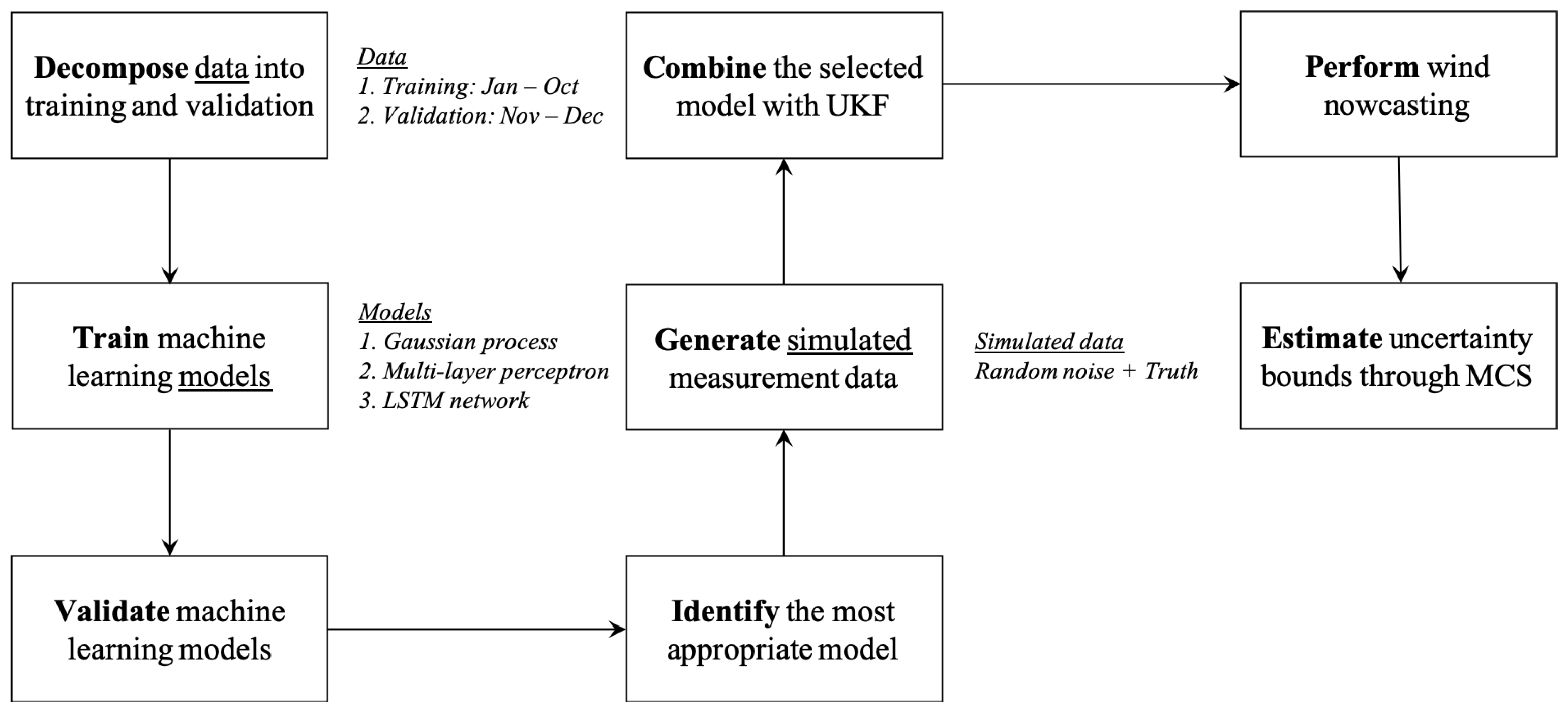
Figure 1. Overall flowchart of the proposed methodology.
Aerospace 08 00236 g001
Figure 2. Example visualization of the MERRA-2 winds at a specific time and altitude.
Aerospace 08 00236 g002
Figure 3. Decomposition of the MERRA-2 annual (2018) wind data into training (January–October) and validation (November–December) phases.
Aerospace 08 00236 g003
Figure 4. Diagram of the MLP structure used in this paper.
Aerospace 08 00236 g004
Figure 5. Performance evaluation of the machine learning prediction models to the validation phase datasets (2018 November–December).
Aerospace 08 00236 g005aAerospace 08 00236 g005b
Figure 6. Overview of the UKF-aided LSTM method framework.
Aerospace 08 00236 g006
Figure 7. Notional sketch of the MCS-based UQ process flowchart.
Aerospace 08 00236 g007
Figure 8. Performance comparison of wind nowcasting approaches (i.e., UKF-LSTM vs. LSTM only) to the test datasets (January 2019).
Aerospace 08 00236 g008
Table 1. DoE results for the hyper-parameters of the MLP model.
HyperparameterLower BoundUpper BoundFinal Choice
Number of hidden layers122
Number of hidden nodes1010050
Learning rate0.010.000010.0001
Regularization penalty parameter0.010.000010.001
Batch size1400200
Table 2. LSTM network structure used in this paper.
ParameterValue
Number of layers6
Number of nodes30
Number of epochs100
Learning rate0.001
Dropout rate (hidden layer)0.2
Table 3. Comparison of machine-learning-based time-series wind prediction models.
ModelEastward Wind Prediction
RMSE (m/s)MAE (m/s)R-Squared
LSTM3.91932.93540.9525
MLP6.74255.11570.8593
GP4.24143.10510.9433
ModelNorthward Wind Prediction
RMSE (m/s)MAE (m/s)R-Squared
LSTM4.44863.23350.9410
MLP4.99473.42740.9257
GP4.95383.49260.9269
Table 4. Comparison of the proposed approach (i.e., UKF-LSTM) with the LSTM-only approach.
ApproachEastward Wind Prediction
RMSE (m/s)MAE (m/s)R-Squared
UKF-LSTM3.22042.58280.9267
LSTM Only11.55248.91160.0567
ApproachNorthward Wind Prediction
RMSE (m/s)MAE (m/s)R-Squared
UKF-LSTM3.32052.67630.9767
LSTM Only22.441718.1376−0.0632
Publisher’s Note: MDPI stays neutral with regard to jurisdictional claims in published maps and institutional affiliations.