
Modeling and Control of a Modular Iron Bird

 ,
,  , ,
, ,  and
and 
Abstract
1. Introduction
2. The MIB Testing Facility
- the Data Acquisition and Control System (DACS). This is deployed on different hardware components, namely:
- –
- the Real-Time Process Controller (RTPC) implementing the so called Process Control Algorithms for the tracking of desired loads on the aerodynamic surfaces and the actuator unit under test reference positions;
- –
- the host PC implementing the User Interfaces (UI) for test preparation, on-line monitoring of the test variables, data archiving, post-processing functions and off-line visualization of the test results;
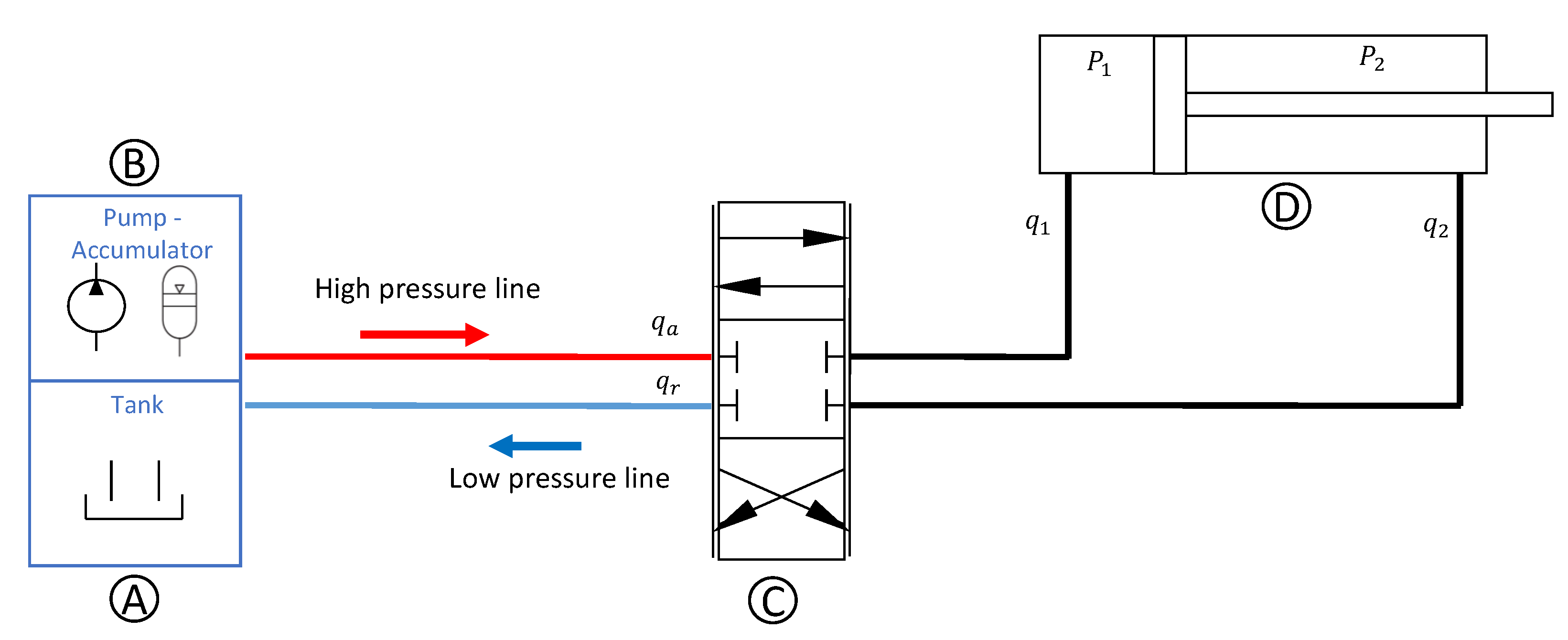
- a given number of Test Stands (TS) (see Figure 1), actually five, which are composed of:
- –
- a loading hydraulic actuator linked to a rigid mobile surface;
- –
- a set of pressure, position and load sensors, needed for control purposes and to acquire and archive test data;
- –
- the EMA Unit Under Testing (UUT) which is mechanically loaded by the hydraulic actuator;
- the Hydraulic Power Unit (HPU) to supply hydraulic pressure to the actuators on all the TSs;
- the Electrical Power Systems (EPSs).
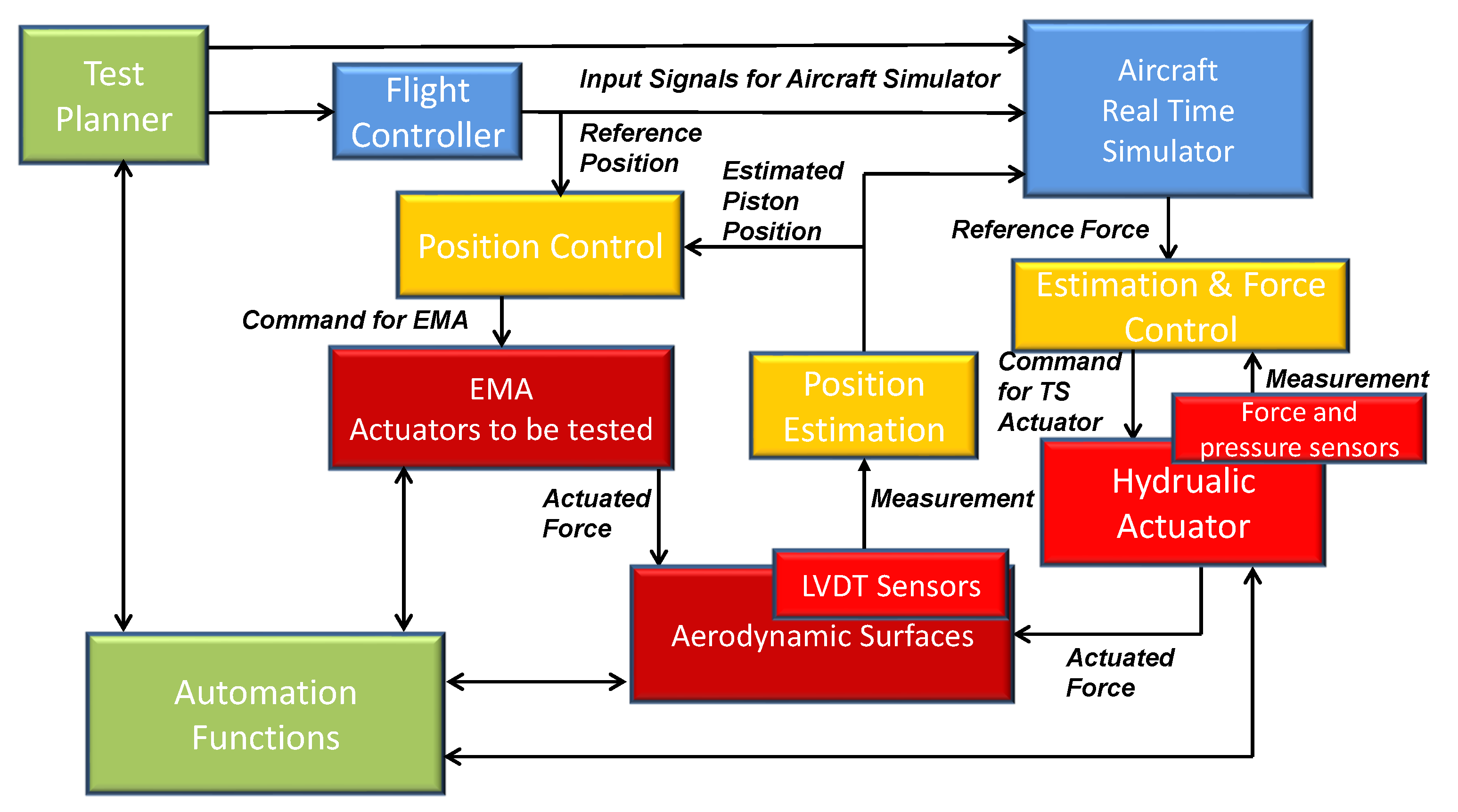
2.1. The Process and Automation Control System
- the test set up and automation functions (Green blocks),
- the real time simulator of the flight dynamics including flight controllers (Blue blocks),
- the actuators and sensor for the force control (Red blocks),
- the EMA actuator UUT (Dark Red block),
- the estimation of the surface position, the estimation of the force acting on the aerodynamic surface, and both the position and force controllers (Yellow blocks).
2.2. The Test Planner
- EMA Direct Control: the EMA is directly controlled, bypassing the Position Control;
- EMA Closed Loop Position Control: the position controller is activated to compute the EMA control signal.
- Hydraulic system Direct Control: the Force Controller is disabled in order to directly control the valve input signal. This test type can be useful in the first phases of the plant operation, in order to identify parameters of the hydraulic system dynamic model;
- Hydraulic system Closed Loop Control: the Force Controller is enabled and computes the servo-valve command on the basis of reference forces.
- Pre-programmed mode: the ARTS simply forwards waveforms designed through the TP GUI (both reference forces to the hydraulic system, and reference positions to the EMA controller).
- Self-consistent mode: the ARTS, on the basis of a reference manoeuvre defined by the TP, and the measured aerodynamic surface positions, calculates in real time the reference signals to the EMA position controllers and to the force controller.
3. Control Oriented Plant Mathematical Modeling
- -
- the HPU (a Rexroth Cytropack system) comprehensive of an accumulator and regulation system of the pressure inside the accumulator is modeled as a whole with a simple uncertain dynamics;
- -
- pipes dynamics are neglected. In fact, although they have been modeled, it has been verified in simulation that the dynamics are fast enough with respect to the characteristic times of interest, whereas their friction can be concentrated in the neighbouring elements;
- -
- wall deformation are neglected as their uncertain effect on closed loop control can be somehow evaluated with a larger uncertainties on the air trapped in the hydraulic fluid;
- -
- hard non-linearities as backlashes and dead zones and saturation are not taken into account in the controller design phase but simulated in the control performance evaluation.
EMA Actuator under Testing
4. Force Control Algorithm
- a set of uncertainties, defined in terms of variations with respect to nominal value of the following parameters:
- –
- Bulk modulus
- –
- air trapped volume ratio ,
- –
- Servo-valve time constant .
- –
- Discharge coefficient and servo-valve area product ,
- –
- EMA time constant .
A family of plant models, implementing the above uncertainties, is defined:(), where , , and u are the state vector, the controlled output (force on the aerodynamic surface) and control input (servo-valve command), respectively; - a set of operating scenarios to evaluate the robust performance of the controller over the models by means of the following cost function:with the output tracking error, being the force reference signal, the initial state at time , a finite time for the cost function evaluation, and w a suitable vector of weights;
- a parametric structure for the force controller:with . In our case, the vector p represents the gains of a PID control action to be optimized.
5. Numerical Result
- Scenarios without the Aircraft simulator:
- –
- force multi step (with increasing amplitude 100, 500 and 1000 N), constant pump pressure (15 MPa);
- –
- force multi step with constant pump pressure of the nominal 15 MPa);
- –
- force multi step with constant pump pressure of the nominal 15 MPa);
- –
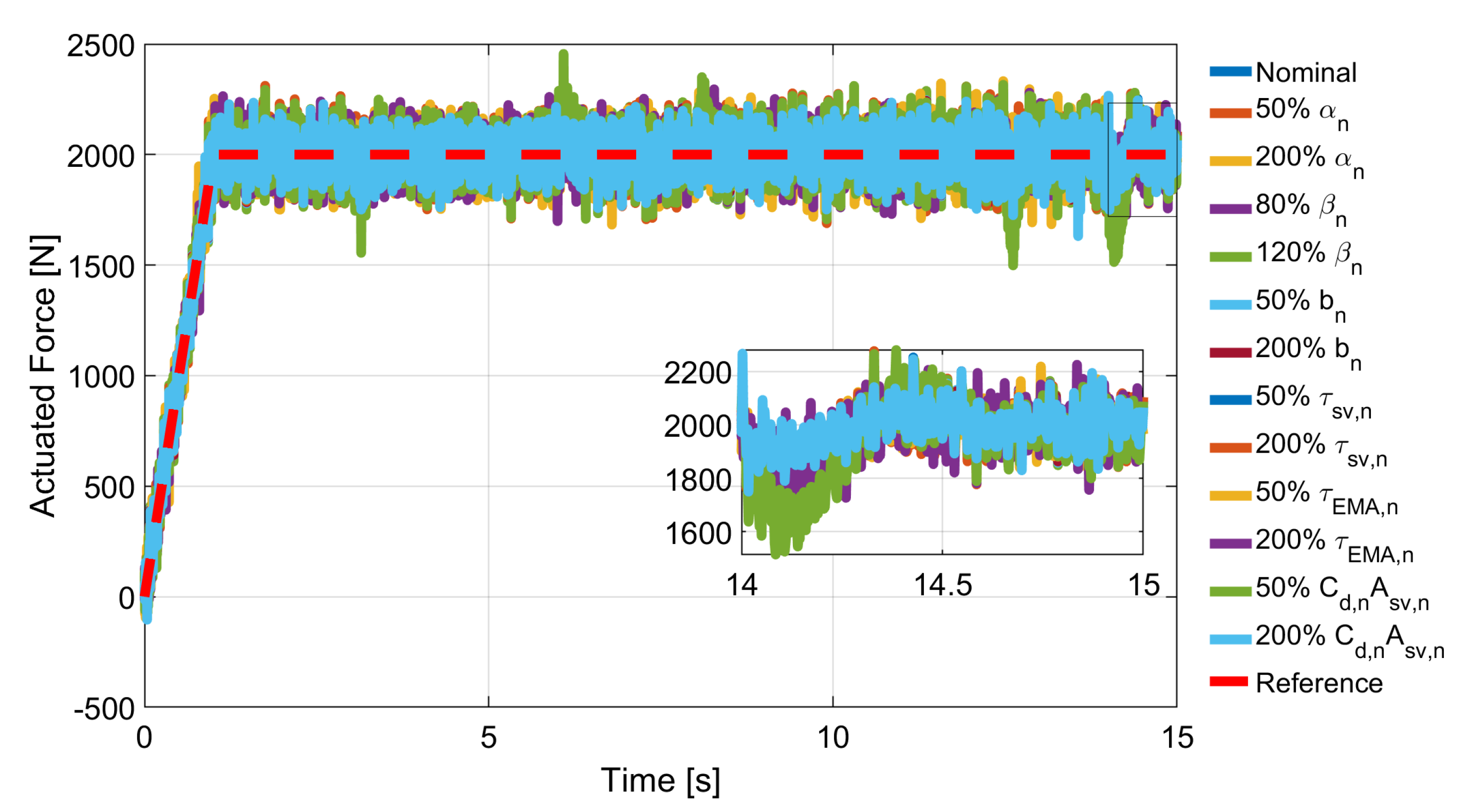
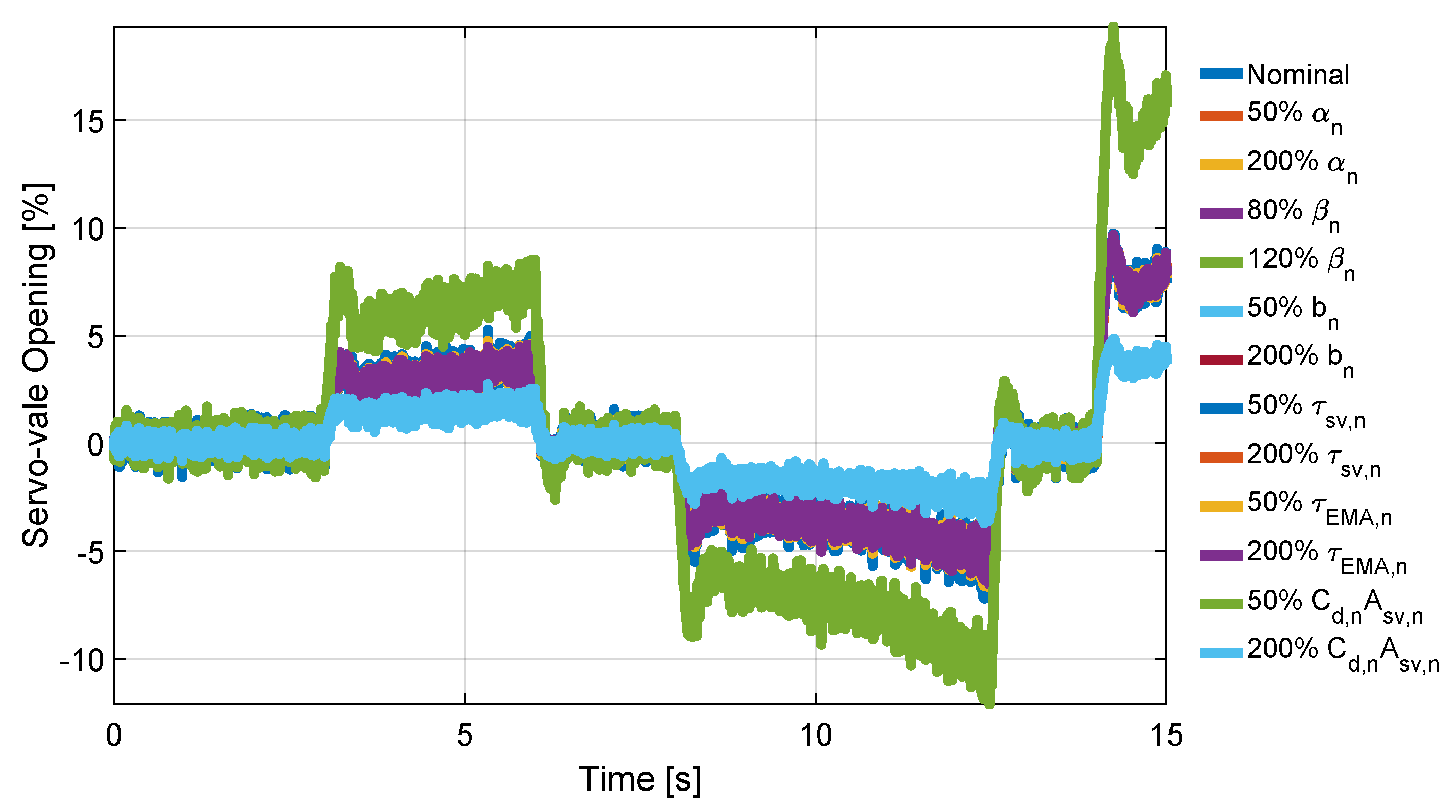
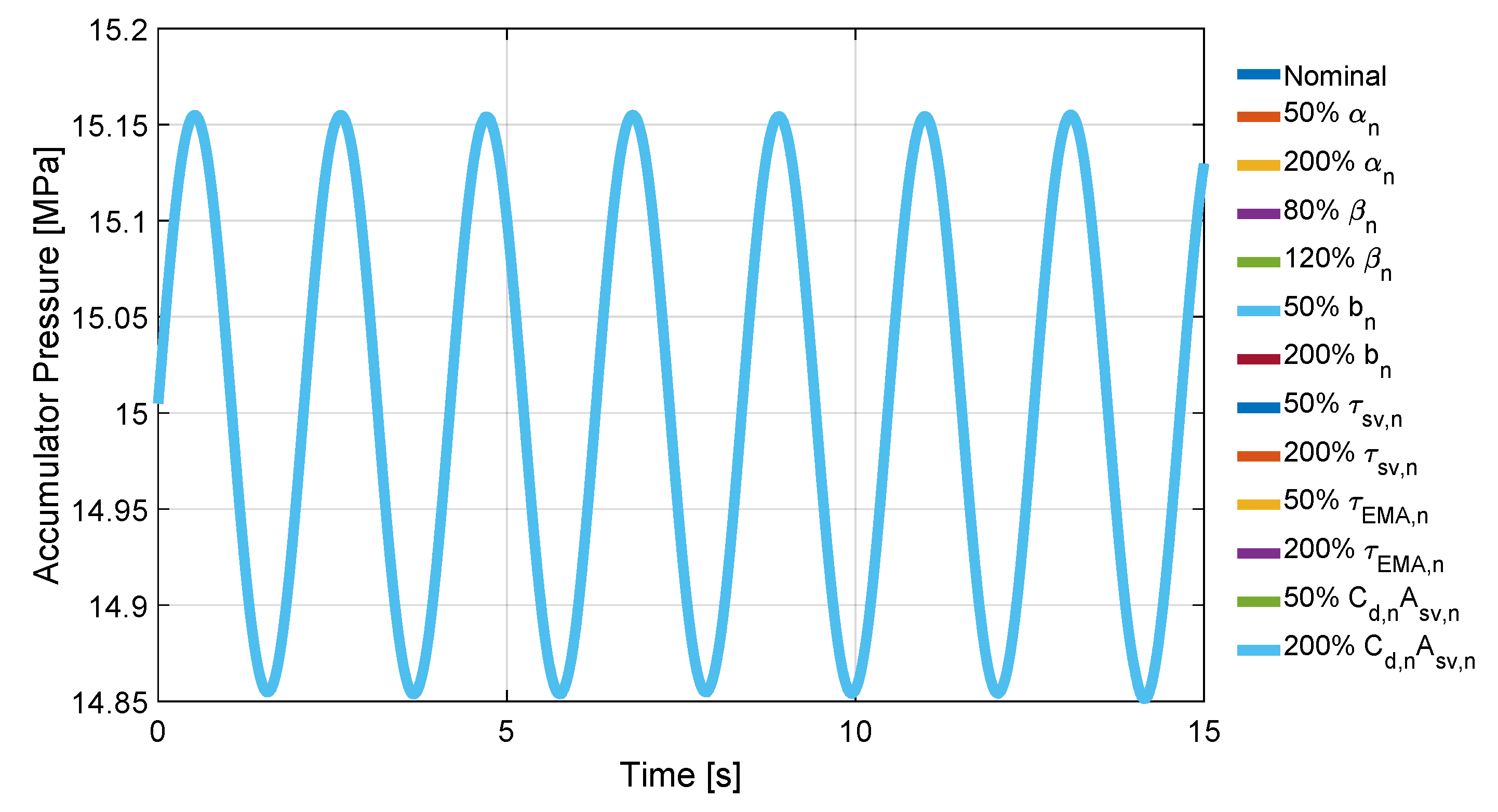
- force multi step with sinusoidal pump pressure (15 MPa+ 0.15 sin() MPa).
- Scenarios with the Aircraft simulator:
- –
- Aileron doublet (2.5 deg deflection for 9 s followed by −2.5 deg deflection for 9 s);
- –
- Aileron step (2.5 deg deflection).
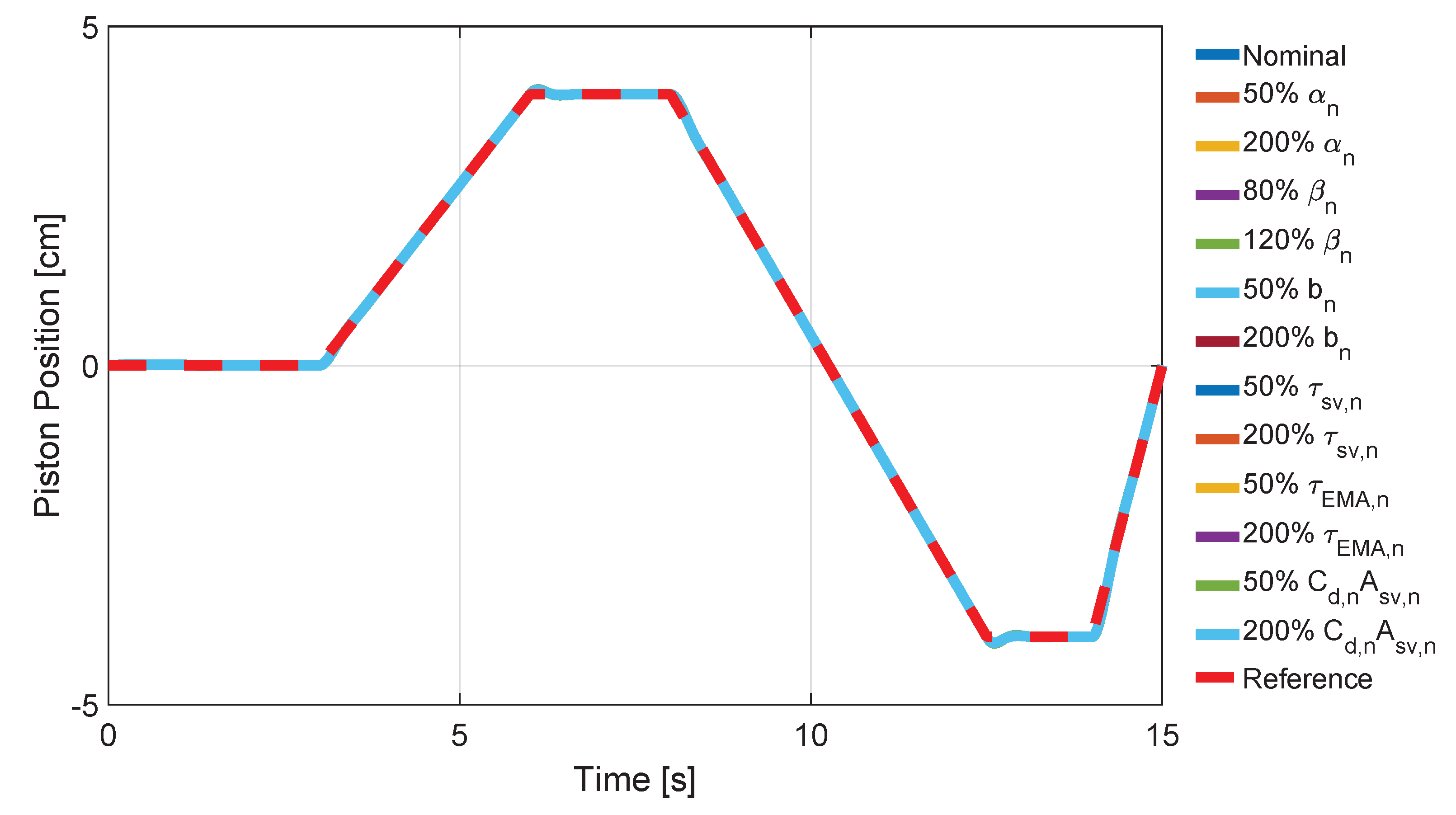
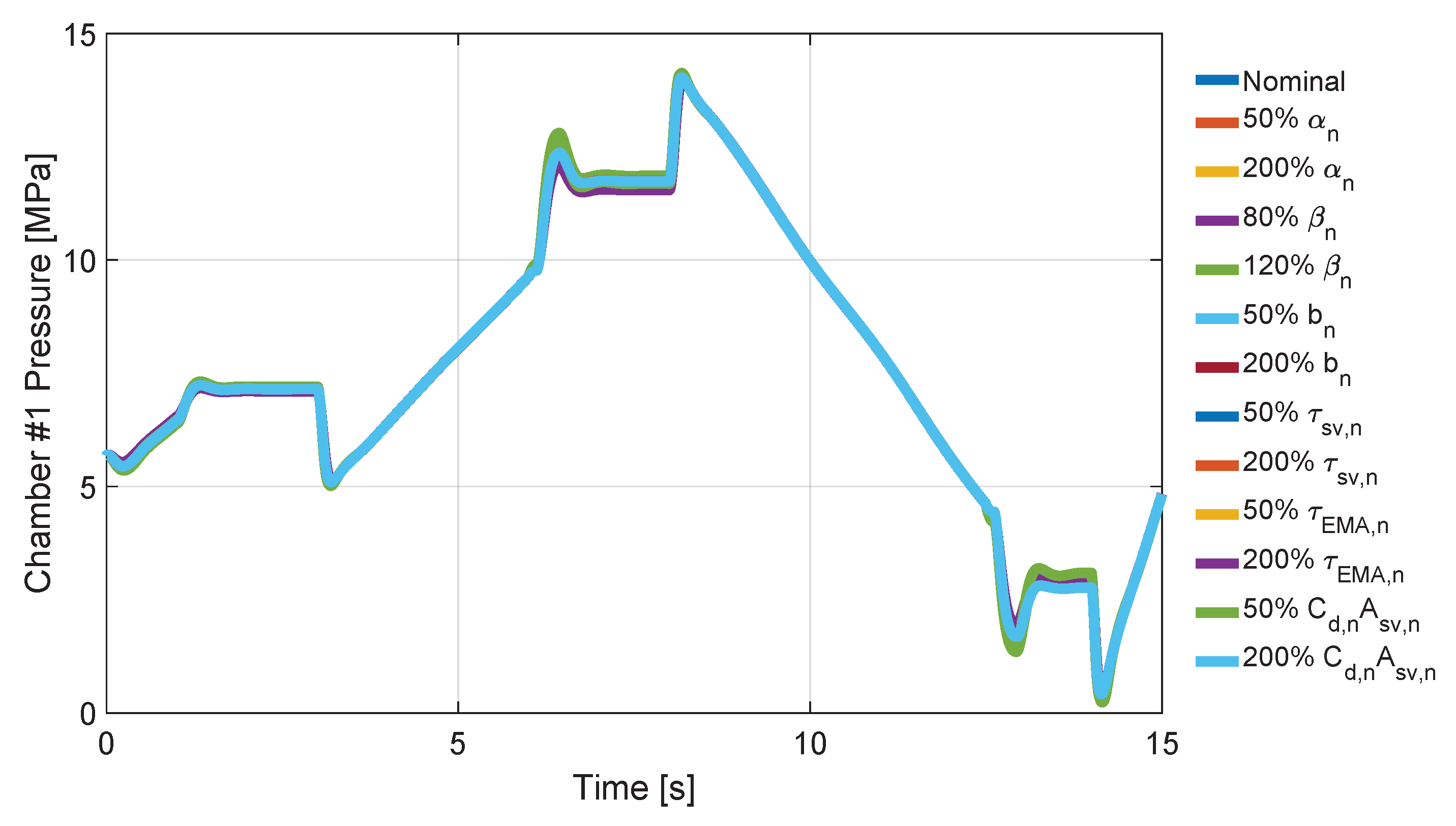
- of the nominal bulk modulus at atmospheric pressure;
- of the nominal air trapped volume ratio;
- of the servo-valve time constant;
- of the parameter;
- of EMA time constant.
Numerical Results with the Flight Simulator in the Loop
- without FCS:
- –
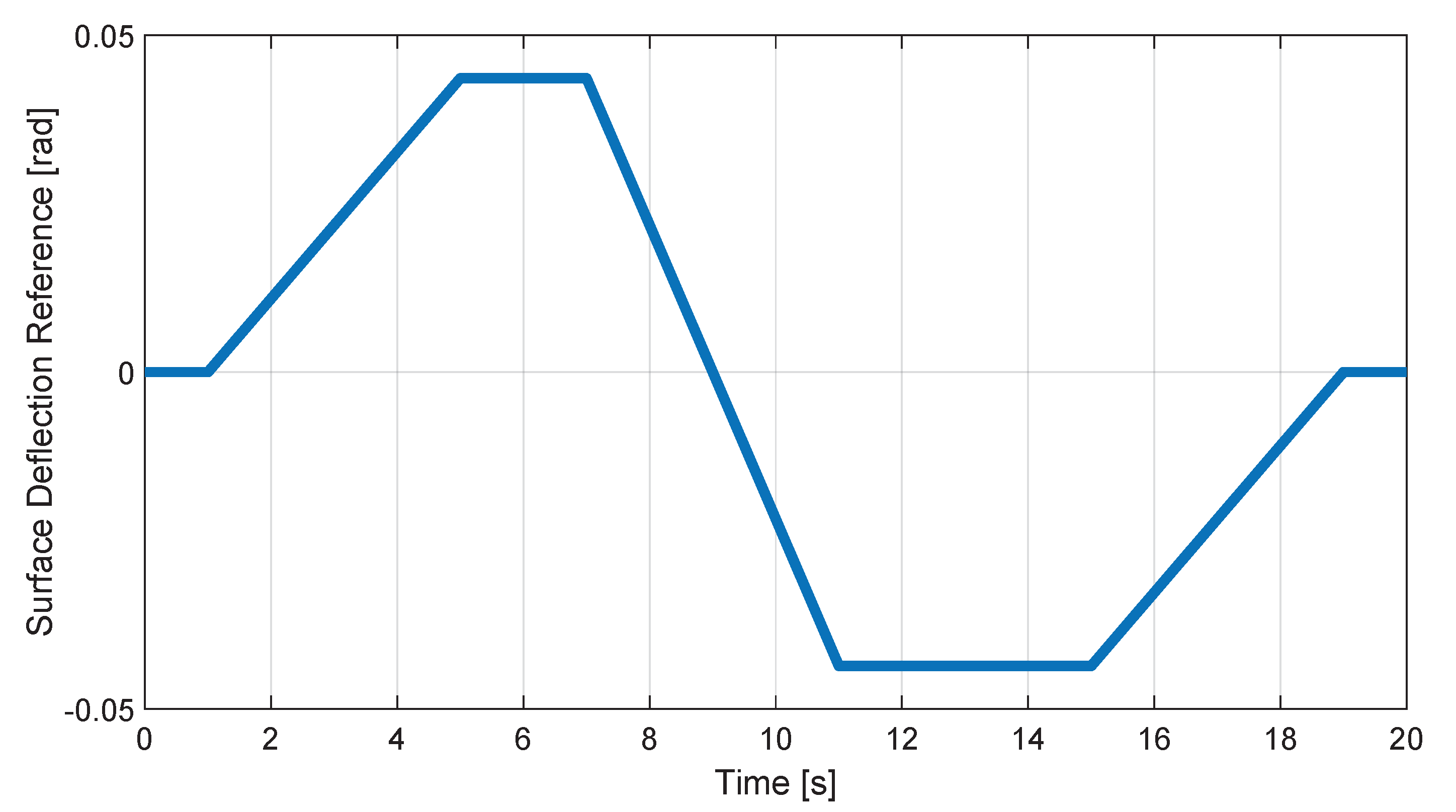
- a 0.044 rad step on ailerons deflection;
- –
- a ±0.044 rad doublet on ailerons deflection;
- with SAS active:
- –
- a 0.044 rad step on ailerons deflection;
- –
- a ±0.044 rad doublet on ailerons deflection;
- with CAS active:
- –
- an impulse (1.05 rad/s) on roll rate command;
- –
- a doublet (±1.05 rad/s) on roll rate command;
- with Autopilot active:
- –
- a step (0.088 rad) on the heading angle reference;
- –
- a ramp (0.26 rad/s) on heading angle reference;
6. Conclusions
Author Contributions
Funding
Institutional Review Board Statement
Informed Consent Statement
Data Availability Statement
Conflicts of Interest
References
- Prasad, M.; Gangadharan, K. Aileron endurance test rig design based on high fidelity mathematical modeling. CEAS Aeronaut. J. 2017, 8, 653–671. [Google Scholar] [CrossRef]
- Maré, J.C. Aerospace Actuators 2: Signal-By-Wire and Power-By-Wire; John Wiley & Sons: Hoboken, NJ, USA, 2017. [Google Scholar]
- Wheeler, P.; Bozhko, S. The More Electric Aircraft: Technology and challenges. IEEE Electrif. Mag. 2014, 2, 6–12. [Google Scholar] [CrossRef]
- Jean-Charles, M.; Jian, F. Review on signal-by-wire and power-by-wire actuation for more electric aircraft. Chin. J. Aeronaut. 2017, 30, 857–870. [Google Scholar]
- Wilcox, D.C. Formulation of the kw turbulence model revisited. AIAA J. 2008, 46, 2823–2838. [Google Scholar] [CrossRef]
- Rubertus, D.P.; Hunter, L.D. Electromechanical actuation technology for the all-electric aircraft. IEEE Trans. Aerosp. Electr. Syst. 1984, AES-20, 243–249. [Google Scholar] [CrossRef]
- Qiao, G.; Liu, G.; Shi, Z.; Wang, Y.; Ma, S.; Lim, T.C. A review of electromechanical actuators for More/All Electric aircraft systems. Proc. Inst. Mech. Eng. Part C J. Mech. Eng. Sci. 2018, 232, 4128–4151. [Google Scholar] [CrossRef]
- Brière, D.; Traverse, P. AIRBUS A320/A330/A340 electrical flight controls-A family of fault-tolerant systems. In Proceedings of the FTCS-23 The Twenty-Third International Symposium on Fault-Tolerant Computing, Toulouse, France, 22–24 June 1993; pp. 616–623. [Google Scholar]
- Hwang, S.; Choi, S. Ironbird ground test for tilt rotor unmanned aerial vehicle. Int. J. Aeronaut. Space Sci. 2010, 11, 313–318. [Google Scholar] [CrossRef]
- Spangenberg, H.; Vechtel, D. Failure detection, identification and reconfiguration: Applications for a modular iron bird. In Proceedings of the AIAA Modeling and Simulation Technologies Conference and Exhibit, Hilton Head, SC, USA, 20–23 August 2007; p. 6466. [Google Scholar]
- De Martin, A.; Jacazio, G.; Sorli, M. Design of a PHM system for electro-mechanical flight controls: A roadmap from preliminary analyses to iron-bird validation. In Proceedings of the MATEC Web of Conferences, EDP Sciences, Sibiu, Romania, 5–7 June 2019; Volume 304, p. 04018. [Google Scholar]
- Topczewski, S.; Narkiewicz, J.; Bibik, P. Helicopter Control During Landing on a Moving Confined Platform. IEEE Access 2020, 8, 107315–107325. [Google Scholar] [CrossRef]
- Wang, C.; Jiao, Z.; Quan, L. Adaptive velocity synchronization compound control of electro-hydraulic load simulator. Aerosp. Sci. Technol. 2015, 42, 309–321. [Google Scholar] [CrossRef]
- Wang, C.; Jiao, Z.; Quan, L. Nonlinear robust dual-loop control for electro-hydraulic load simulator. ISA Trans. 2015, 59, 280–289. [Google Scholar] [CrossRef]
- Karpenko, M.; Sepehri, N. Electrohydraulic force control design of a hardware-in-the-loop load emulator using a nonlinear QFT technique. Control Eng. Pract. 2012, 20, 598–609. [Google Scholar] [CrossRef]
- Nam, Y. Dynamic Characteristic Analysis and Force Loop Design for the Aerodynamic Load Simulator. KSME Int. J. 2000, 14, 1358–1364. [Google Scholar] [CrossRef]
- Yao, B.; Chiu, G.T.; Reedy, J.T. Nonlinear adaptive robust control of one-dof electro-hydraulic servo systems. In ASME International Mechanical Engineering Congress and Exposition (IMECE’97); FPST: Fallon, NV, USA, 1997; Volume 4, pp. 191–197. [Google Scholar]
- Yao, B.; Bu, F.; Chiu, G.T. Non-linear adaptive robust control of electro-hydraulic systems driven by double-rod actuators. Int. J. Control 2001, 74, 761–775. [Google Scholar] [CrossRef]
- Ullah, N.; Wang, S.; Aslam, J. Adative robust control of electrical load simulator based on fuzzy logic compensation. In Proceedings of the 2011 International Conference on Fluid Power and Mechatronics, Beijing, China, 17–20 August 2011; pp. 861–867. [Google Scholar]
- Wang, C.; Jiao, Z.; Wu, S.; Shang, Y. A practical nonlinear robust control approach of electro-hydraulic load simulator. Chin. J. Aeronaut. 2014, 27, 735–744. [Google Scholar] [CrossRef]
- Kim, W.; Shin, D.; Won, D.; Chung, C.C. Disturbance-observer-based position tracking controller in the presence of biased sinusoidal disturbance for electrohydraulic actuators. IEEE Trans. Control Syst. Technol. 2013, 21, 2290–2298. [Google Scholar] [CrossRef]
- Shang, Y.; Liu, X.; Jiao, Z.; Wu, S. An integrated load sensing valve-controlled actuator based on power-by-wire for aircraft structural test. Aerosp. Sci. Technol. 2018, 77, 117–128. [Google Scholar] [CrossRef]
- Wang, L.; Mare, J.C. A force equalization controller for active/active redundant actuation system involving servo-hydraulic and electro-mechanical technologies. Proc. Inst. Mech. Eng. Part G J. Aerosp. Eng. 2014, 228, 1768–1787. [Google Scholar] [CrossRef]
- Manring, N.D.; Fales, R.C. Hydraulic Control Systems; John Wiley & Sons: Hoboken, NJ, USA, 2019. [Google Scholar]
- Jelali, M.; Kroll, A. Hydraulic Servo-Systems: Modelling, Identification and Control; Springer Science & Business Media: Berlin, Germany, 2012. [Google Scholar]
- Ali, H.H.; Fales, R.C. A review of flow control methods. Int. J. Dyn. Control 2021, 1–8. [Google Scholar] [CrossRef]
- Weerasooriya, S.; El-Sharkawi, M.A. Identification and control of a DC motor using back-propagation neural networks. IEEE Trans. Energy Convers. 1991, 6, 663–669. [Google Scholar] [CrossRef]
- Saab, S.S.; Kaed-Bey, R.A. Parameter identification of a DC motor: An experimental approach. In Proceedings of the ICECS 2001 8th IEEE International Conference on Electronics, Circuits and Systems (Cat. No. 01EX483), Malta, Malta, 2–5 September 2001; Volume 2, pp. 981–984. [Google Scholar] [CrossRef]
- Rubaai, A.; Kotaru, R. Online identification and control of a DC motor using learning adaptation of neural networks. IEEE Trans. Ind. Appl. 2000, 36, 935–942. [Google Scholar] [CrossRef]
- Yassin, I.M.; Taib, M.N.; Rahim, N.A.; Salleh, M.K.M.; Abidin, H.Z. Particle Swarm Optimization for NARX structure selection—Application on DC motor model. In Proceedings of the 2010 IEEE Symposium on Industrial Electronics and Applications (ISIEA), Penang, Malaysia, 3–5 October 2010; pp. 456–462. [Google Scholar] [CrossRef]
- Mare, J.C. Dynamic loading systems for ground testing of high speed aerospace actuators. Int. J. Aircr. Eng. Aerosp. Technol. 2006, 78, 275–282. [Google Scholar] [CrossRef]
- Jiao, Z.X.; Gao, J.X.; Qing, H.; Wang, S.P. The velocity synchronizing control on the electro-hydraulic load simulator. Chin. J. Aeronaut. 2004, 17, 39–46. [Google Scholar] [CrossRef]
- Niksefat, N.; Sepehri, N. Designing robust force control of hydraulic actuators despite system and environmental uncertainties. IEEE Control Syst. Mag. 2001, 21, 66–77. [Google Scholar]
- Di Rito, G.; Denti, E.; Galatolo, R. Robust force control in a hydraulic workbench for flight actuators. In Proceedings of the 2006 IEEE Conference on Computer Aided Control System Design, 2006 IEEE International Conference on Control Applications, 2006 IEEE International Symposium on Intelligent Control, Munich, Germany, 4–6 October 2006; pp. 807–813. [Google Scholar]
- Conrad, F.; Jensen, C. Design of hydraulic force control systems with state estimate feedback. IFAC Proc. Vol. 1987, 20, 307–312. [Google Scholar] [CrossRef]
- Bertucci, A.; Mornacchi, A.; Jacazio, G.; Sorli, M. A force control test rig for the dynamic characterization of helicopter primary flight control systems. Procedia Eng. 2015, 106, 71–82. [Google Scholar] [CrossRef][Green Version]
- Liu, G.; Daley, S. Optimal-tuning PID control for industrial systems. Control Eng. Pract. 2001, 9, 1185–1194. [Google Scholar] [CrossRef]
- Jacazio, G.; Balossini, G. Real-time loading actuator control for an advanced aerospace test rig. Proc. Inst. Mech. Eng. Part I J. Syst. Control Eng. 2007, 221, 199–210. [Google Scholar] [CrossRef]
- Pan, H.L.; Yan, J. Implement of electro-Hydraulic servo control of aero variable stroke plunger pump. In Advanced Materials Research; Trans Tech Publication: Stafa-Zurich, Switzerland, 2012; Volume 443, pp. 313–318. [Google Scholar]
- Zhu, Z.; Tang, Y.; Shen, G. Experimental investigation of a compound force tracking control strategy for electro-hydraulic hybrid testing system with suppression of vibration disturbances. Proc. Inst. Mech. Eng. Part C J. Mech. Eng. Sci. 2017, 231, 1033–1056. [Google Scholar] [CrossRef]
- Bu, F.; Yao, B. Nonlinear adaptive robust control of hydraulic actuators regulated by proportional directional control valves with deadband and nonlinear flow gains. In Proceedings of the 2000 American Control Conference (ACC), Chicago, IL, USA, 28–30 June 2000; Volume 6, pp. 4129–4133. [Google Scholar]
- Pratumsuwan, P.; Junchangpood, A. Force and position control in the electro-hydraulic system by using a MIMO fuzzy controller. In Proceedings of the 2013 IEEE 8th Conference on Industrial Electronics and Applications (ICIEA), Melbourne, VIC, Australia, 19–21 June 2013; pp. 1462–1467. [Google Scholar]
- Wang, X.; Wang, S.; Wang, X. Electrical load simulator based on velocity-loop compensation and improved fuzzy-PID. In Proceedings of the 2009 IEEE International Symposium on Industrial Electronics, Seoul, Korea, 5–8 July 2009; pp. 238–243. [Google Scholar]
- Li, X.; Zhu, Z.C.; Rui, G.C.; Cheng, D.; Shen, G.; Tang, Y. Force loading tracking control of an electro-hydraulic actuator based on a nonlinear adaptive fuzzy backstepping control scheme. Symmetry 2018, 10, 155. [Google Scholar] [CrossRef]
- Gizatullin, A.; Edge, K. Adaptive control for a multi-axis hydraulic test rig. Proc. Inst. Mech. Eng. Part I J. Syst. Control Eng. 2007, 221, 183–198. [Google Scholar] [CrossRef]
- Piché, R.; Pohjolainen, S.; Virvalo, T. Design of robust controllers for position servos using H-infinity theory. Proc. Inst. Mech. Eng. Part I J. Syst. Control Eng. 1991, 205, 299–306. [Google Scholar] [CrossRef]
- Yao, J.; Jiao, Z.; Shang, Y.; Huang, C. Adaptive nonlinear optimal compensation control for electro-hydraulic load simulator. Chin. J. Aeronaut. 2010, 23, 720–733. [Google Scholar]
- Kallu, K.D.; Wang, J.; Abbasi, S.J.; Lee, M.C. Estimated reaction force-based bilateral control between 3dof master and hydraulic slave manipulators for dismantlement. Electronics 2018, 7, 256. [Google Scholar] [CrossRef]
- Shi, C.; Wang, X.; Wang, S.; Wang, J.; Tomovic, M.M. Adaptive decoupling synchronous control of dissimilar redundant actuation system for large civil aircraft. Aerosp. Sci. Technol. 2015, 47, 114–124. [Google Scholar] [CrossRef]
- Borrelli, M.; D’Amato, E.; di Grazia, L.E.; Mattei, M.; Notaro, I. MPC load control for aircraft actuator testing. In Proceedings of the 2020 7th International Conference on Control, Decision and Information Technologies (CoDIT), Prague, Czech Republic, 29 June–2 July 2020; Volume 1, pp. 587–592. [Google Scholar] [CrossRef]
- Drabble, D.; Ponnapalli, P.V.S.; Thomson, M.G.A. Optimisation of PID Controllers—Optimal Fitness Functions. In Developments in Soft Computing; John, R., Birkenhead, R., Eds.; Physica-Verlag HD: Heidelberg, Germany, 2001; pp. 183–190. [Google Scholar]
- Tran, H.K.; Son, H.H.; Duc, P.V.; Trang, T.T.; Nguyen, H.N. Improved Genetic Algorithm Tuning Controller Design for Autonomous Hovercraft. Processes 2020, 8, 66. [Google Scholar] [CrossRef]


| Parameter | Value |
|---|---|
| Bulk nominal modulus at atmospheric pressure, [GPa] | 1.5 |
| Pressure controlled by pump in the accumulator, [MPa] | 15 |
| Density at atmospheric pressure, [kg/m] | 989 |
| Servo-valve discharge coefficient times Servo-valve hole area, [cm] | 0.03 |
| Servo-valve equivalent time constant, [s] | 0.01 |
| Chamber cross section, A [cm] | 8.00 |
| Dead volume of the chamber | |
| Piston mass, m [kg] | 1.00 |
| Fraction of trapped air at atmospheric pressure, | 0.01 |
| Performance Parameters | Force | Position |
|---|---|---|
| Max MQE | 200 N | 4.6 cm |
| Max Overshoot | ||
| Perturbed ST | 0.24 s | 0.72 s |
Publisher’s Note: MDPI stays neutral with regard to jurisdictional claims in published maps and institutional affiliations. |
© 2021 by the authors. Licensee MDPI, Basel, Switzerland. This article is an open access article distributed under the terms and conditions of the Creative Commons Attribution (CC BY) license (http://creativecommons.org/licenses/by/4.0/).
Share and Cite
Blasi, L.; Borrelli, M.; D’Amato, E.; di Grazia, L.E.; Mattei, M.; Notaro, I. Modeling and Control of a Modular Iron Bird. Aerospace 2021, 8, 39. https://doi.org/10.3390/aerospace8020039
Blasi L, Borrelli M, D’Amato E, di Grazia LE, Mattei M, Notaro I. Modeling and Control of a Modular Iron Bird. Aerospace. 2021; 8(2):39. https://doi.org/10.3390/aerospace8020039
Chicago/Turabian StyleBlasi, Luciano, Mauro Borrelli, Egidio D’Amato, Luigi Emanuel di Grazia, Massimiliano Mattei, and Immacolata Notaro. 2021. "Modeling and Control of a Modular Iron Bird" Aerospace 8, no. 2: 39. https://doi.org/10.3390/aerospace8020039
APA StyleBlasi, L., Borrelli, M., D’Amato, E., di Grazia, L. E., Mattei, M., & Notaro, I. (2021). Modeling and Control of a Modular Iron Bird. Aerospace, 8(2), 39. https://doi.org/10.3390/aerospace8020039