Abstract
Polymer-ceramic pressure-sensitive paint (PC-PSP) has been used for capturing unsteady pressure over aerodynamic surfaces. Spatial and temporal pressure information is calculated from the luminescent intensity produced by a PC-PSP, which provides a nonintrusive pressure measurement. Despite its benefits, the temperature dependency of PC-PSP makes extraction of quantitative pressure data challenging. The temperature dependency in terms of the static and dynamic characteristics of a ruthenium-based PC-PSP is studied herein. The impact of temperature dependency on PC-PSP characteristics is also discussed in the context of an unsteady pressure measurement.
1. Introduction
Polymer-ceramic pressure-sensitive paint (PC-PSP) has received significant attention as a method for unsteady pressure measurement over aerodynamic test articles [1,2,3]. Spatial and temporal pressure measurements using PC-PSP have been utilized for the comprehension of advanced flow fields [4,5]. The luminescent intensity from PSP is related to the partial pressure of oxygen in the air based on a photophysical process called oxygen quenching. A conventional PSP is comprised of luminescent molecules that are sensitive to pressure and an adhesive polymer that holds molecules in the PSP coating layer [6]. The luminescent intensity from a conventional PSP, in which oxygen-sensitive molecules are incorporated in the less gas-permeable polymer layer, responds to pressure change with a sub-second time response. The time response of a PSP can be improved to be in the order of microseconds by embedding porous particles into the coating layer [7]. The physical components and materials of which a PC-PSP is comprised determine its static and dynamic characteristics [8,9]. The selection of the oxygen-sensitive luminescent molecules and their solvent is the most crucial factor for the luminescent intensity and pressure sensitivity of the sensor [10,11]. The polymer-particle ratio (polymer content) and the layer thickness affect the dynamic characteristic of the PC-PSP [9,12].
Pressure and temperature fluctuate instantaneously in unsteady flow, which causes the luminescent intensity of a PSP to vary. The luminescent intensity is dependent on a temperature change due to thermal quenching. This temperature effect introduces additional uncertainty into the pressure measurement, which makes accurate measurement difficult. In order to compensate for the temperature effect, the surface temperature information is measured experimentally using temperature-sensitive paint (TSP) or an infrared (IR) camera [13,14,15]. Such methods capture the change in the luminescent intensity due to the temperature but do not account for the influence of the static/dynamic characteristics of PC-PSP, such as pressure sensitivity and time response. Ideally, the temperature effect is excluded from the measurement, but in principle, the complexities of a luminescent molecule make that impossible. It is therefore necessary to understand how changes in temperature impact unsteady pressure measurement using a PC-PSP. In this study, the influence of the static and dynamic characteristics is experimentally studied, and the overall temperature dependency of a PC-PSP as an unsteady pressure measurement is discussed.
2. Experimental Setup and Methods
2.1. Materials
A PC-PSP coating is a single-layer structure consisting of porous particles, adhesive polymer, and luminescent molecules (Figure 1). Porous particles and adhesive polymer were mixed in solution and sprayed over a test plate. The spray-coated test plate was then dipped in a separate luminophore solution. The recipe of the PC-PSP in this work followed that of previous studies [9,12]. The porous particle chosen, Silica gel (SiO2, Sigma-Aldrich, St. Louis MO, USA), was embedded into the PC-PSP coating layer. The porous particle has a microscale hollow structure, with a mean particle size between 2 and 25 μm. Room temperature vulcanizing (RTV) rubber (KE-41, Shin-Etsu Chemical Co. Ltd., Tokyo, Japan) was used as an adhesive polymer to attach the PC-PSP coating layer to the surface of the test plate. The two components were mixed together in a solution of dichloromethane, which was placed in an ultrasonicator for 20 min to separate aggregated particles. The polymer-to-particle ratio of the solution (polymer content) was 20% by weight. The mixed solution was sprayed to produce a layer 30 μm thick over 20 mm square aluminum plates. Spray-coated plates were placed in a vacuum oven to evaporate the application solvent. A 0.1 mM tris-(bathophenanthroline) ruthenium (II) chloride (GFS Chemicals) was dissolved in dichloromethane to produce the luminophore solution. Spray-coated plates were dipped into the luminophore solution for 20 min at room temperature. The dipped plates were then placed in a vacuum oven to evaporate excess solvent. Five test samples were prepared for an uncertainty analysis.

Figure 1.
Schematic of polymer-ceramic pressure-sensitive paint (PC-PSP).
2.2. Static Characterization
Figure 2 shows a schematic of the static characterization, whereby a spectrometer (F-7000, Hitachi High-Tech Corporation, Tokyo, Japan) was used to capture the spectral emission from the PC-PSP test plate under steady conditions. A test chamber was connected to both a pressure controller and a temperature controller. The pressure controller achieved the target pressure with 10 Pa accuracy, and the temperature controller had accuracy on the order of the second decimal degree. By controlling the pressure and temperature in the test chamber, pressure and temperature calibrations were obtained for the steady-state quantities of interest: luminescent intensity change, and pressure sensitivity. The excitation wavelength was 465 nm, and the excitation area covered the whole surface of the test plate. The spectrometer acquired the emission spectrum from 560 to 700 nm, including the 0.125% noise. The reference pressure and temperature were 100 kPa and 303 K, respectively. Dry air was pumped into the test chamber to minimize the effect of humidity on the PC-PSP [16]. The configuration of the optical setup was consistent across all measurements.
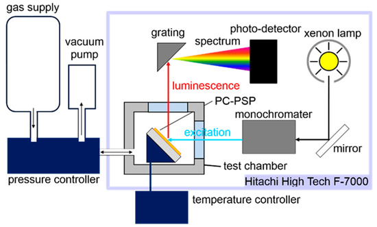
Figure 2.
Schematic of static characterization setup.
Theoretically, the luminescent intensity, I, is the product of the gain of the photo-detector in the spectrometer, G; the emission spectrum from the PC-PSP test plate, IPCPSP; the excitation intensity in the spectrometer, Iex; and a factor of due to the measurement setup, fset, as described in Equation (1) [17]:
Due to consistency in the measurement setup, G, Iex, and fset were constant for all tests so that IPCPSP was the only variable in the static characterization. During the pressure calibration, pressure, P, in the test chamber was varied from 5 to 120 kPa at the controllable reference temperature, Tref. The luminescent intensity ratio of the PC-PSP, I(Pref,Tref)/I(P,Tref) is described by the Stern–Volmer relationship in Equation (2) [1]:
where the subscript, ref, represents the reference conditions. A and B are calibration constants, which are functions of temperature. Because of the adsorption of oxygen molecules onto the porous layer, the intensity ratio of the PC-PSP behaves nonlinearly with changes in pressure [18]. Instead of a linear relationship, a second-order polynomial relationship is applied, as follows:
where AP, BP, and CP are calibration constants for the second-order polynomial fit. During actual unsteady pressure measurements, however, there can be a substantial difference in the reference temperature and the temperature during pressure measurements. In such an uncontrolled case, the measurement temperature, T, in the test chamber is different from the reference temperature, Tref,unc. In this case, the equation for the reference intensity, I(Pref,Tref,unc) is different from the luminescent intensity, I(Pref,Tref), described in Equation (4) due to the temperature difference between the reference and measurement temperatures:
where, AP,unc, BP,unc, and CP,unc are calibration constants under the uncontrolled reference temperature, Tref,unc. From Equation (3), the pressure sensitivity, σ, is defined as a slope of the luminescent intensity ratio:
In a similar manner as in the above case, but where the measurement temperature is different from the reference conditions, the pressure sensitivity from the Equation (4) is defined as
Due to thermal quenching, the luminescent intensity of the PC-PSP, I, is dependent on the temperature. The normalized luminescent intensity, I(T)/I(Tref), can be described with empirically-based polynomial functions. The first-order polynomial fit is
where, A and B are calibration constants under the first-order polynomial fit. The measurement temperature, T, in the test chamber was controlled from 273 to 333 K in 10 K steps to obtain the functional relationship between the normalized luminescent intensity and the temperature ratio during calibration. The reference pressure in the chamber was maintained at 100 kPa. A second-order polynomial fit can also be used to increase the number of terms to fit the calibration data [11,19]:
where, AT, BT, and CT are calibration constants for the second-order polynomial fit. If the measurement temperature, T, is the same as the reference temperature, Tref, the normalized luminescent intensity ratio is unity.
In the same manner as with pressure sensitivity, the luminescent intensity change, δ, for the first-order polynomial fit was defined as the slope of the normalized intensity, I(T)/I(Tref), at the reference temperature.
The luminescent intensity change, δ, for the second-order polynomial fit is
2.3. Dynamic (Dynamic-State) Characterization
The dynamic characteristics of PC-PSP were analyzed by observing the time response of the PC-PSP to a step-change in pressure. Figure 3 shows a schematic of a shock tube, which was used to generate a step-change in pressure. The luminescent intensity response of the PC-PSP has an inherent time delay and cannot measure instantaneous pressure changes. That time delay is herein referred to as the dynamic characteristic of the PC-PSP. A diaphragm separates the shock tube into two sections: a driven section at a lower pressure, and a driver section at a higher pressure. The lengths of the driven and driver sections were 1600 mm and 600 mm, respectively, with a cross-sectional area of 30 square mm. The test facility was purged with dry air. The absolute pressure in the driven and driver sections was 3 kPa and 130 kPa, respectively. The measurement temperature inside the entire shock tube was maintained at atmospheric temperature. Once the appropriate pressure difference had been achieved, the diaphragm burst. A normal shock wave with Mach number 2.1 propagated toward the driven section. The PC-PSP test plates and a pressure transducer (XCQ-062-50A, Kulite Semiconductor Products, Inc., Leonia, NJ, USA) were placed on the endplate of the driven section. A Peltier device was embedded into the endplate to control the temperature of the test plates, which were maintained at the reference temperature for the dynamic characterization. For each dynamic calibration, the temperature of the test plate was held to the reference temperature, which was a value between 283 and 363K, by the Peltier device. Before starting the dynamic calibration, the Peltier device held the temperature of the device constant to ensure the equilibrium of the test plate. That device had accuracy of the order of the second decimal degree. Because the temperature after the incident shock wave increases due to compressible effects, the reference and measurement temperatures were different; the measurement temperature was higher than that of the reference temperature. A blue laser with a wavelength of 465 nm illuminated the test plate as an excitation light source. An optical window on the side wall allowed the excitation and luminescent intensity from the PC-PSP test plate to pass through. A photomultiplier tube (PMT) (H57730-04, Hamamatsu Photonics K.K., Shizuoka, Japan) obtained the luminescent intensity and converted the acquired luminescent intensity to a voltage output. A bandpass filter (620 ± 20 nm) was placed in front of the PMT so that only emission from the PC-PSP test plate was acquired. The time response of the PMT was in the order of nanoseconds. The time response of the PC-PSP was in the order of ten to one hundred microseconds [12,20]; the PMT had a significantly faster time response than the PC-PSP, which ensured accurate measurement of the acquired the luminescent intensity. The pressure in the driven section, Pdrive, was monitored by the pressure transducer. Once the generated normal shock wave impinged on the endplate, the PC-PSP and the pressure transducer experienced a sharp pressure increase, Preflect. A normal shock wave induces not only a sharp increase in pressure but also in temperature. This near-instantaneous pressure increase was converted to a normalized pressure to extract the time delay of the PC-PSP [20,21,22]:
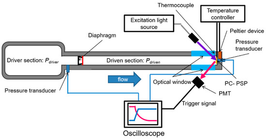
Figure 3.
Schematic of dynamic characterization setup.
Equation (4) is used to convert the obtained luminescent intensity, I, to pressure, P.
3. Results and Discussion
3.1. Luminescent Intensity Change
Figure 4 shows a representative luminescent spectrum obtained from the PC-PSP test plate under the reference pressure and temperatures at 100 kPa and 303 K, respectively. The integrated range from 600 to 640 nm is shown by the grayed section, which was used to determine as the luminescent intensity, I(P, T), for the static characterization.
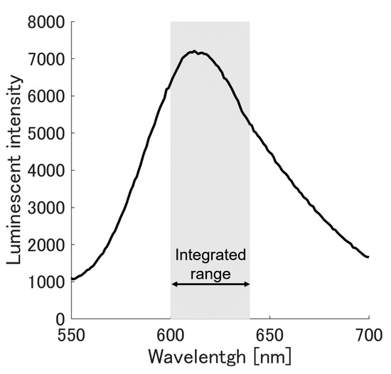
Figure 4.
Representative luminescent spectrum of the PC-PSP at Pref = 100 kPa, and Tref = 303 K.
From the temperature calibration plot shown in Figure 5, one can see a monotonic decrease in the normalized luminescent intensity, I(T)/I(Tref), with an increase in the temperature, T, from 273 to 333 K in 10 Kelvin steps. The reference luminescent intensity, I(Tref), was given at the reference temperature, Tref, of 303 K. Here, error bars on each calibration point are based on the standard deviation from the five calibrated test plates with 95% confidence interval. As described in Equation (8), a second-order polynomial fit adequately models the I(T)/I(Tref), shown as a red line. However, this second-order polynomial fit deviates from the data for temperatures higher than 313 K. The first-order polynomial fit, described in Equation (7), agreed with selected temperature ranges and was applied in the temperature calibration plot as dashed and dotted lines for 273–303 K and 303–333 K, respectively. The 95% prediction intervals were found for the three different polynomial fits. The first-order fit over the 303-333K temperature range had the tightest prediction band, which was only 4% of the normalized luminescent intensity. The second-order polynomial fit prediction band was 8% of the luminescent intensity or twice that of the best first-order fit.
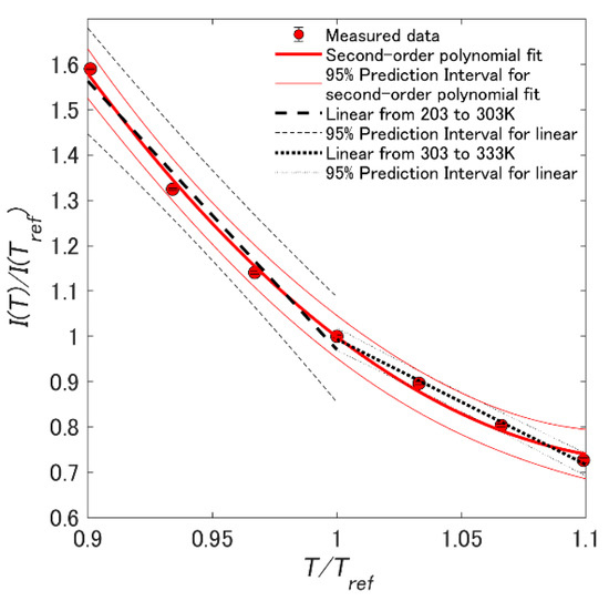
Figure 5.
Temperature calibration plot with normalized temperature T/Tref (Tref = 303 K).
Figure 6 shows the luminescent intensity change, δ, of the luminescent intensity, as a function of the reference temperature, Tref. The δ for each Tref was determined using Equations (9) and (10) for the linear and the second-order fits, respectively. The δ calculated using the second-order polynomial fit changed linearly with respect to Tref from −2.23% to −0.23% with a slope of 3.07% per Kelvin. This indicates that the rate of the luminescent intensity change due to the temperature varies by the reference temperature or by the measurement temperature. During an unsteady pressure measurement, there is a temperature distribution over a PC-PSP coated surface. If the second-order polynomial fit is used to describe δ, it is necessary to obtain a local measurement temperature to determine the distribution of δ over the PC-PSP surface. Instead of considering a δ distribution to understand the change in the luminescent intensity due to the temperature, Figure 6 suggests using a constant δ in a selected temperature range. As seen in Figure 5, a linear fit is acceptable in certain temperature ranges. The dashed and dotted lines calculated by the first-order polynomial fit within selected ranges were constant. The δ from the first-order polynomial fit in the temperature range 273–303 K was −1.71%, and δ in the temperature range 303–333 K decreased to −0.80%.
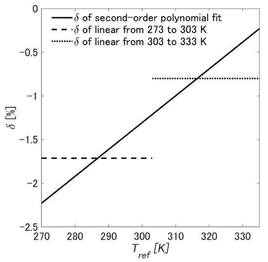
Figure 6.
Luminescent intensity change, δ, at each reference temperature, Tref.
3.2. Pressure Sensitivity
Figure 7 shows a representative pressure calibration plot between the luminescent intensity ratio I(Pref,Tref)/I(P,Tref) and the pressure ratio, P/Pref, under the controllable reference temperature, Tref. In the same manner as in the previous section, error bars were calculated for each calibration point based on the standard deviation from the five calibrated test plates with 95% confidence interval. Equation (3) was in agreement with the obtained I(Pref,Tref)/I(P,Tref) Both the reference and measurement temperature were the same as Tref. Figure 8 shows the temperature effect on the pressure sensitivity, σ, that was obtained by performing pressure calibrations over the temperature range 273 to 333 K at reference pressure, Pref. The σ for each reference temperature was determined using Equation (5) in the pressure calibration. The calculated σ ranged from 0.86 to 0.89%/kPa. The error bars based on 95% confidence interval of the calculated σ were obtained by repeating each pressure calibration five times. The effect of temperature on σ was within measurement uncertainty. If the reference temperature during an unsteady pressure measurement can be controlled, the value of σ can be considered constant.
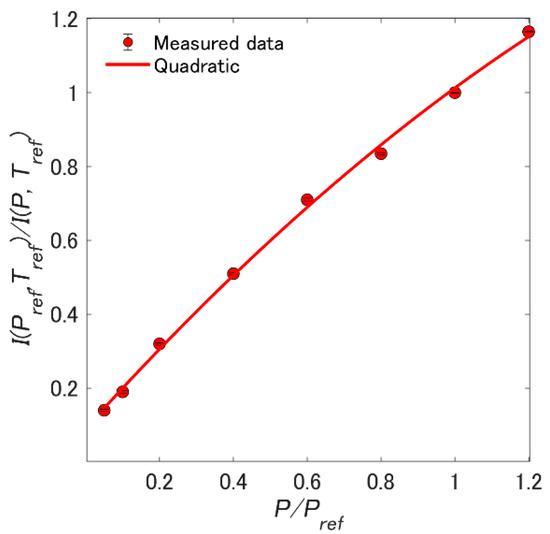
Figure 7.
Pressure calibration with the reference pressure Pref = 100 kPa and temperature Tref = 303 K.
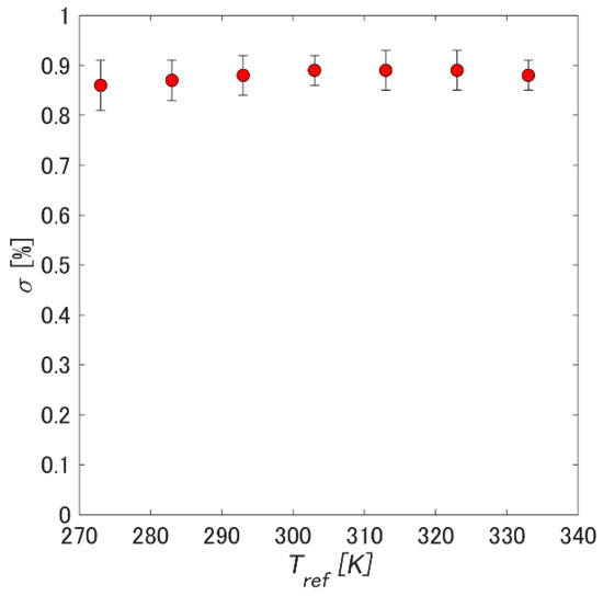
Figure 8.
Pressure sensitivity, σ, under varying the reference temperature, Tref.
Figure 9 shows the effect of measurement temperature on the pressure sensitivity, σ, for the uncontrolled case described by Equation (4). The value of σ was calculated with Equation (6) using pressure calibrations at various measurement temperatures, T, which were different from the reference temperature, Tref,unc. The value of Tref,unc was constant for the pressure calibrations. By varying T from 273 to 333 K with a constant value for Tref,unc, σ changed from 0.55 to 1.16%. This pressure calibration experimentally simulates conditions in which the reference temperature and the measurement temperature during the unsteady pressure measurement are not controlled to be the same. Applying a linear fir, the value of σ increases with slope of 1.06% per Kelvin. This slope indicates that the pressure sensitivity is dependent on the measurement temperature. This is distinct from the condition described in Figure 8, where the reference and measurement temperatures are the same or nearly the same and the pressure sensitivity can be considered as independent of the temperature.
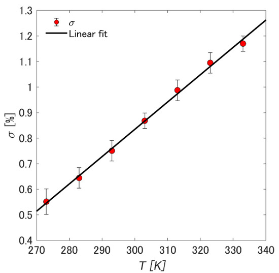
Figure 9.
Pressure sensitivity, σ, with varying the measurement temperature, T, under the uncontrollable reference temperature Tref,unc = 303 K.
3.3. Time Response
Figure 10 shows a representative step response of the PC-PSP test plate. The time response, τ, was defined as the time delay required for the PC-PSP to adjust to a step-change in pressure. The first-order system shown in Figure 10 is not appropriate to describe the response of the PC-PSP test plate. As shown in the figure, there are fast and slow components to the PC-PSPs response. Instead of applying the first-order system, the time response, τ, is defined as the time delay in reaching 90% of the normalized pressure, Pnorm. The PSP experienced pressure change as well as the temperature change by the compression due to a normal shock. The former was responded to by the oxygen quenching, and the latter was responded to by the thermal quenching. Figure 11 shows the value of τ under different reference temperatures, Tref. The value of τ fluctuated from 35 to 42 usec over the reference temperature range of 283 to 363 K. The error bars on the value of τ were obtained by repeating each dynamic characterization five times with 95% confidence interval. Within the given reference temperature range of 283–363 K characterized in this study, the temperature effect on the time response was less than 10.5%, which is within the measurement uncertainty of the response time. The temperature effect was calculated by the ratio between the mean response and the most deviated response. Because the temperature behind the reflected shock wave sharply increases, the values of Tref and T behind the reflected shock wave were not the same. Based on the compression due to a normal shock, the value of T behind the reflected shock wave rose to approximately 803 K when the temperature in the driven section was 298 K. This test experimentally simulated the conditions for which the reference and measurement temperatures are not controlled. The result indicates that the time response under the given temperature range characterized in this study is less affected by changes in temperature than the static characteristics discussed in the previous sections.
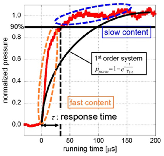
Figure 10.
Representative step response of the PC-PSP sample at reference temperature condition.
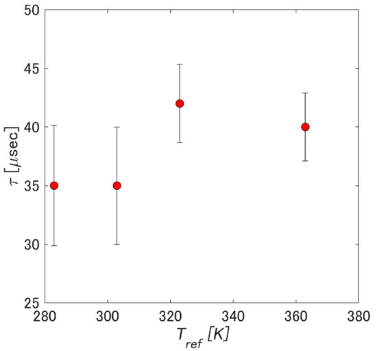
Figure 11.
Time response,τ, at each given reference temperature, Tref.
3.4. Discussion: Temperature Effect to Unsteady Pressure Measurement
Table 1 summarizes the temperature effect on the unsteady pressure measurement using PC-PSP. In using PC-PSP, it is necessary to acquire a reference image in addition to the measurement image. Under a controlled condition, both images can be acquired at the same temperature. In general, the reference temperature and the measurement temperatures are not the same. Herein, the former condition is called Case 1 and the latter Case 2. Both cases were experimentally simulated except for the time response of Case 1 due to the nature of the shock wave. If the reference and measurement temperatures can be controlled (Case 1), the static characteristics of the PC-PSP; the luminescent intensity change, δ; and pressure sensitivity, σ, can be considered constant with respect to temperature. If the reference and measurement temperatures are not the same, σ and δ show the temperature dependency. The σ increased by 1.06% per Kelvin, and δ increased by 3.07% per Kelvin, as temperature was increased. The dynamic characteristic of the time response had a minimal dependence on the temperature, which makes using PC-PSP for unsteady pressure measurement more favorable.

Table 1.
Temperature effect on the PC-PSP characteristics.
4. Conclusion
To show the effect of temperature on unsteady pressure measurements using PC-PSP, the temperature effect of a ruthenium-based PC-PSP was studied in both static and dynamic characterizations. In the static characterization, pressure and temperature calibrations on PC-PSP were conducted. Using a shock tube, the dynamic characteristic of the time response was studied as the function of temperature. Based on the two measurement conditions, where the reference temperature can be controlled or uncontrolled, the PC-PSP characteristics related to the temperature effects were investigated. For the case where the reference and measurement temperatures are controlled, two characteristics, luminescent intensity change due to temperature change and pressure sensitivity, are independent of the temperature. For the case where the reference and measurement temperatures are uncontrolled, luminescent intensity changes due to variations in temperature linearly and the pressure sensitivity increases with the reference temperature. It was confirmed that the time response of the PC-PSP has a minimal effect on the measurement temperature.
When conducting quantitative measurement with PC-PSP, the effect of temperature should be considered in the case where the reference and measurement temperatures cannot be controlled. The limited temperature change allows PSP users to assume the temperature dependency of the luminescent intensity change is constant. The time response of the PC-PSP can also be assumed to be independent of the temperature effect. By setting the appropriate measurement conditions, such as limiting allowed temperature changes and maintaining a controlled reference temperature, the pressure uncertainty related to the temperature effect can be minimized.
Author Contributions
T.H. and H.S. conceived and designed the experiments; T.H. performed the experiments and analyzed the data; T.H. wrote the original draft and H.S. review and edited the paper. All authors have read and agreed to the published version of the manuscript.
Funding
This research received no external funding.
Acknowledgments
The authors acknowledge the help of colleague Taku Tani in setting up the shock tube experiment and static calibration.
Conflicts of Interest
The authors declare no conflict of interest.
References
- Liu, T.S.; John, P.S. Pressure and Temperature Sensitive Paint; Springer: Berlin/Heidelberg, Germany, 2004; ISBN 3540222413. [Google Scholar]
- Currao, G.M.D.; Neely, A.J.; Kennell, C.M.; Gai, S.L.; Buttsworth, D.R. Hypersonic Fluid–Structure Interaction on a Cantilevered Plate with Shock Impingement. AIAA J. 2019, 57, 4819–4834. [Google Scholar] [CrossRef]
- Coschignano, A.; Babinsky, H. Boundary-Layer Development Downstream of Normal Shock in Transonic Intakes at Incidence. AIAA J. 2019, 57, 5241–5251. [Google Scholar] [CrossRef]
- Panda, J.; Roozeboom, N.H.; Ross, J.C. Wavenumber-Frequency Spectra on a Launch Vehicle Model Measured via Unsteady Pressure-Sensitive Paint. AIAA J. 2019, 57, 1–17. [Google Scholar] [CrossRef]
- Gößling, J.; Ahlefeldt, T.; Hilfer, M. Experimental validation of unsteady pressure-sensitive paint for acoustic applications. Exp. Therm. Fluid Sci. 2020, 112, 1–12. [Google Scholar] [CrossRef]
- Bell, J.H.; Schairer, E.T.; Hand, L.A.; Mehta, R.D. Surface Pressure Measurements Using Luminescent Coatings. Annu. Rev. Fluid Mech. 2001, 33, 155–206. [Google Scholar] [CrossRef]
- Gregory, J.W.; Asai, K.; Kameda, M.; Liu, T.; Sullivan, J.P. A review of pressure-sensitive paint for high-speed and unsteady aerodynamics. Proc. Inst. Mech. Eng. Part G J. Aerosp. Eng. 2008, 222, 249–290. [Google Scholar] [CrossRef]
- Quinn, M.K.; Yang, L.; Kontis, K. Pressure-sensitive paint: Effect of substrate. Sensors 2011, 11, 11649–11663. [Google Scholar] [CrossRef]
- Sakaue, H.; Kakisako, T.; Ishikawa, H. Characterization and optimization of polymer-ceramic pressure-sensitive paint by controlling polymer content. Sensors 2011, 11, 6967–6977. [Google Scholar] [CrossRef]
- Sakaue, H.; Hayashi, T.; Ishikawa, H. Luminophore application study of polymer-ceramic pressure-sensitive paint. Sensors 2013, 13, 7053–7064. [Google Scholar] [CrossRef]
- Egami, Y.; Konishi, S.; Sato, Y.; Matsuda, Y. Effects of solvents for luminophore on dynamic and static characteristics of sprayable polymer/ceramic pressure-sensitive paint. Sens. Actuators A Phys. 2019, 286, 188–194. [Google Scholar] [CrossRef]
- Hayashi, T.; Sakaue, H. Dynamic and steady characteristics of polymer-ceramic pressure-sensitive paint with variation in layer thickness. Sensors 2017, 17, 1125. [Google Scholar] [CrossRef]
- Peng, D.; Jiao, L.; Sun, Z.; Gu, Y.; Liu, Y. Simultaneous PSP and TSP measurements of transient flow in a long-duration hypersonic tunnel. Exp. Fluids 2016, 57, 1–16. [Google Scholar] [CrossRef]
- Yamashita, T.; Sugiura, H.; Nagai, H.; Asai, K.; Ishida, K. Pressure-sensitive paint measurement of the flow around a simplified car model. J. Vis. 2007, 10, 289–298. [Google Scholar] [CrossRef]
- Le Sant, Y.; Mérienne, M.C. Surface pressure measurements by using pressure-sensitive paints. Aerosp. Sci. Technol. 2005, 9, 285–299. [Google Scholar] [CrossRef]
- Kameda, M.; Yoshida, M.; Sekiya, T.; Nakakita, K. Humidity effects in the response of a porous pressure-sensitive paint. Sens. Actuators B Chem. 2015, 208, 399–405. [Google Scholar] [CrossRef]
- Liu, T.; Guille, M.; Sullivan, J.P. Accuracy of pressure-sensitive paint. AIAA J. 2001, 39, 103–112. [Google Scholar] [CrossRef]
- Sakaue, H. Luminophore application method of anodized aluminum pressure sensitive paint as a fast responding global pressure sensor. Rev. Sci. Instrum. 2005, 76, 1–6. [Google Scholar] [CrossRef]
- Egami, Y.; Sato, Y.; Konishi, S. Development of Sprayable Pressure-Sensitive Paint with a Response Time of Less Than 10 μs. AIAA J. 2019, 57, 2198–2203. [Google Scholar] [CrossRef]
- Pandey, A.; Gregory, J.W. Step response characteristics of polymer/ceramic pressure-sensitive paint. Sensors (Switzerland) 2015, 15, 22304–22324. [Google Scholar] [CrossRef]
- Carroll, B.; Abbitt, J.D.; Lukas, E.W. Step Response of Pressure-Sensitive Paints. AIAA J. 1996, 34, 521–526. [Google Scholar] [CrossRef]
- Sakaue, H.; Sullivan, J.P. Time response of anodized aluminum pressure-sensitive paint. AIAA J. 2012, 39, 1944–1949. [Google Scholar] [CrossRef]


© 2020 by the authors. Licensee MDPI, Basel, Switzerland. This article is an open access article distributed under the terms and conditions of the Creative Commons Attribution (CC BY) license (http://creativecommons.org/licenses/by/4.0/).