Abstract
This study used pressure-sensitive paint (PSP) and determined the surface pressure distributions for a compressible swept convex-corner flow. The freestream Mach numbers were 0.64 and 0.83. The convex-corner angle and swept angle were, respectively, 10–17° and 5–15°. Expansion and compression near the corner apex were clearly visualized. For the test case of shock-induced boundary layer separation, there were greater spanwise pressure gradient and curved shocks. The acquired PSP data agree with the experimental data measured using the Kulite pressure transducers for a subsonic expansion flow. For a transonic expansion flow, the discrepancy was significant. The assumption of a constant recovery factor is not valid in the separation region, and temperature correction for PSP measurements is required.
1. Introduction
Prandtl–Meyer expansion in supersonic and hypersonic flows is well known [1,2]. In subsonic and transonic flows, variable camber control using deflected control surfaces can be used to maximize the lift-to-drag ratio in different flight conditions [3]. A convex corner represents an idealized configuration for an upper control surface, and expansion and compression occur near the corner’s apex [4]. At higher freestream Mach numbers, M, and convex-corner angles, η, there is shock-induced boundary layer separation (SIBLS). Low-frequency shock motion (a few hundred Hertz) results in greater fluctuating loads. The peak value of surface pressure fluctuations reaches approximately 15% of the local mean surface pressure [5]. For a swept convex corner, Chung and Su [6] showed that an increase in the swept angle, λ, results in a delay in the transition from subsonic to transonic expansion flow and in SIBLS. The shock excursion phenomenon is alleviated, resulting in reduced peak pressure fluctuations. The value of the Strouhal number increases slightly with an increasing local peak Mach number, Mp, and approaches that of an unswept convex-corner flow. This corresponds to less shock excursion.
The pressure-sensitive paint (PSP) technique is an optical method and has been used extensively for global visualization of surface pressure patterns [7,8,9,10,11,12,13]. Luminescence molecules are dissolved in a chemical solvent and a polymer binder is added. The paint is then applied to the model surface. When the paint is illuminated by a selected excitation light source, the intensity of the emissions at longer wavelengths is inversely proportional to the amount of local surface pressure (Henry’s Law), which corresponds to law of partial pressure (Dalton’s Law). A change in temperature also affects the intensity due to thermal quenching [14]. The quantitative surface pressure distribution can be determined based on static calibration of the PSP sensors and the Stern–Volmer equation. Measurement uncertainty corresponds to cameras, light sources, test conditions and pressure/temperature sensitivity. Indeed, the experimental results obtained from the PSP technique showed good agreement with the results obtained using conventional discrete pressure taps.
A study by Chung and Su [6] only determined the longitudinal pressure distributions for a swept convex-corner flow using discrete pressure transducers. The spanwise pressure distribution was not addressed. This study used PSP, quantitatively visualizing global surface pressure patterns. The data using PSP sensors and pressure transducers were compared. Pressure variation in the spanwise direction on the characteristics of the flow-field was determined. The data are important for a deflected surface and variable camber control at transonic flow speeds. Temperature correction of the PSP measurements is also presented.
2. Experimental Setup
2.1. Transonic Wind Tunnel and Models
The experiments were conducted in a blowdown transonic wind tunnel at the Aerospace Science and Technology Research Center, National Cheng Kung University (ASTRC/NCKU). The facility includes two compressors, two air dryers (dew point ≈ −40 °C), a cooling water system, three storage tanks (volume = 180 m3), a hydraulic system and a tunnel, as shown in Figure 1. The square test section (600 mm2) with perforated top/bottom walls (6% porosity) and solid side walls was 1500 mm in length. A rotary perforated sleeve valve controlled the stagnation pressure, po. Two choke flaps downstream from the test section were used to monitor M under subsonic conditions. The test conditions were recorded using a PXI 6511 system (National Instruments, Austin, TX, USA).
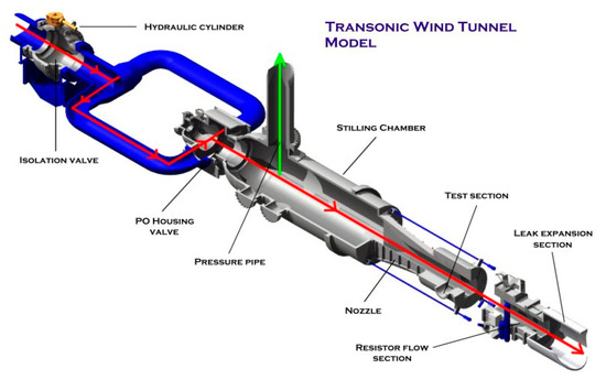
Figure 1.
Aerospace Science and Technology Research Center, National Cheng Kung University (ASTRC/NCKU) transonic wind tunnel.
A turbulent boundary layer was naturally developed along a flat plate (150 × 450 mm). Interchangeable plates (150 × 170 mm), as shown in Figure 2, with a swept convex corner (λ = 5°, 10° and 15°; η = 10°, 13° and 17°) were fabricated. The plates were supported by a single string mounted on the bottom wall of the tunnel. The values of po and the stagnation temperature, To, respectively, were 172 ± 0.5 kPa and room temperature, where M = 0.64 and 0.83 ± 0.01. The boundary-layer thickness, δ, 25 mm upstream of the convex corner was estimated to be approximately 7 mm [15]. Side plates were installed to prevent cross-flow.
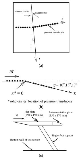
Figure 2.
Swept convex corner. (a) top view for swept convex corner; (b) side view for swept convex corner; (c) model support.
Conventional pressure measurements used the dynamic pressure transducers (Kulite XCS-093-25A, B screen). The transducers were flush-mounted and powered by a DC power supply (GW Instek PSS-3203, Taipei, Taiwan) of 10.0 V. Ectron amplifiers (753 A) were used to improve the signal-to-noise ratio. Each sample record had 131,072 data points with a 5-μs sampling rate. The experimental uncertainty was determined for the flat plate case. The value was 1.24% for the mean surface pressure coefficient, pw/p0,, where pw represents the mean surface pressure.
2.2. Pressure-Sensitive Paint
A polymer-ceramic PSP sensor was used in this study. Pt (II) meso-Tetra (pentafluorophenyl) porphine (PtTFPP), purchased from Frontier Scientific Co. (Logan, UT, USA), was chosen as the luminescence molecule and dissolved in ethanol (12 mg:12 mL). The absorption and emission spectra were determined at 392 nm and 650 nm, respectively. The lifetime was approximately 10 ms. Room-temperature-vulcanizing silicone (RTV 118; 1200 mg) was used as the polymer and mixed with porous particles (SiO2, 600 mg), with toluene (18 mL) as a porous binder. The PtTFPP solution was then mixed with the porous binder. The paint was applied to the surface for a plate with a swept convex corner using an air-spray gun. Pressure calibration (60–120 kPa) was conducted in a chamber with a pressure transducer (NOSHOK 100-30a-2-1-2-7, Berea, OH, USA). The paint was excited using two 2100-lumen white LED lamps (Revox SLG-55, Kanagawa, Japan) with a 550-nm short-pass optical filter. Luminescence images were acquired using a 14-bit scientific-grade Charge Coupled Device (CCD) camera (PCO Pixelfly, Regensburg, Germany; 1392 × 1040 pixels; 1 pixel ≈ 0.21 mm) with a 600-nm long-pass optical filter (20 frames/s). There were 50 images averaged. The Stern–Volmer equation was used to determine the calibration curve with the reference conditions of ambient pressure and 25 °C. The calibration curves for all test cases (η = 10°, 13° and 17°) are shown in Figure 3a for a pressure range of 0.34–1.43 atm. There was a linear relationship between the luminescence intensity ratio, Iref/I, and the pressure ratio, p/pref. The pressure sensitivity (PS) values calculated from the slope of Iref/I and p/pref were slightly different each other (=0.65–0.70%/kPa). The response time for PtTFPP using a shock tube was approximately 0.87 ms. Temperature sensitivity (TS) was determined using a customized temperature-controlled calibration chamber with a digital thermometer (YOTEC 947UD, Hsinchu, Taiwan). The temperature was varied from 5 °C to 34 °C. The value of Iref/I decreased with an increase in temperature, T, due to thermal quenching. The value of TS at the ambient pressure ranged from −1.9% to −2.1%/°C, as shown in Figure 3b. The Stern–Volmer equation for uniform temperature over the model surface can be expressed in the following equation:
where A(T) and B(T) are the Stern–Volmer coefficients for the case of T = Tref (=25 °C), and ΔT is the drop in model surface temperature.
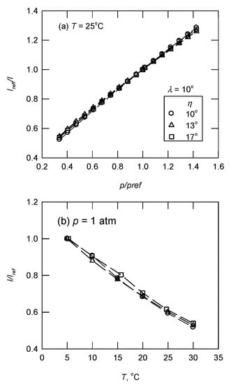
Figure 3.
Calibration curves for Pt (II) meso-Tetra (pentafluorophenyl) porphine (PtTFPP): (a) temperature (T) = 25 °C; (b) pressure (p) = 1 atm.
2.3. Data Reduction
The experimental uncertainty for PSP corresponded to detector noise, pressure resolution, model deformation, calibration and temperature effects [16]. It is known that errors due to model temperature changes are significant. In a blowdown wind tunnel, there is a drop in T; e.g., ≈3 °C during a typical blowdown duration of about 10 s for the present facility. This also results in a drop in the model’s surface temperature. The procedure for temperature correction is as follows:
- Correction of the pressure data due to the temperature effect can use the wind-off (post-run) images taken immediately after a tunnel shutdown as Iref [17].
- There may be a constant offset between pressure taps and the PSP. The most upstream pressure tap is used to account for the offset.
- The surface temperature can be modeled using the adiabatic wall temperature, Tr. with a recovery factor, r, of 0.896 for a turbulent boundary layer on a flat plate, in which [18]:
The error, σ, for all PSP data points with respect to Kulite sensors is calculated by:
3. Results and Discussion
3.1. Surface Pressure Pattern
For a swept convex-corner flow at M = 0.64, this was in the subsonic flow regime. Examples of global pressure distributions for η = 13° and 17° at λ of 10° are shown in Figure 4. The vertical color bar denotes pw/po, and the arrow corresponds to the incoming flow direction. There was upstream expansion, a strong favorable pressure gradient near the corner’s apex and downstream compression. The surface pressure pattern parallel to the swept corner appeared to be uniform or 2D in nature. The interaction region for η = 17° was greater than that for η = 13°; i.e., expanding both upstream and downstream. For a transonic expansion flow (M = 0.83), the flow expanded to supersonic speed and there was SIBLS [6]. The PSP images for λ = 10° are shown in Figure 5. For η = 10°, this corresponds to incipient flow separation. There was a greater downstream compression region than for M = 0.64. The surface pressure pattern also appeared to be 2D in nature. For η = 13° and 17°, a concave pressure pattern (axisymmetric pressure distributions) with respect to the centerline, but not near the side edges, was visible, particularly for η = 17°. This represents a spanwise pressure gradient. The images also show a greater adverse pressure gradient downstream from the corner. An increase in η resulted in an extension of the compression process, corresponding to the flow reattachment based on the oil flow visualization [6], shown as the solid line in Figure 5c.
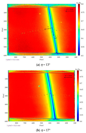
Figure 4.
Global surface pressure distribution for Mach number (M) = 0.64 and swept angle (λ) = 10°: (a) convex-corner angle (η) = 13°; (b) η = 17°.
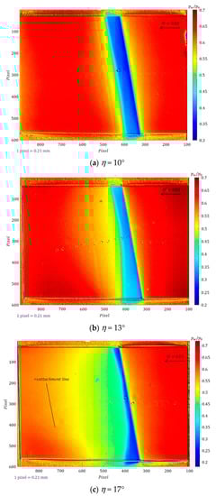
Figure 5.
Global surface pressure distribution for M = 0.83 and λ = 10°: (a) η = 10°; (b) η = 13°; (c) η = 17°.
3.2. Mean Surface Pressure Distribution
At M = 0.64, it is in the subsonic speed regime and there is no flow separation [6]. The pressure distributions in the longitudinal direction using the PSP (5 pixel × 5 pixel) and the Kulite sensors are shown in Figure 6, where the positive value of x* (=x/δ) denotes the non-dimensional distance perpendicular to the corner line. The origin of the horizontal axis is set at the corner’s apex. Expansion and compression near the corner apex are well determined by the PSP measurements. The difference between the two sensors ( is within ±3% for all test cases. For a transonic expansion flow (M = 0.83), the flow expands to supersonic speed (pw/po < 0.5283). The longitudinal pressure distributions at the centerline are shown in Figure 7. Upstream of the swept corner, the value of pw/po using the PSP sensor is greater than that using the Kulite sensors. The discrepancy between the two sensors is also clear downstream of the corner, particularly for the minimum value of pw/po, corresponding to Mp and for extensively SIBLS flow (η = 17°) [6]; i.e., and σ = 15.4% for λ = 15°. The most upstream pressure tap is used to account for the offset between the PSP and the Kulite sensors. Temperature correction based on the adiabatic wall temperature when a constant value of r is applied. In general, there was a significant reduction in the value of The corrected longitudinal pressure distributions for M = 0.83 and λ = 15° are presented in Figure 8. For η = 17°, σ is 6.3% and the peak value of is, respectively, 18.3% and 13.7% at x* = 0.43 and 1.29. However, there is temperature over-correction for x* ≥ 6.43; i.e., the average value of is −5.4% and 1.3% with/without temperature correction using a constant recovery factor.
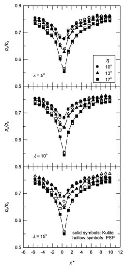
Figure 6.
Longitudinal pressure distribution at the centerline for M = 0.64.
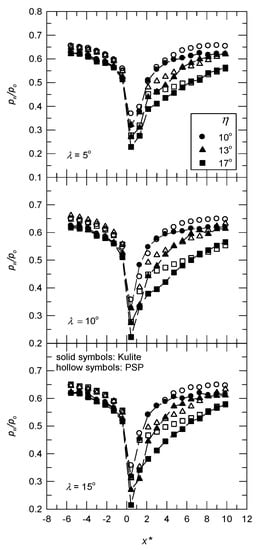
Figure 7.
Longitudinal pressure distribution at the centerline for M = 0.83.
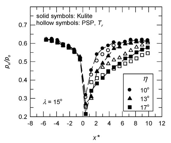
Figure 8.
Longitudinal pressure distribution at the centerline for M = 0.83 with a constant offset and recovery factor.
The spanwise pressure distribution downstream of the corner corresponds to the 3D nature of the flow, where Δpw/po (= is the variation in spanwise pressure with respect to the mean value, pw,avg. For M = 0.64 and λ = 10° (subsonic expansion flow), as shown in Figure 9, there are U-shaped distributions for η = 10° and 13° at x* = 0.43, 2.14 and 3.86. This is also true for η = 17° at x* = 2.14 and 3.86, but not for x* = 0.43 (an inverted U-shaped distribution), where the Mach number at the centerline, Mc, is 0.965. An increase in η results in a greater spanwise pressure gradient, , particularly for η = 17° at x* = 0.43 and y* (=y/δ) ≈ ±4. The spanwise pressure distributions for M = 0.83 and λ = 10° (transonic expansion flow) are shown in Figure 10. The incipient flow separation corresponds to η = 10°. U-shaped distributions are observed and the value of is greater than that for M = 0.64. For η = 13°, there are more uniform spanwise pressure distributions (or that are 2D in nature) at x* = 0.43 and 3.86. Near the separation location (x* = 2.14) [6], the amplitude of Δpw/po decreases from the left to the right. This reveals curved shocks, which are not parallel to the swept corner due to the spanwise pressure gradient. This is also true for η = 17° at x* = 2.14 and 3.86. The curved shock moves upstream and greater variation in the spanwise pressure distribution is observed at x* = 0.43.
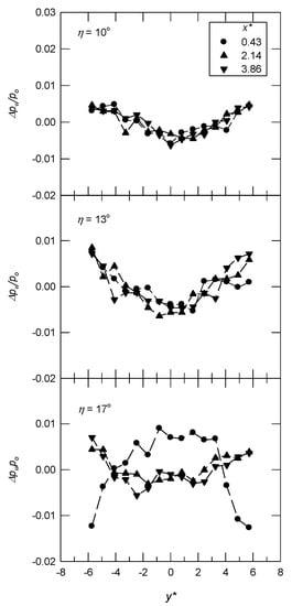
Figure 9.
Spanwise pressure distribution for M = 0.64 and λ = 10°.
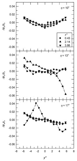
Figure 10.
Spanwise pressure distribution for M = 0.83 and λ = 10°.
3.3. Error Analysis
The value of σ, as shown in Equation (4), for the PSP data points along the longitudinal direction at the centerline with respect to the measurements using Kulite sensors is shown in Figure 11. In a subsonic expansion flow (M = 0.64), the value of σ is less than 2.7%. For M = 0.83 (a transonic expansion flow), there is a significant difference between the PSP and Kulite measurements, particularly for η = 17° and λ = 15° (σ = 15.4%). As shown in Figure 7, a constant offset is observed upstream of the swept corner, and the discrepancy downstream of the corner is also significant. The variation of σ with respect to Mp is shown in Figure 12a. Note that the value of Mp corresponds to the strength of the shock wave and SIBLS. For a specific λ value, there is greater discrepancy as Mp increases. Taking the offset and r into account, the maximum value of σ is 6.3% for η = 17° and λ = 15°, as shown in Figure 12b.
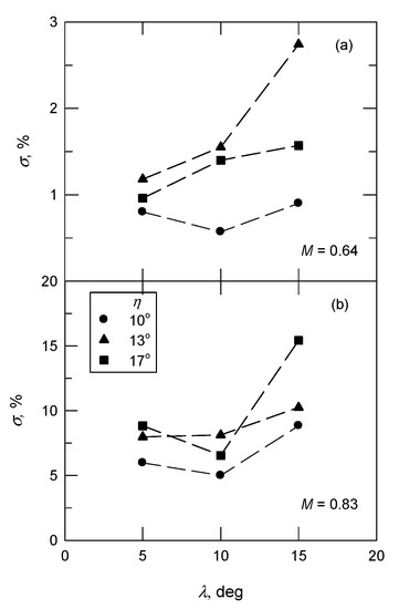
Figure 11.
The difference between longitudinal pressure distributions using pressure-sensitive paint (PSP) and Kulite sensors: (a) M = 0.64; (b) M = 0.83.
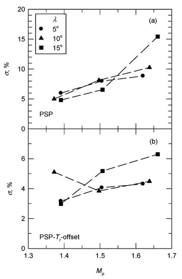
Figure 12.
The difference between longitudinal pressure distributions using PSP and Kulite sensors, corrected by a reference pressure tap and a recovery factor: (a) No temperature correction; (b) Temperature correction with a constant recover factor.
Pathak et al. [19] indicated that the constant value of r is questionable for a flow with SIBLS; i.e., the value of r is lower in a strong adverse pressure gradient; the opposite trend may be true in the presence of a favorable pressure gradient. An example (M = 0.83 and λ = 10°) of the difference between the PSP and Kulite measurements, Δ(pw/po)p-k (=, is shown in Figure 13. The locations of separation and reattachment, based on the oil flow visualization, are denoted as S and R, respectively. The offset ranged from 0.025 (η = 10°) to 0.038 (η = 13°). For η = 10° (incipient flow separation), the value of Δ(pw/po)p-k at x* = 1.28 was −0.042, implying an increase in the value of r. For the test cases of separated flow (η = 13° and 17°), the peak positive value of Δ(pw/po)p-k was observed near the separation location, following a decrease to a negative value near the reattachment location. At further downstream locations, the average value of Δ(pw/po)p-k was, respectively, 0.028 (x* ≥ 6.42) and 0.014 (x* ≥ 8.14) for η = 10° and 13°. This indicates that the assumption of the constant r fails in the separation bubble; i.e., there was an increase in the value of r from the separation to reattachment location. Therefore, for a reduction in the value of σ in a SIBLS flow, the surface temperature distribution, e.g., using temperature-sensitive paint in a separation bubble, is required.
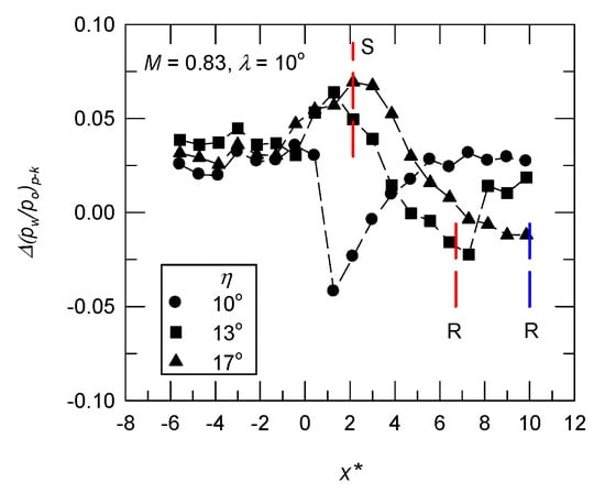
Figure 13.
Local flow structure of the difference between PSP and Kulite sensors for M = 0.83 and λ = 10°.
4. Conclusions
PSP measurements were conducted to visualize the global surface pressure patterns for a compressible swept convex-corner flow. The data were compared with pressure measurements using Kulite sensors. For a subsonic expansion flow without separation, the surface pressure pattern is 2D in nature and the PSP data agrees with the conventional pressure taps very well, in which the error is less than 2.7%. Curved shocks were observed near the separation location for a SIBLS flow due to the spanwise pressure gradient. Correction of the PSP results using a reference pressure tap and adiabatic wall temperature results reduced the deviation from the conventional pressure measurements; i.e., from 15.4% to 6.3% for η = 17° and λ = 15°. Assumption of a constant recovery factor is a quick way to compensate for the temperature effect for PSP measurements. It fails in the separation region, and surface temperature distribution using temperature-sensitive paint is required. In addition, active or passive flow control techniques can be used to reduce flow unsteadiness for a compressible swept convex-corner flow.
Author Contributions
Conceptualization, K.-M.C.; methodology, Y.-X.H.; formal analysis, K.-M.C.; resources, K.-M.C.; data curation, Y.-X.H.; writing—original draft preparation, Y.-X.H.; writing—review and editing, K.-M.C.; funding acquisition, K.-M.C. Both authors have read and agreed to the published version of the manuscript.
Funding
This research was funded by Ministry of Science and Technology, Taiwan, grant number MOST 107-2212-E-006-115-MY3.
Institutional Review Board Statement
Not applicable.
Informed Consent Statement
Not applicable.
Data Availability Statement
Not applicable.
Acknowledgments
The authors are grateful for the technical support of the ASTRC/NCKU technical staff.
Conflicts of Interest
The authors declare no conflict of interest.
Nomenclature
| I | luminescence intensity |
| Iref | luminescence intensity at atmospheric pressure |
| M | freestream Mach number |
| Mp | peak Mach number |
| p | surface pressure |
| pref | reference pressure for PSP measurements |
| p0 | stagnation pressure |
| pw | mean surface pressure using Kulite sensors |
| r | recovery factor |
| T | temperature |
| Tr | recovery temperature |
| ΔT | a drop in model surface temperature |
| x | longitudinal coordinate along the surface of the corner, mm |
| x* | normalized streamwise distance, x/δ |
| y | spanwise coordinate |
| y* | normalized spanwise distance, y/δ |
| δ | thickness of incoming boundary layer |
| η | convex-corner angle, degree |
| λ | swept angle, degree |
| σ | deviation between PSP and Kulite sensors |
References
- Lu, K.F.; Chung, K.M. Downstream influence scaling of turbulent flow past expansion corner. AIAA J. 1992, 30, 2976–2977. [Google Scholar] [CrossRef][Green Version]
- Chung, K.M. Interaction region of turbulent expansion-corner flows. AIAA J. 1998, 36, 1115–1116. [Google Scholar] [CrossRef]
- Szodruch, J.; Hilbig, R. Variable wing camber for transport aircraft. Prog. Aerosp. Sci. 1988, 25, 297–328. [Google Scholar] [CrossRef]
- Chung, K.M. Investigation on transonic convex-corner flows. J. Aircr. 2002, 39, 1014–1018. [Google Scholar] [CrossRef]
- Chung, K.M. Unsteadiness of transonic convex-corner Flows. Expt. Fluids 2004, 37, 917–922. [Google Scholar] [CrossRef]
- Chung, K.M.; Su, K.C. An experimental study on transonic swept convex-corner flows. Aerosp. Sci. Technol. 2019, 84, 565–569. [Google Scholar] [CrossRef]
- Peterson, J.I.; Fitzgerald, R.V. New technique of surface flow visualization based on oxygen quenching of fluorescence. Rev. Sci. Inst. 1980, 51, 670–671. [Google Scholar] [CrossRef]
- Liu, T.; Campbell, B.T.; Burns, S.P.; Sullivan, J.P. Temperature-and pressure-sensitive luminescent paints in aerodynamics. Appl. Mech. Rev. 1997, 50, 227–246. [Google Scholar] [CrossRef]
- Bell, J.H.; Schairer, E.T.; Hand, L.A.; Mehta, R.D. Surface pressure measurements using luminescent coatings. Annu. Rev. Fluid Mech. 2001, 33, 155–206. [Google Scholar] [CrossRef]
- Sakaue, H.; Kakisako, T.; Ishikawa, H. Characterization and optimization of polymer-ceramic pressure-sensitive paint by controlling polymer content. Sensors 2011, 11, 6967–6977. [Google Scholar] [CrossRef] [PubMed]
- Gregory, J.W.; Sakaue, H.; Liu, T.; Sullivan, J.P. Fast pressure-sensitive paint for flow and acoustic diagnostics. Annu. Rev. Fluid Mech. 2014, 46, 303–330. [Google Scholar] [CrossRef]
- Huang, C.Y.; Hu, Y.H.; Wan, S.A.; Nagai, H. Application of pressure-sensitive paint for the characterization of mixing with various gases in T-type micromixers. Int. J. Heat Mass Transf. 2020, 156, 119710. [Google Scholar] [CrossRef]
- Huang, C.Y.; Yeh, C.Y.; Lin, Y.F.; Chung, K.M. Global flow visualization of transonic cavity flow with various yaw angles. Proc. Inst. Mech. Eng. Part G J. Aerosp. Eng. 2021, in press. [Google Scholar] [CrossRef]
- Hayashi, T.; Sakaue, H. Temperature effects on polymer-ceramic pressure-sensitive paint as a luminescent pressure sensor. Aerospace 2020, 7, 80. [Google Scholar] [CrossRef]
- Bies, D.A. Flight and Wind Tunnel Measurements of Boundary Layer Pressure Fluctuations and Induced Structural Response; Contract report NASA-CR-626; NASA: Washington, DC, USA, 1966.
- Liu, T.; Guille, M.; Sullivan, J.P. Accuracy of presure-sensitive paint. AIAA J. 2001, 39, 103–112. [Google Scholar] [CrossRef]
- Raju, C.; Viswanath, P.R. Pressure-sensitive paint measurements in a blowdown wind tunnel. J. Aircr. 2005, 42, 908–915. [Google Scholar] [CrossRef]
- Nelson, M.A. Uncertainty quantification in steady state PSP using Monte Carlo simulations at AEDC. In Proceedings of the 2018 Aerodynamic Measurement Technology and Ground Testing Conference, Atlanta, GA, USA, 25–29 June 2018. [Google Scholar]
- Pathak, U.; Roy, S.; Sinha, K. A phenomenological model for turbulent flux in high-speed flows with shock-induced flow separation. J. Fluids Eng. 2018, 140, 051203. [Google Scholar] [CrossRef]
Publisher’s Note: MDPI stays neutral with regard to jurisdictional claims in published maps and institutional affiliations. |
© 2021 by the authors. Licensee MDPI, Basel, Switzerland. This article is an open access article distributed under the terms and conditions of the Creative Commons Attribution (CC BY) license (https://creativecommons.org/licenses/by/4.0/).