Article

Experimental and Numerical Icing Penalties of an S826 Airfoil at Low Reynolds Numbers

1
Centre for Autonomous Marine Operations and Systems, Department of Engineering Cybernetics, Norwegian University of Science and Technology, 7491 Trondheim, Norway
2
Department of Energy and Process Engineering, Norwegian University of Science and Technology, 7491 Trondheim, Norway
*
Author to whom correspondence should be addressed.
Aerospace 2020, 7(4), 46; https://doi.org/10.3390/aerospace7040046
Submission received: 24 March 2020 / Revised: 8 April 2020 / Accepted: 11 April 2020 / Published: 16 April 2020
(This article belongs to the Special Issue Deicing and Anti-Icing of Aircraft)

Abstract

:
Most icing research focuses on the high Reynolds number regime and manned aviation. Information on icing at low Reynolds numbers, as it is encountered by wind turbines and unmanned aerial vehicles, is less available, and few experimental datasets exist that can be used for validation of numerical tools. This study investigated the aerodynamic performance degradation on an S826 airfoil with 3D-printed ice shapes at Reynolds numbers Re = 2 × 10⁵, 4 × 10⁵, and 6 × 10⁵. Three ice geometries were obtained from icing wind tunnel experiments, and an additional three geometries were generated with LEWICE. Experimental measurements of lift, drag, and pressure on the clean and iced airfoils have been conducted in the low-speed wind tunnel at the Norwegian University of Science and Technology. The results showed that the icing performance penalty correlated to the complexity of the ice geometry. The experimental data were compared to computational fluid dynamics (CFD) simulations with the RANS solver FENSAP. Simulations were performed with two turbulence models (Spalart Allmaras and Menter’s k-ω SST). The simulation data showed good fidelity for the clean and streamlined icing cases but had limitations for complex ice shapes and stall.

Graphical Abstract

1. Introduction

Atmospheric icing occurs when supercooled liquid droplets collide with a structure—for example, an aircraft or a wind turbine—and freeze. Such meteorological conditions can be found in clouds or during freezing precipitation events. The resulting ice accretions are responsible for significant aerodynamic performance penalties [1].
The topic of atmospheric in-flight icing has been primarily studied on manned aircraft since the 1940s and 1950s [2]. Since then, studies have been conducted to understand the physics of icing, to develop computational tools to simulate icing, and to generate experimental datasets for Validation [3]. Most of this research has been performed at high Reynolds numbers, which in aviation are typically the order of Re = 107–108 (e.g., [1,4,5]).
More recently, applications have emerged wherein in-flight icing occurs at significantly lower Reynolds numbers compared to manned aircraft; for example, in wind energy and unmanned aerial vehicles (UAVs). This creates a need for more detailed information on low Reynolds icing flows, or at a minimum, a demonstration that the tools used for high Reynolds number flows are adequate.
Icing became an issue for wind turbines around the 1990s, driven by increased demand for renewable energy, especially in the cold climate areas of Northern America and Northern Europe [6]. Icing on wind turbines is a source for many problems, such as reduced power generation, risk of ice throw, increased fatigue, and increased noise [7]. Wind turbine blades experience a wide range of Reynolds numbers, with low values near the hub, that increase towards the tip. Commercial large wind turbines typically operate in the Reynolds number regime of Re = 106–107 [8].
Small wind turbines (SWTs) with power ratings typically below 50 kW are a renewable energy source that can be used in locations where conventional large wind turbines are not feasible [9]. Typical applications of SWTs are in the electrification of rural or remote areas [10], as hybrid systems in combination with other energy sources, such as solar radiation or hydrogen [11], or in microgeneration to reduce carbon emissions [12]. Icing on SWTs has similar effects to icing on larger wind turbines, although due to their smaller size and different designs, the sensitivity to icing can be increased [13,14]. Typically, SWTs operate at comparatively low Reynolds numbers in the order of Re = 104–105 [9].
UAVs are an emerging technology which are also affected by icing. Icing was identified in the 1990s as a major hazard to UAVs and as a severe limitation to their operational envelope [15]. Since then, icing has shifted into the focus of research. This development is related to the increasing availability of the technology and proposals for wide-spread use of UAVs (e.g., for package deliveries, urban air mobility).
Studies on UAVs have shown that the Reynolds number has a significant influence on the physics of ice accretion and also on the subsequent aerodynamic performance penalties [16,17,18]. Icing on UAVs is similar to icing on manned aircraft with some key differences related to airframe size, mission profiles, and icing sensitivity [19]. Most UAVs (except for the largest) operate at Reynolds numbers in between large and small wind turbines, typically in the order of Re = 105–106.
The difference in the Reynolds number regime between the majority of the existing research data and the low-Reynolds applications of wind turbines, SWT, and UAVs is important because the flow physics are closely linked to the Reynolds number. At low Reynolds numbers (here defined as Re < 106), laminar flow characteristics and laminar separation bubbles become more dominant [20]. The boundary layer thickness is also larger. This may have an effect on both the ice accretion and the consequent aerodynamic performance degradation. A numerical study by Szilder and McIlwan [21] on the influence of the Reynolds number on UAV ice accretion suggests that there are significant Reynolds number influences on ice mass, area, and location between Re = 5 × 10⁴ – 5 × 10⁶. These parameters govern the geometry of the ice accretions, which in turn are strongly linked to performance penalties [1].
One aspect of this question is that there is a lack of data that can be used to validate numerical simulation tools for icing at low Reynolds numbers. This includes typical validation data, such as ice shapes from experimental icing wind tunnel (IWT) tests and aerodynamic performance experiments of iced airfoils. In the open literature, few experimental studies exist that are suitable for the validation of numerical tools. Table 1 gives an overview of available data in the fields of wind energy and UAVs. The table reveals that there is a gap when it comes to datasets that can be used for the validation of predicting aerodynamic icing penalties at low Reynolds numbers. The existing datasets in the literature lack well-defined experimental ice geometries [22,23,24], have no or limited performance data [25,26], offer only one data point for lift and drag for each icing case [27,28], or are performed at low or high Reynolds numbers [16,29]. Additionally, none of these datasets share the coordinates of the ice geometries or the tabularized data of lift and drag.
This study served three objectives. The first objective was to investigate the aerodynamic performance of an iced airfoil at low Reynolds numbers. The second objective was to make the experimental data available to be used for the validation of other numerical methods in the future. The last objective was to exemplify the use of the validation dataset by comparing it to FENSAP, a computational fluid dynamics (CFD) tool commonly used for icing simulations.

2. Icing Cases

Icing cases are generally defined by the following parameters: free-stream velocity v, duration of icing ticing, airfoil chord length c, angle of attack α, liquid water content LWC, median volume diameter MVD, and ambient temperature T. Typically, three icing typologies can be identified, which are mainly characterized by the temperature during which the icing process occurs [2,30]. At very low temperatures, all droplets freeze on impact and form rime ice. Due to entrapped air between the frozen droplets, rime appears white in color and displays a rugged, rough surface. Glaze is an ice typology that forms at temperatures close to the freezing point. It is dominated by a low mass fraction of particles that freeze on impact. Most droplets form a liquid water film on the surface of the airfoil. This film will flow downstream (called runback) where it gradually freezes or evaporates. Glaze typically appears as transparent ice with a smooth surface. Mixed icing is an ice type that is formed in the temperature regime between rime and glaze. It is characterized by a balanced ratio between instantaneous freezing and surface freezing. Glaze and mixed ice shapes can exhibit complex ice horn features, whereas rime typically has more streamwise ice characteristics [1].

2.1. Baseline Airfoil

The NREL S826 airfoil is the baseline geometry for this study. The original design of the airfoil is intended to be used at the blade tip of a 20–40 m diameter horizontal axis wind turbine for Reynolds numbers Re = 1–3 × 10⁶ [31]. The airfoil thickness is 14% with a maximum camber of 4.3%. A key characteristic is a constant drag value for lift coefficients cl = 0.4–1.2. The airfoil has a good lift-to-drag ratio, low sensitivity to transition point changes, and docile stall behavior. This airfoil was selected for this study as it has been extensively investigated in the Norwegian University of Science and Technology (NTNU) wind tunnel before as part of a series of blind test experiments on the performance and wake development of an S826-based wind turbine—Bartl et al. give a comprehensive overview of the previous experimental work [32].

2.2. IWT Ice Shapes

A total of six ice shapes were used in this study. Three were obtained from an experimental test campaign and three were generated with LEWICE, a simulation tool. The experimental ice shapes were collected during a test campaign at the IWT facilities of the Technical Research Centre of Finland (VTT) [33]. The ice geometries were captured by manually tracing their outlines and then digitalizing them [34]. The icing tests were conducted on the main section of the NTNU airfoil model. Three different meteorological icing conditions have been selected to represent the three main icing morphologies and are presented in Table 2 and Figure 1a.
Surface roughness is a key element for the aerodynamic performance degradation of airfoils [1]. In order to compensate for the missing surface roughness of the ice shapes, additional surface roughness was superimposed onto the 3D printed ice geometries. Using an empirical correlation suggested by Shin and Bond [35], an equivalent sand-grain roughness ks was calculated for all three icing cases; see Table 2. A staggered pattern of spheres with the diameter of ks was added to all three shapes, as can be seen on the leftmost ice shape in Figure 2b. To investigate the significance of this effect, a set of smooth experimental ice shapes, without the superimposed surface roughness, was produced.

2.3. LEWICE Ice Shapes

LEWICE (2D, version 3.2.2) was used to simulate ice shapes that were then 3D printed and tested in the NTNU wind tunnel. LEWICE has been developed by NASA and is a widely-used, first generation, 2D, panel-method icing simulation tool [36]. The code has been validated over a wide range of parameters with extensive experimental IWT data [4]. However, the validation focus was on aviation, and therefore the investigated Reynolds numbers Remin = 2.26 × 10⁶ are significantly higher than those, for example, of UAVs or SWTs. The numerical methods implemented in the LEWICE are not explicitly exclusionary of low Reynolds numbers, but previous work suggests that there is limited fidelity of the LEWICE ice shapes at low Reynolds numbers [37,38].
Three ice shapes were generated with the numerical simulation code LEWICE with the icing parameters presented in Table 2. The resulting ice geometries are depicted in Figure 1b. In the following, these simulated ice shapes are marked with an asterisk (e.g., glaze*) to distinguish them from the experimental shapes. The LEWICE ice shapes have been used in previous studies [39] and have been included to represent extreme cases of smooth, streamlined, and horn ice shapes. The glaze* and rime* cases have been selected from the continuous maximum icing envelope in CFR 14, Part 25, Appendix C [40]. A third case named horn* was specifically chosen to result in large horns on the upper and lower surfaces, and thus represents a worst-case scenario. All LEWICE ice shapes were printed with additional surface roughness. Note that this study does not intend to compare the aerodynamic effects or the ice shape fidelity of real ice shapes to simulated ones.

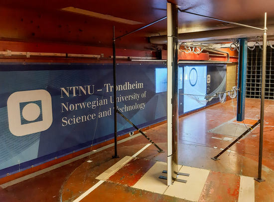
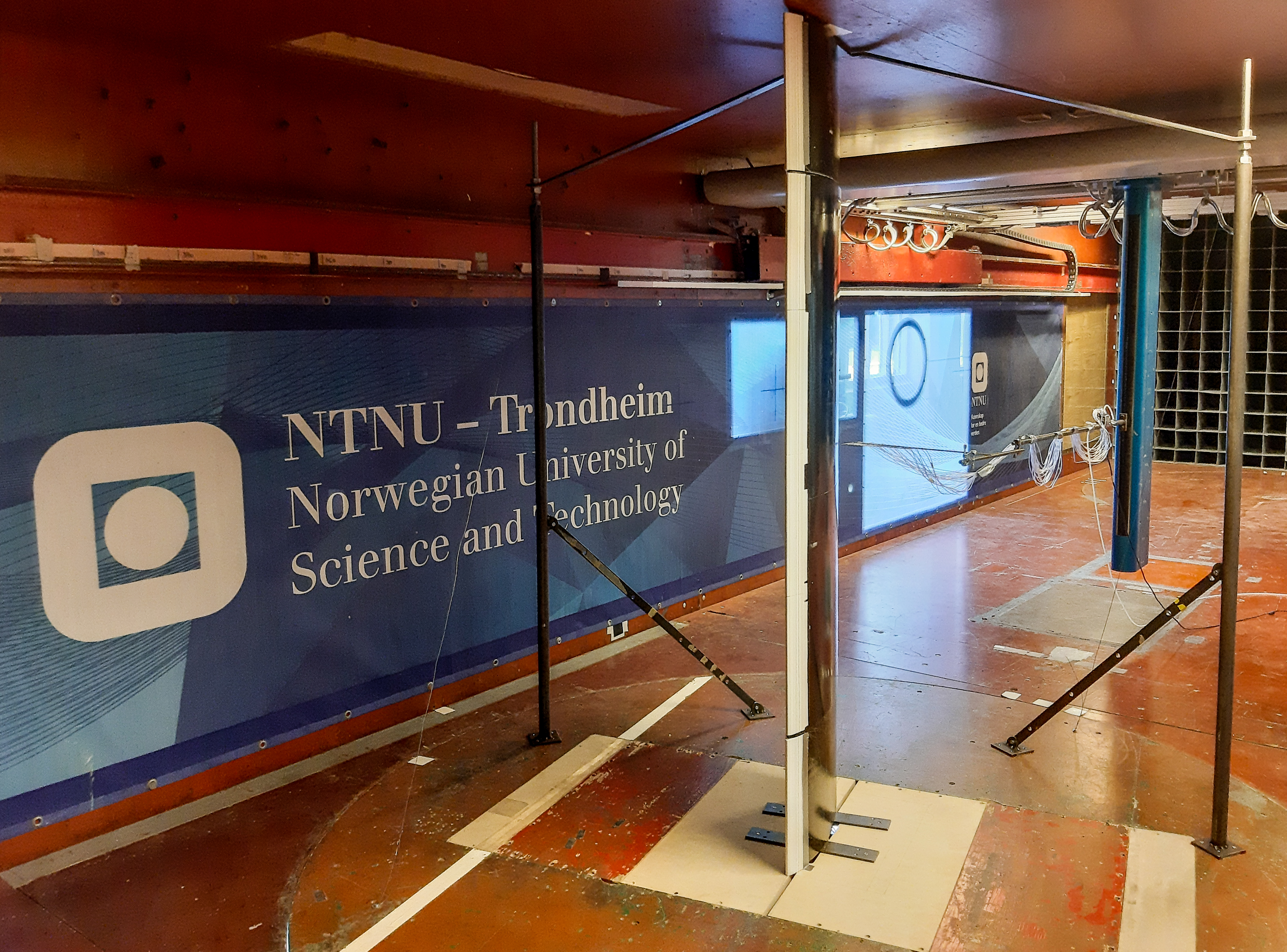
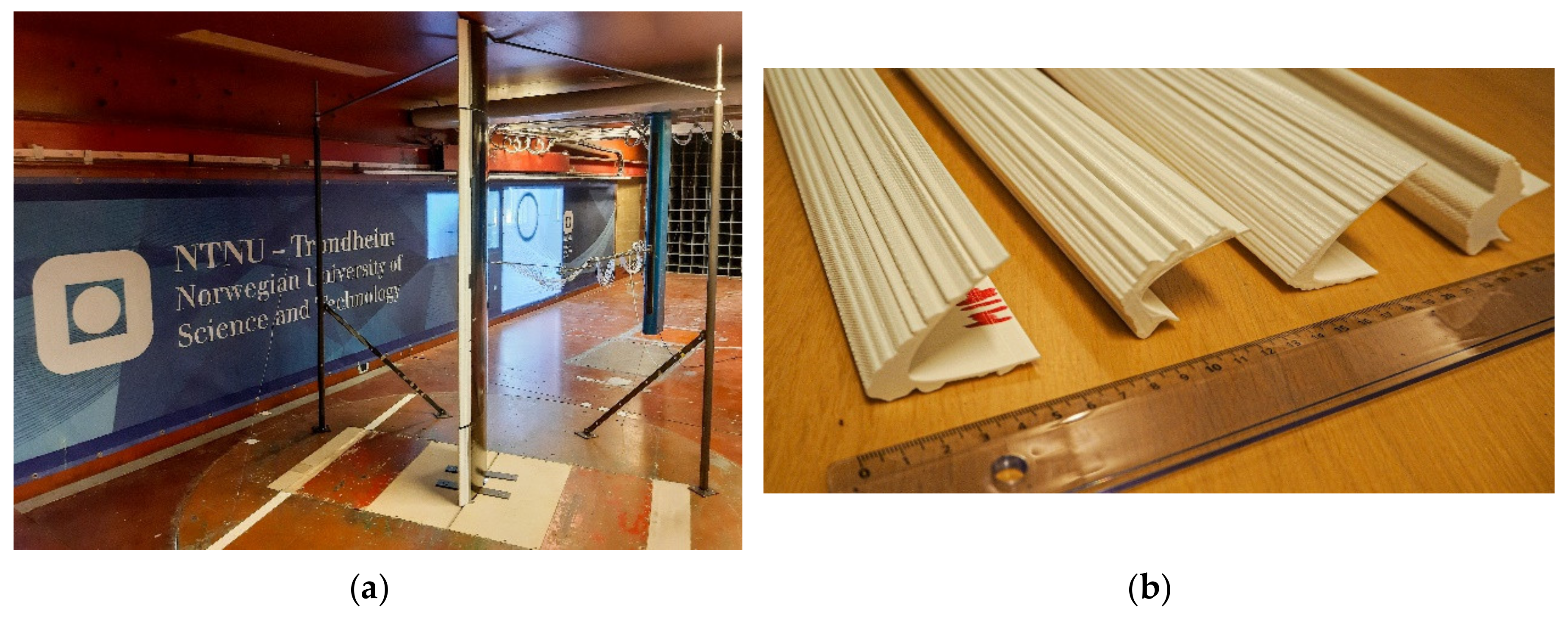
3. Experimental Setup

The experimental part of this work was performed in the closed-loop, low-speed wind tunnel at the Norwegian University of Science and Technology (NTNU). An NREL S826 airfoil with a chord of c = 0.45 m was used in this study. This work follows the experimental methods described by Bartl et al. and their extensive study on the clean S826 airfoil, previously at NTNU [32].
The dimensions of the wind tunnel test section are 1.8 m × 2.7 m × 12 m (height × width × length), with the height increasing to 1.85 m at the end of the test section to compensate for the boundary-layer growth of the wind tunnel walls. Measurements were conducted for angle of attacks (AOAs) ranging from α = −7.5–17.5° at three Reynolds numbers: Re = 2 × 10⁵, 4 × 10⁵, and 6 × 10⁵. The corresponding inflow turbulence intensities for each Reynolds number are I = 0.44%, 0.30%, and 0.26% [32].
Figure 2a shows the experimental setup, watching at the leading edge of the wing, which spans the whole wind tunnel height. The wing consists of two “dummy” parts near the tunnel walls and the main section. The total height is h = 1.78 m. Only the middle section was connected to a force balance. All wing elements were computer numerical control milled from Ebazell foam and coated with black paint. Surface roughness measurements confirmed that the surface was hydraulically smooth. The trailing edge thickness was 2 mm.
A six-axis force balance recorded the aerodynamic forces acting on the main wing section during a period of 30 s with a sampling rate of 2000 Hz. Two load cells were aligned with the flow direction of the wind tunnel and one was perpendicular to it. The results from Bartl et al. [32] showed that lift measurements could be accurately obtained with the force balance, but the accuracy was insufficient for drag estimations due to excessive signal-to-noise ratios. Instead, drag was measured with a wake rake using an integrated momentum deficit method. The rake is constructed with 21 uniformly distributed tubes of 1mm diameter, with 10mm spacing between the centerline of each tube. It was located at a distance of 0.7c downstream of the trailing edge, mounted on a traverse. All pressure ports were connected to a pressure scanner and were sampled for a duration of 20 s with a sampling rate of 200 Hz.
In addition, 32 pressure taps are located in the middle of the main section and connected to a piezoresistive pressure scanner inside the wing. The reference pressure is taken from the static pitot tube upstream of the wing. Surface pressure data were collected at a sampling rate of 800 Hz for 30 s. The artificial ice shapes covered the pressure taps near the leading edge up to x/c = 0.09–0.15 (depending on the coverage by the different ice shapes). Therefore, the pressure readings were not used for any force calculation, but only to calculate the local pressure coefficients. The flow velocity and the reference pressures for the wake rake and surface pressures were measured with a pitot-static tube at a distance of 5c upstream of the wing.
In order to change the angle of attack, the entire set-up, including the force balance, was mounted on a turntable with a rotational accuracy of ±0.25°. The largest blockage ratio occurring between the model and the flow cross-section was σmax = 5.1% at the highest angle of attack α = 18°. This was below the limit of σ = 10%, above which blockage correction needs to be considered [41]. Earlier investigations showed that small losses in static pressure between the upstream pitot probe and the downstream rake occurred. Measurements also showed that the static pressure at the location of the rake is not fully stabilized. Both these effects contribute to a reduction of the drag coefficients, which has been approximated to be in the order of up to 20% [32]. In addition, the wake rake measurements were only reliable as long as no strong separation effects occurred. This is because the rake cannot capture the resulting 3D velocity field. This means that for high angles of attack α > 12° for clean and α > 6–12° (depending on the ice shape) drag measurements from the wake rake were increasingly erroneous. More details on the general wind tunnel configuration and measurement method can be found with Bartl et al. [32].
Artificial ice shapes were 3D-printed via fused deposition modeling at NTNU in polylactide plastic, on an Ultimaker S5 and S2+ printer with a layer height of 100 μm, see Figure 2b. The artificial ice shapes cover the entire height of the wing, including the dummy sections, and were attached with tape.
In order to assess the influence of the laminar-turbulent transition, a series of runs were performed with a tripped boundary-layer. For this purpose, self-adhesive zig-zag tape, acting as a turbulator was applied to the upper and lower side of the leading edge at the location x/c = 0.05. The tape thickness was 0.4 mm with a width of 8 mm and a pattern angle of 60°.

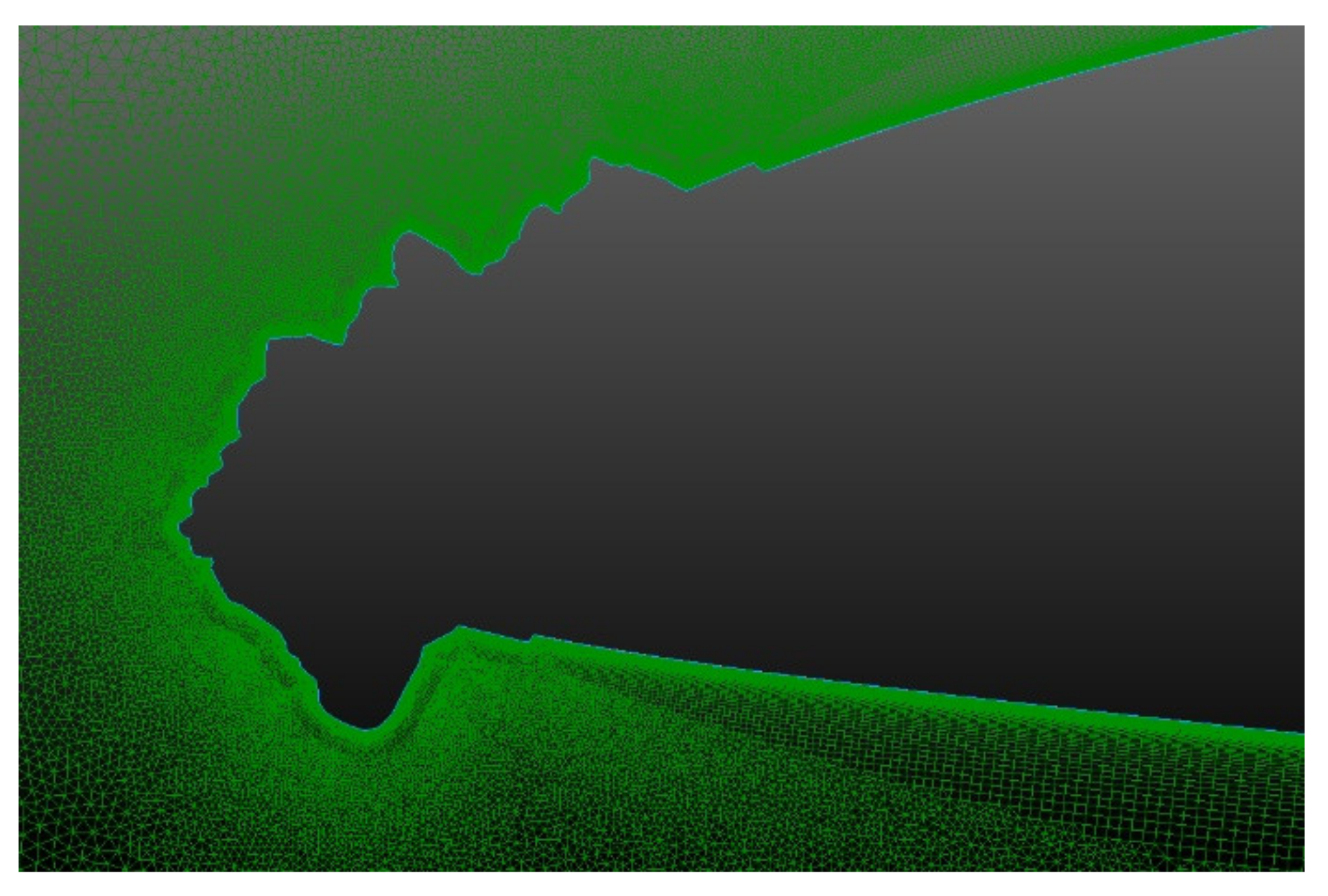
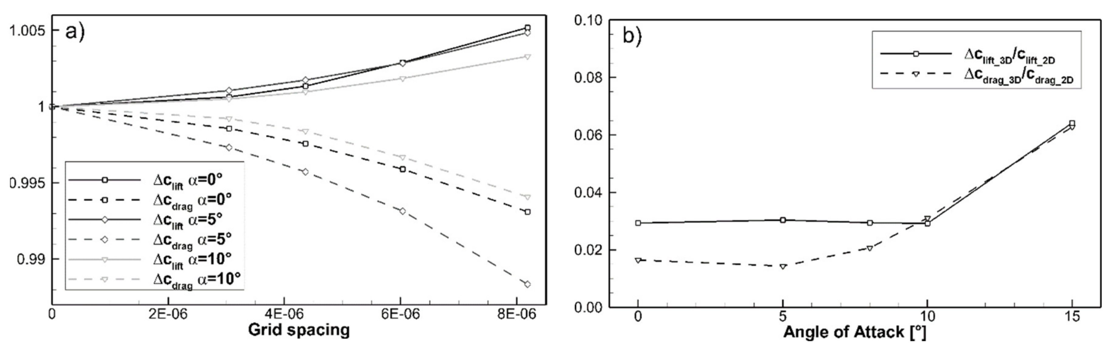
4. Numerical Methods

The aerodynamic performance degradation due to icing was simulated with FENSAP, a state-of-the-art Navier–Stokes CFD solver [42]. The solver is part of the software package ANSYS FENSAP-ICE (version 19.2) [43], which is a second generation icing simulation tool suitable for a wide range of applications but with limited published validation data—in particular, for low Reynolds numbers. One objective of this study was to use FENSAP as an example to compare it to the experimental dataset and assess its capability to capture icing performance penalties at low Reynolds numbers. All FENSAP calculations were run as steady-state 2D simulations with a streamline upwind artificial viscosity model. The airfoil geometries were discretized in Pointwise (version 18.2R2) as a hybrid O-grid with a far-field diameter of 60c. The boundary-layer was resolved with a structured 3D anisotropic tetrahedral extrusion (T-Rex) with a growth factor of 1.1 [44]; see Figure 3.
The comparison consisted of three steps. First, the clean airfoil aerodynamics were simulated and compared to the experiments. One of the main challenges for the clean airfoil simulation is the laminar-turbulent transition. Two turbulence models were implemented in FENSAP [45]. The Spalart-Allmaras (SA) turbulence model is a classical one-equation model (eddy-viscosity), whereas the Menter’s k-ω SST model is a two-equation model (turbulence kinetic energy and eddy dissipation rate) [46]. For both these turbulence formulations, a transition model is available. For the SA model, free transition is captured based on adverse pressure gradients, whereas the Menter’s k-ω SST model uses a one-equation local correlation-based intermittency transition mode [45].
The second comparison step was to ensure that the chosen numerical discretization (grid) of the iced airfoils did not significantly affect the results. For this, a 2D grid convergence study was performed in order to find a grid resolution that was sufficiently accurate while optimizing computational power and time. The grid dependency study was performed on four grid resolutions, at three different angles of attack α = [0°, 5°, 10°] on one of the ice shapes (glaze ice, see Section 5.2). The results are shown in Figure 4a with the drag and lift coefficients normalized by a Richardson extrapolation ∆clift = clift/clift,Richardson and cdrag = cdrag/cdrag,Richardson [47]. The results showed good convergence for lift and drag for all angles of attack. In order to limit the computational requirements for this study, the second-coarsest grid (ca. 170,000 points) was used for all subsequent simulations.
The third comparison step consisted of a study to compare the differences between the 3D constrained flow in the wind tunnel to the 2D simulations. For this purpose, the entire wind tunnel and test section was modelled in 3D. Lift and drag forces were calculated on the main wing section, excluding the dummy parts. Figure 4b compares the simulated 3D results to the 2D solution with ∆c3D/2D = [c3D/c2D − 1] for five angles of attack. The results show that for angles of attack up till α = 10° the difference between the 2D and the 3D solution is about 3% and increases to about 7% for the highest angle of attack. These deviations are assumed to be comparatively minor and justify the use of 2D simulations (e.g., [48]).

5. Experimental Results

This section presents the experimental measurements of lift and drag from the NTNU wind tunnel for the two types of ice shapes. In addition, the influence of the small-scale surface roughness was investigated by comparing the (rough) IWT ice shapes to smooth ice shapes.

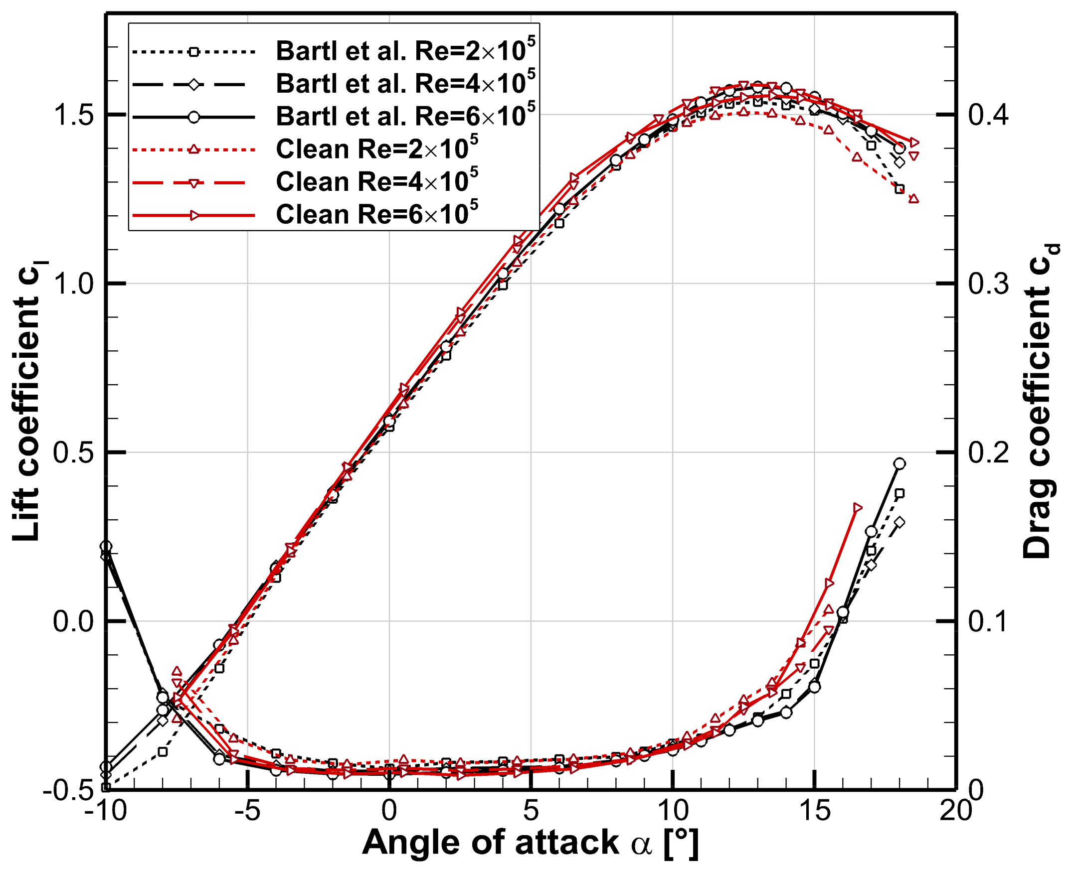
5.1. Comparison to Existing Data
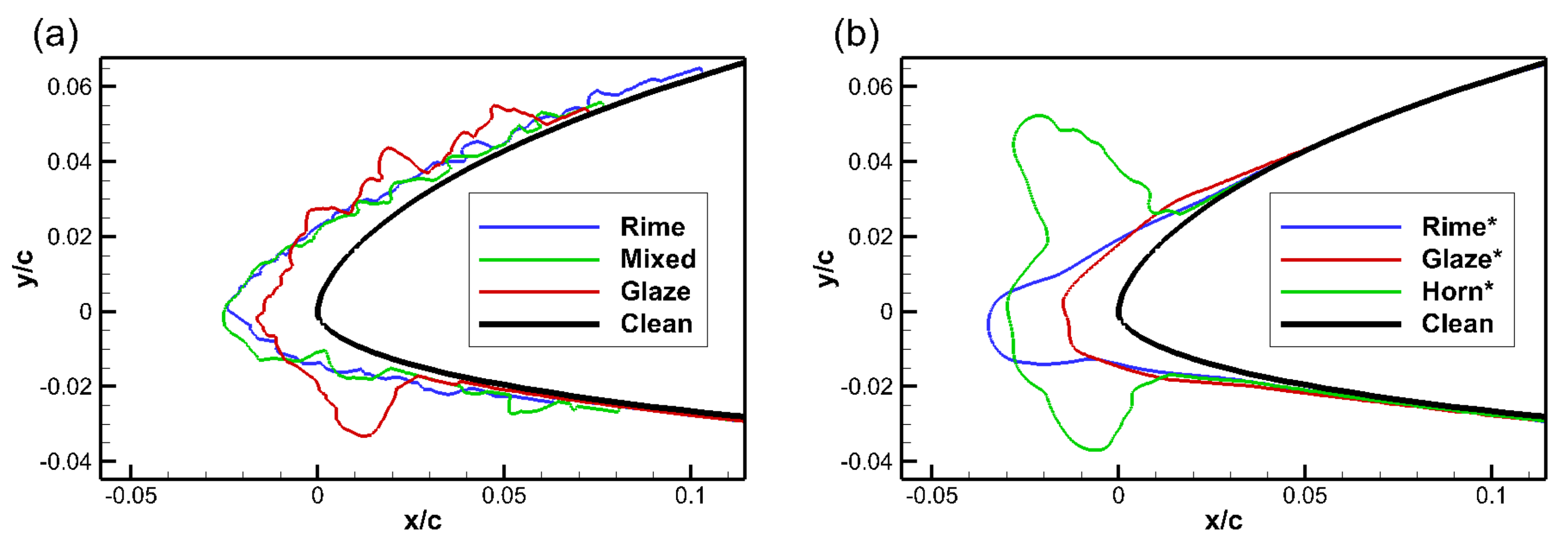
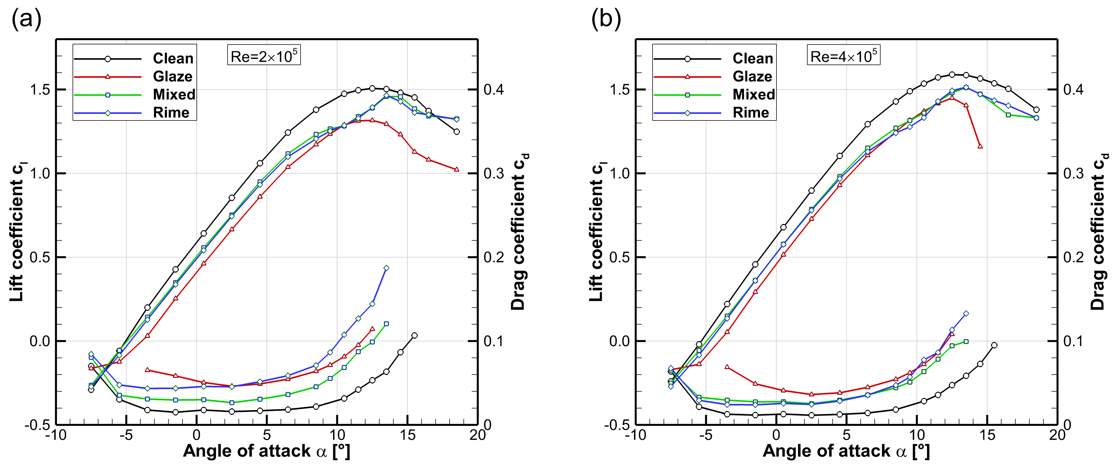
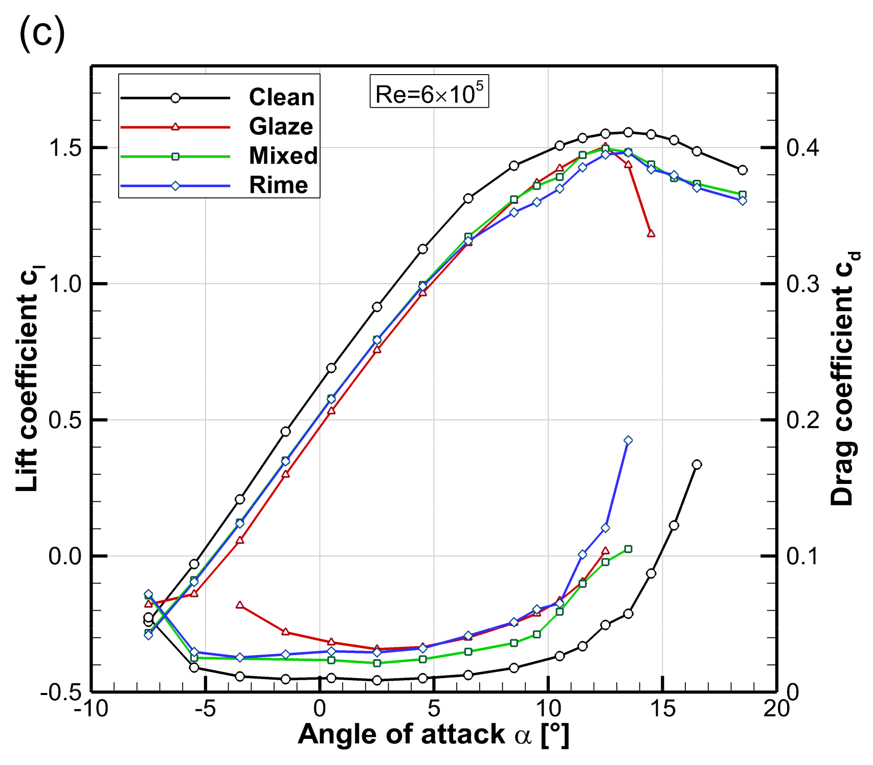
Figure 5 compares the experimental lift and drag results for the clean airfoil from this study to the results from Bartl et al. [32]. In general, the datasets are in good agreement, which is not surprising because identical facilities and methods were used. The largest deviations occurred in the stall area, particularly for drag, which is most likely related to the high measurement uncertainty of the wake rake in that area. The small level of Reynolds-dependency for Re = 2–6 × 10⁵ that was observed by Bartl et al., was also reproduced in this work. The decision to investigate three Reynolds numbers in this work was based on the possibility that iced airfoils may show a higher degree of Reynolds dependency. In conclusion, the good match between the clean curves gives us confidence that the experimental setup was accurate, and that data are repeatable.

5.2. IWT Ice Shapes

The lift and drag results for the three experimental IWT ice shapes are shown in Figure 6a–c in comparison to the clean airfoil. The first observation was that all ice shapes introduced significant penalties on lift and drag. Lift decreased and drag increased over the entire range of angles of attack values. The degree of degradation depended on the ice shape type. The low Reynolds number results generally showed higher drag levels and lower lift for both clean and iced airfoils.
The glaze ice shapes gave the largest penalties. For zero angle of attack, the lift was decreased between ∆cl = −26–31% and drag was increased by ∆cd = +220–290%, as a function of the Reynolds number. The stall angle seemed unaffected, but the maximum achievable lift and the drag were both substantially reduced. Furthermore, the stall behavior was more aggressive, with a rapid loss of lift, especially for the higher Reynolds numbers.
For rime ice the degree of degradation was smaller with ∆cl = −17–19% and ∆cd = +100–190% at zero angle of attack. The drag curve at the lowest Reynolds number showed a significant increase compared to the other drag curves. In addition, the stall region showed an irregular behavior. The linear lift region ends at around α ≈ 7° with an apparent onset of stall. However, at about α ≈ 11° lift was suddenly increased, reaching a maximum at α ≈ 13–14° before showing a docile lift decrease. This uncharacteristic behavior occurred at all Reynolds numbers but was most distinct at the lowest Reynolds number. Potential explanations for this will be addressed in the discussion section.
Last, mixed ice exhibited the lowest performance penalties with ∆cl = −15–18% and ∆cd = +80–130% at a zero angle of attack. In the stall region, the same unexpected behavior with a sudden lift increase was observed, similarly to the rime case. This lift behavior showed a dependency on the Reynold number and decreased in distinction at higher Reynolds numbers.

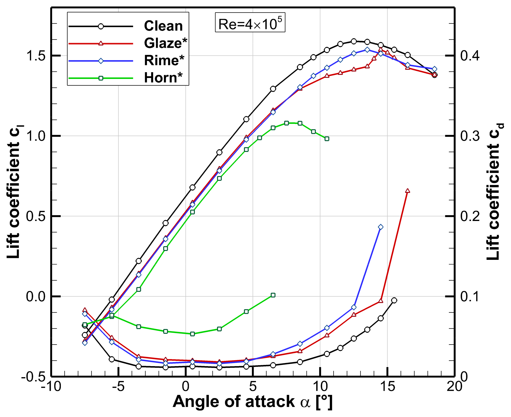
5.3. LEWICE Ice Shapes

The experimental results for the ice shapes obtained from LEWICE simulations are shown in Figure 7. Due to time limitations and because the IWT ice shapes did not show a major Reynolds number dependency, the LEWICE ice shapes were conducted only at Re = 4 × 10⁵. The largest penalties occurred for the horn* ice shape. At zero angle of attack, lift was decreased by ∆cl = −26% and drag more than quadrupled with an increase of ∆cd = +330%. The maximum lift angle occurred significantly earlier compared to the clean airfoil, at α ≈ 7°.
The rime* and glaze* ice shapes showed similar degrees of degradation in both lift and drag with ∆cl = −16–17% and ∆cd = +40–60% at zero angle of attack. Differences showed up in the stall region, where the glaze ice shape displayed a similar lift behavior as the IWT rime and mixed ice shapes. However, in this case, the lift increase arose significantly later, at α ≈ 14° and the maximum lift was reached at α ≈ 15°. The rime ice shape exhibited a normal stall behavior

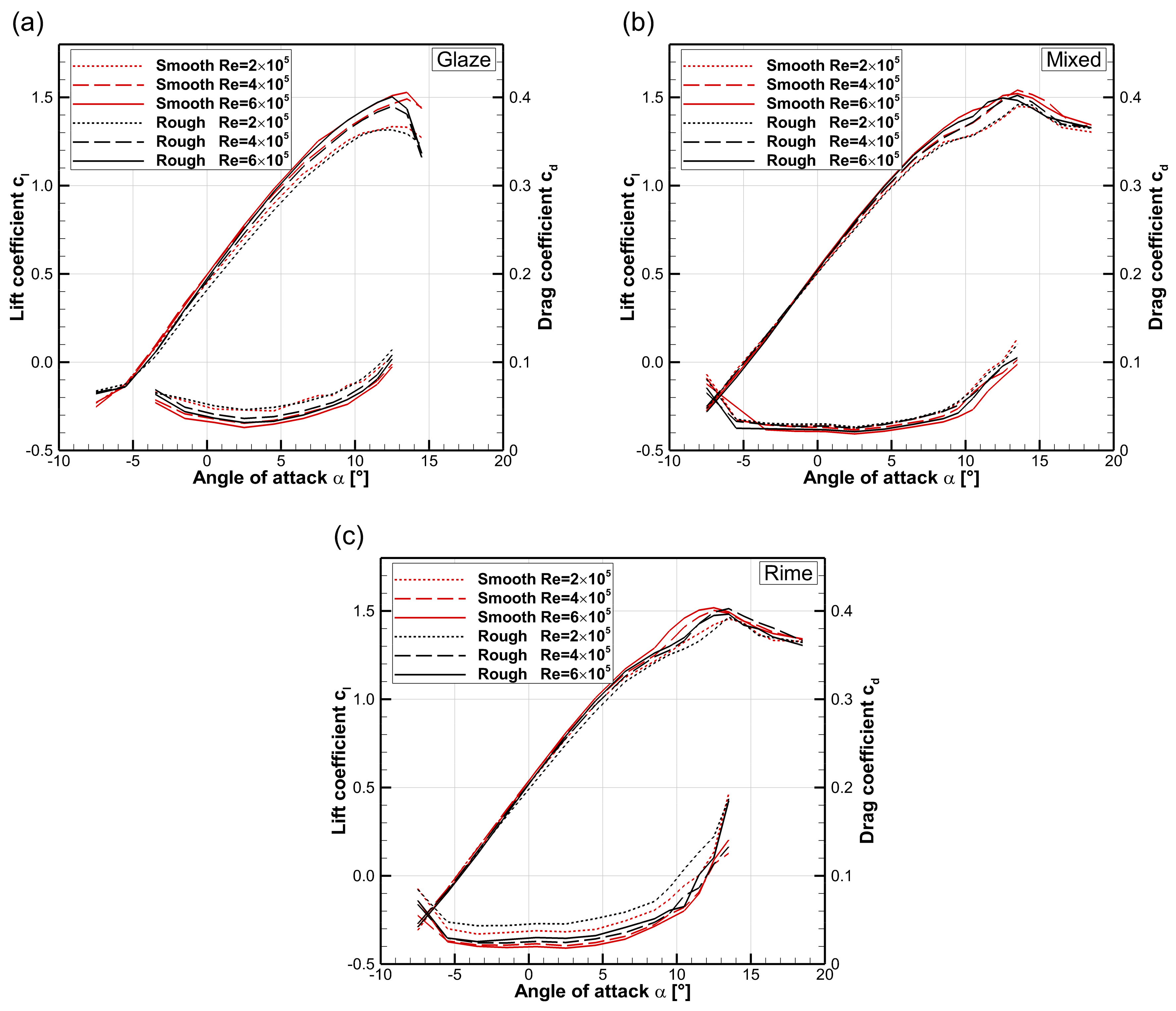
5.4. Influence of Roughness

Figure 8 shows the comparison of smooth and rough IWT ice shapes to highlight the influence of the small-scale roughness. The general trend that was observed for all lines is that the additional surface roughness led to a decrease in lift and an increase in drag.
For the glaze ice shapes, the smooth surfaces seemed to delay the maximum stall angles by ∆α ≈ 1° while increasing the maximum lift slightly. The sudden lift increase in the stall region of the rime and mixed ice shapes prevailed in the absence of the surface roughness. The results indicated that the effect may be slightly more pronounced for the rough airfoils, especially for rime ice.

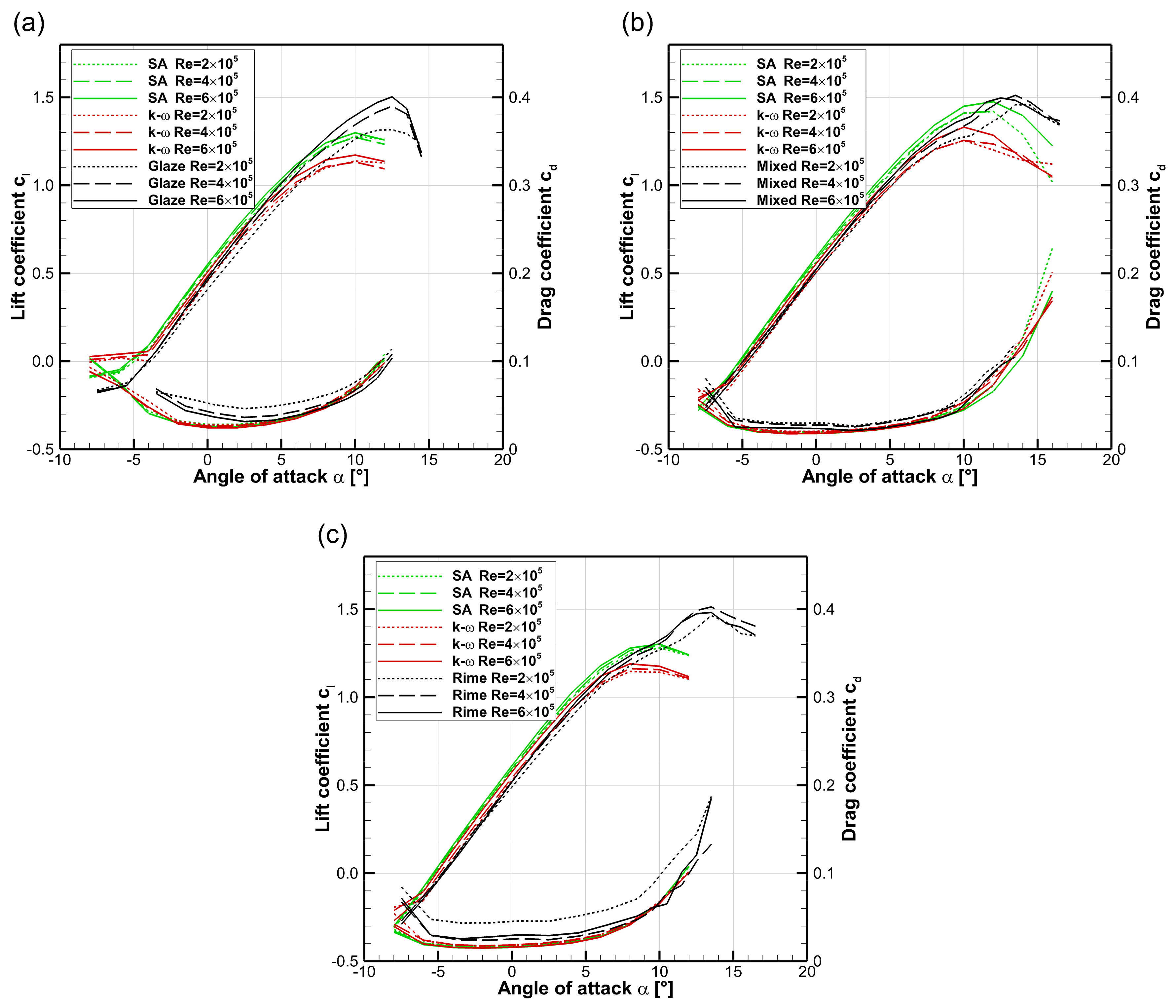
6. Simulation Results

This section presents the numerical simulation results from FENSAP in comparison to the experimental measurements. In addition to the two types of ice shapes, the simulations were also conducted on the clean airfoil.

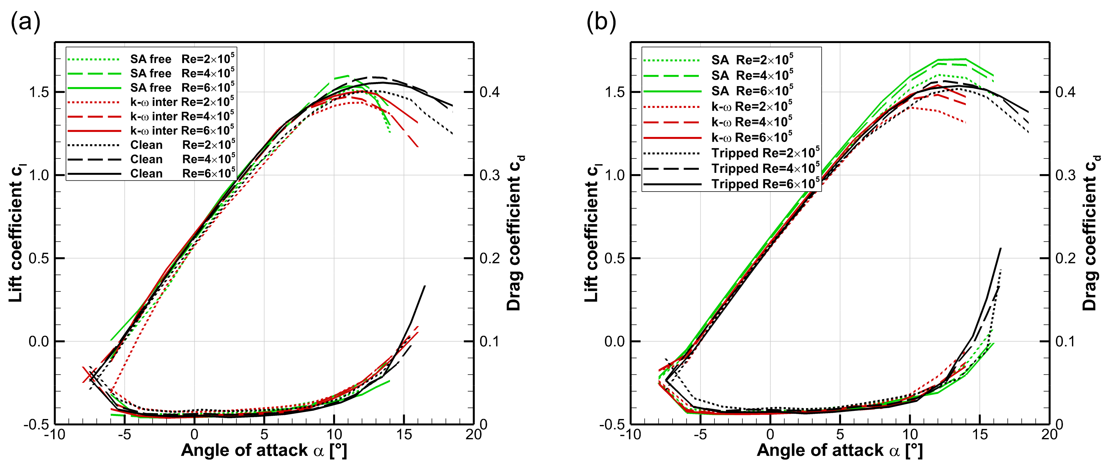
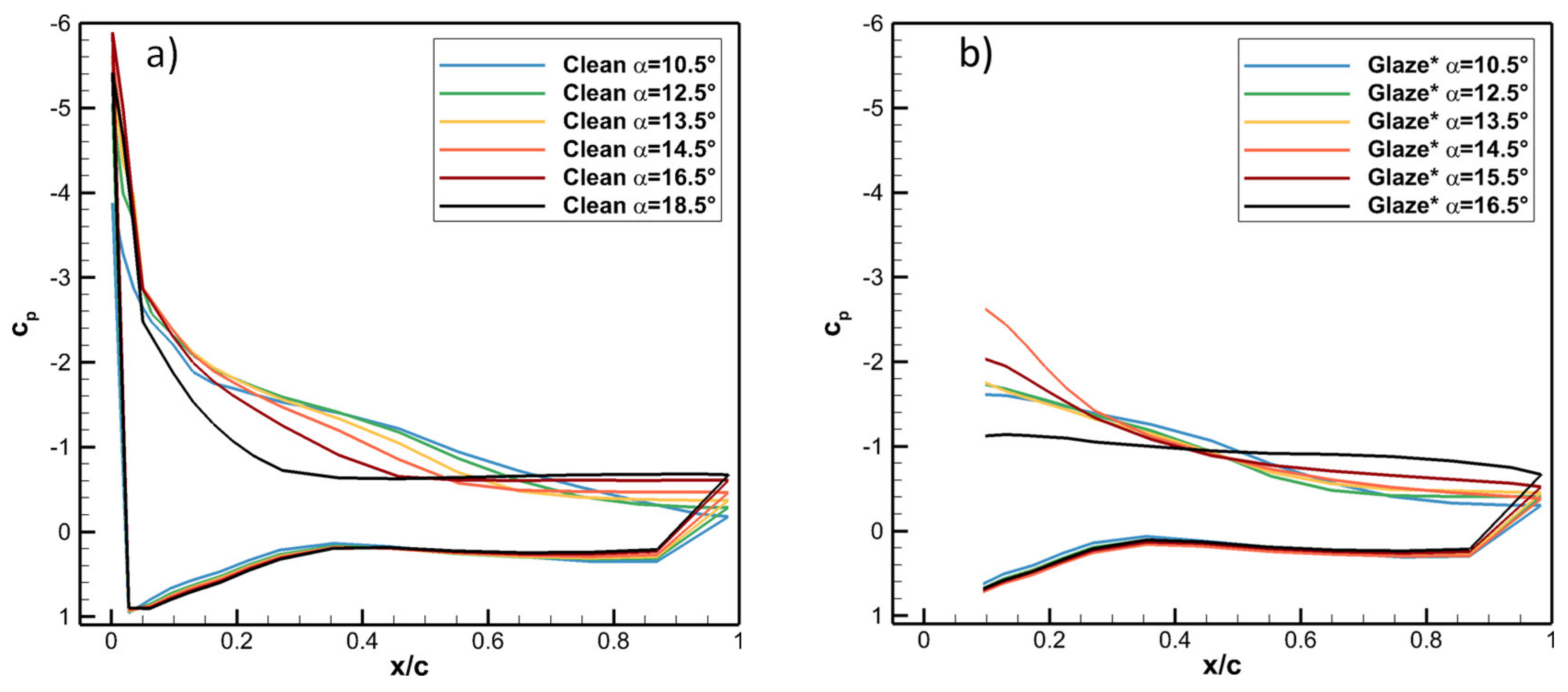
6.1. Clean and Tripped
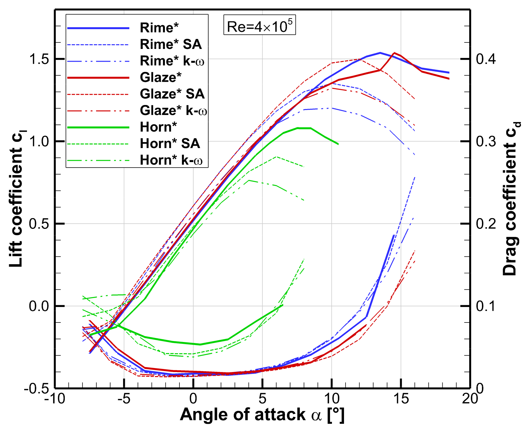
The first simulations aimed to establish that the clean airfoil aerodynamics could be captured accurately. Figure 9a shows the results for the clean airfoil with free transition and numerical results with transition modeling. Both turbulence models seemed to capture the experimental results with a good degree of accuracy. Lift and drag values in the linear region showed a good overlap at all Reynolds numbers. Notable differences occurred in the stall region, where both turbulence models failed to reproduce the experimental stall behavior. Generally, the numerical results predicted the maximum lift angle about ∆α ≈ 2° earlier than the experiments and also with a more aggressive stall behavior. The k-ω SST model tended to predict lower maximum lift levels, whereas the SA model resulted in a maximum lift comparable to the experiments. Drag was captured in all cases with good accuracy, although deviations occurred in the stall region due to earlier predicted stall from the numerical models.
In addition, an experimental run with a forcibly tripped boundary at x/c = 0.05 was conducted to be able to compare it to fully-turbulent numerical simulations; see Figure 9b. Compared to the experiments with free transition, the tripped runs exhibited slightly lowered levels of lift and increased levels of drag. Stall and the maximum lift angle were marginally delayed. The fully-turbulent numerical results showed that both turbulence models slightly overpredicted the lift in the linear region, whereas drag seemed to be captured well. The fully-turbulent SA model estimated significantly higher maximum lift values in the stall region with a slightly earlier stall. In contrast, the fully turbulent k-ω SST model predicted the maximum lift value well but showed stall at earlier angles of attack and also more aggressive stall behavior.

6.2. IWT Ice Shapes

Figure 10a–c shows the comparison between the experimental and the computational results. For glaze ice, the simulation results of lift and drag exhibited a constant offset. The lift simulations in the linear area were shifted to lower angles of attack with an offset of ∆α ≈ 0.3–0.8° for the k-ω SST/SA models. Maximum stall angles were captured better with the SA model than k-ω SST, but both predicted the maximum stall angle ∆α ≈ 2° earlier compared to the experiments. The numerical drag predictions gave significantly lower results compared to the experiments, particularly for α < 4°. The numerical results also indicated a substantially lower effect of the Reynolds number, compared to the experiments.
The mixed ice experimental results had a better overlap between the simulations and the experiments. In the linear lift section, both turbulence models tended to predict higher lift and lower drag compared to the experiments. In the stall region, the k-ω SST model showed the maximum lift with a significantly lower lift value and at lower angles of attack. The SA model seemed to capture the stall behavior better, with maximum lift and stall angle closer to the experiments. However, none of the simulation results reproduced the sudden lift increase in the experimental results, starting at α ≈ 11°.
The simulation results for rime ice showed a similar trend as for mixed ice, with larger levels of deviations, however. In the linear region, the simulations predicted higher lift values and significantly lower drag. None of the turbulence models captured either the stall angle or the maximum lift value correctly. Again, the unusual behavior of the sudden lift increase in the stall region was not reproducible with the numeric methods.

6.3. LEWICE Ice Shapes
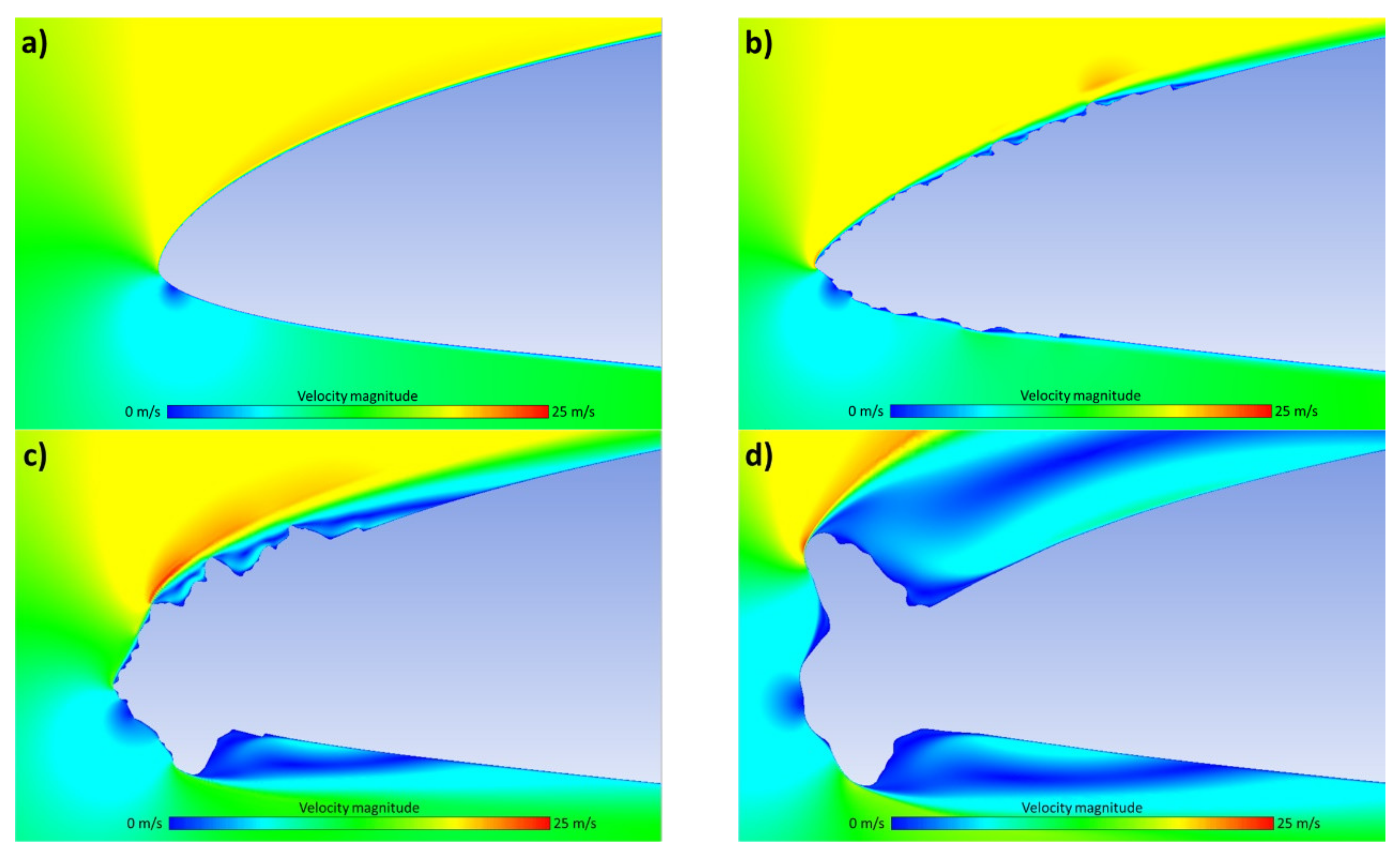
The simulation results for the ice shapes generated by LEWICE are shown in Figure 11. For rime* ice, the SA model predicted higher lift in the linear region and an earlier stall angle—however, the maximum lift was matched well. The k-ω SST model matched lift in the linear region but predicted earlier stall at lower maximum lift. For drag, both turbulence models matched the experiments well. The glaze* ice results showed similar trends. The main difference, however, was that the sudden lift increase at α ≈ 14° was not captured by the numerical simulations. The simulations of the horn* ice shapes predicted lower lift, particularly in the stall region. Furthermore, the drag results from the numerical models were substantially lower compared to the experiments. Both these effects may be related to the significant separation zones induced by the ice horns.

7. Discussion

7.1. Experiments

In general, the experiments showed that the performance degradation is linked to the geometry of the ice shape. The largest differences between the results can be observed for the drag curves. The most streamlined ice shapes (glaze* and rime*) resulted in the smallest increases in drag, compared to the more complex IWT ice shapes. The largest drag penalties occurred for the glaze and horn* ice shapes, which can be explained by the large horn geometry that resulted in large separation bubbles. The correlation between performance degradation and ice shape geometry can also be detected for lift. In the linear lift region, this effect is less obvious, but it can be observed for the stall behavior—especially for glaze and horn*, which exhibited earlier stall, lower maximum lift, and rapid lift decrease.
The variation of the Reynolds numbers seemed to have a lesser effect on the results. The general trends were that higher Reynolds numbers led to increased lift and a decrease in drag levels. One notable occurrence was found for the rime ice shape at Re = 2 × 10⁵, where the drag was increased substantially compared to the higher Reynolds numbers. This can most likely be linked to the relatively high measurement uncertainties related to the small forces acting on the measurement balance.
A surprise from the experimental data was the stall behavior occurring for the IWT mixed, IWT rime, and the LEWICE glaze* ice shapes. In all these cases, a sudden lift increase occurred in the stall region. A measurement error was very unlikely, as this effect was reliably reproduced for the ice shapes in question. No unsteady behavior was found, either in the force balance measurements or the pressure tap data. The effect showed a slight tendency to decrease for higher Reynolds numbers; see Figure 8b–c.
To investigate the stall behavior, the pressure distributions over the clean and an iced airfoil were examined. Figure 12a displays the distribution of the pressure coefficient cp over the clean airfoil and shows how the stall was starting from the trailing-edge. For the iced airfoil, the LEWICE glaze* case was investigated, since it showed the clearest lift increase behavior; see Figure 7. The glaze* pressure distribution in Figure 12b showed that the additional lift seemed to originate from the leading-edge, where increased suction pressure occurred at x/c < 0.3 for α = 13.5–15.5°.
One hypothesis for the origin of this increase in leading-edge suction is an increase of the airfoil camber. According to this idea, the initial break in the lift curve (α ≈ 9°) occurs due to the onset of trailing-edge separation. The lift increase (α ≈ 14°) would originate either from the ice shape acting as a nose droop [49], or possibly, from a localized separation bubble [50]. This effect would decrease at higher Reynolds numbers because the onset of the trailing-edge separation moves to higher angles of attack due to the higher boundary-layer inertia. This would explain why this effect has not been observed on a wider scale for high-Reynolds applications. Comparable effects have indeed been documented before at low Reynolds numbers by Jasinski et al., who suggested a “leading-edge flap”-like behavior as an explanation, ([23], pp. 61–62). Additionally, a lesser degree lift increase occurs in Seifert and Richert’s experiments, without them addressing it explicitly ([22], pp. 459–460).
The exact mechanism of the unexpected stall behavior could not be fully proven within the scope of this work. To test the hypothesis, flow visualization techniques, wider Reynolds number range, moment measurements, and pressure measurements on the ice shapes should be conducted in follow-up studies.

7.2. Simulations

The experimental results were qualitatively compared to FENSAP, using the SA and k-ω SST turbulence models. For the clean airfoil with free transition and tripped boundary-layer, both turbulence models showed a good match in lift and drag with the experiments and were able to reproduce the linear drag behavior of the airfoil. Larger differences occur in the stall regions, where both models did not capture the experimental stall behavior. The SA model tended to predict higher lift values, whereas the k-ω SST tended to predict lower maximum lift angles and earlier stall.
The quality of the lift and drag prediction of iced airfoils appeared to depend on the ice shape. For the most streamlined cases (LEWICE rime* and glaze*) both turbulence models captured the drag well. In the linear lift region, the k-ω SST model seemed to match the experiments better, whereas the SA model tended to overpredict the lift. The stall behavior was not captured well by either of the turbulence models, resulting in an earlier stall and lower maximum lift values. This was likely to be related to the shortcomings of the turbulence models in the presence of large separation zones [46]. For the more rugged shapes of the IWT rime and mixed ice shapes, the codes behaved similarly, with exception to the drag results, which were significantly lower compared to the experiments. This was likely to be related to the ruggedness of the surface and the inability of the turbulence models to capture the associated drag increase. This trend amplifies for the more complex ice shapes of glaze and horn*, where the large separation areas also occurred in the linear lift region; see Figure 13a–d.
The unexpected stall behavior of some of the ice shapes was not captured by the simulation with any of the turbulence models. This was not entirely surprising and was most likely related to the limitations of the SA and k-ω SST turbulence models. Further work should investigate the possibility of 3D flow effects, transient flow behavior, and the use of higher-order models.
In summary, the comparison between FENSAP and the experimental data showed that even CFD-RANS can be used to get reasonable lift and drag predictions at low Reynolds numbers. Limitations seem to exist in the stall area and for complex ice shapes with large leading-edge separation zones. Consequently, FENAP may be suited, for example, to predict intercycle ice penalties for the design of de-icing systems at low Reynolds numbers [51]. Similarly, effects on wind turbine power production or UAV flight behavior may be simulated with sufficient accuracy with FENSAP.

8. Conclusions

This study conducted experimental and numerical investigations on the performance degradation of an S826 airfoil with 3D printed ice shapes at low Reynolds numbers. The experimental data of this work are shared as Supplementary Materials and are suitable to be used for the validation of other numerical tools for the prediction of icing penalties at low Reynolds numbers. The experimental results showed that the overall degree of performance penalties being due to icing is correlated with the geometry of the ice shapes. Rough, rugged, and complex geometries resulted in higher aerodynamic performance degradation in the form of increased drag, decreased lift, and earlier stall. The experiments were compared CFD flow solver FENSAP with two turbulence models. The fidelity of the results was linked to the geometry of the ice shapes. The ice shapes that resulted in higher penalties had the largest discrepancies between the experiments and the simulations. This was most likely related to limitations of the turbulence models. For some ice shapes, an unexpected lift behavior was observed in the stall region. This was hypothesized to be related to a local increase in camber. This effect may be related to similar behaviors observed in the literature before, and is likely to be an aerodynamic effect related to low Reynolds numbers.

Supplementary Materials

The ice shape geometries and the experimental results are available online at https://www.mdpi.com/2226-4310/7/4/46/s1.

Author Contributions

Conceptualization, all authors.; methodology, R.H. and T.B.; software, R.H.; validation, R.H. and T.B.; formal analysis, R.H. and T.B.; investigation, R.H. and T.B.; resources, L.R.S.; writing—original draft preparation, R.H.; writing—review and editing, all authors; visualization, R.H.; supervision, R.J.H. and L.R.S.; project administration, R.H. All authors have read and agreed to the published version of the manuscript.

Funding

This project has received funding from the Research Council of Norway under grant number 237906, Centre for Integrated Remote Sensing and Forecasting for Arctic Operations (CIRFA). The research was also funded by grant number 223254, Centre for autonomous marine operations and systems (NTNU AMOS). The numerical simulations were performed on the Vilje supercomputer, Notur/NorStore project code NN9613K.

Acknowledgments

We thank Andy P. Broeren (NASA Glenn) for his valuable contributions to the discussion of the unexpected stall behavior. Furthermore, we thank Jan Bartl (HVL) for his support and advice for setting up the wind tunnel experiments.

Conflicts of Interest

The authors declare no conflict of interest.

References

  1. Bragg, M.B.; Broeren, A.P.; Blumenthal, L.A. Iced-airfoil aerodynamics. Prog. Aerosp. Sci. 2005, 41, 323–362. [Google Scholar] [CrossRef]
  2. Gent, R.W.; Dart, N.P.; Cansdale, J.T. Aircraft icing. Philos. Trans. R. Soc. Lond. Ser. A Math. Phys. Eng. Sci. 2000, 358, 2873–2911. [Google Scholar] [CrossRef]
  3. Leary, W.M. We Freeze to Please: A History of NASA’s Icing Research Tunnel and the Quest for Flight Safety; National Aeronautics and Space Administration: Washington, DC, USA, 2002. [Google Scholar]
  4. Wright, W.; Rutkowski, A. Validation Results for LEWICE 2.0; NASA Technical Report NASA/CR—1999-208690; NASA Center for Aerospace Information: Hanover, MD, USA, 1999. [Google Scholar] [CrossRef] [Green Version]
  5. Addy, H.E. Ice Accretions and Icing Effects for Modern Airfoils; Technical Publication NASA/TP--2000-210031; NASA Center for Aerospace Information: Hanover, MD, USA, 2000. [Google Scholar]
  6. Battisti, L. Wind Turbines in Cold Climates; Springer: Berlin/Heidelberg, Germany, 2015. [Google Scholar]
  7. Wallenius, T.; Lehtomäki, V. Overview of cold climate wind energy: Challenges, solutions, and future needs. Wires Energy Environ. 2016, 5, 128–135. [Google Scholar] [CrossRef]
  8. McTavish, S.; Feszty, D.; Nitzsche, F. Evaluating Reynolds number effects in small-scale wind turbine experiments. J. Wind Eng. Ind. Aerodyn. 2013, 120, 81–90. [Google Scholar] [CrossRef]
  9. Wood, D. Small Wind Turbines; Springer: Berlin/Heidelberg, Germany, 2011. [Google Scholar]
  10. Leary, J.; Schaube, P.; Clementi, L. Rural electrification with household wind systems in remote high wind regions. Energy Sustain. Dev. 2019, 52, 154–175. [Google Scholar] [CrossRef]
  11. Probst, O.; Martínez, J.; Elizondo, J.; Monroy, O. Small Wind Turbine Technology. In Wind Turbines; Al-Bahadly, I., Ed.; IntechOpen: London, UK, 2011. [Google Scholar]
  12. Carbon Trust. Small-Scale Wind Energy Policy Insights and Practical Guidance; Report; Carbon Trust: London, UK, 2008. [Google Scholar] [CrossRef]
  13. Feng, F.; Li, S.; Li, Y.; Tian, W. Numerical simulation on the aerodynamic effects of blade icing on small scale Straight-bladed VAWT. Phys. Procedia 2012, 24, 774–780. [Google Scholar] [CrossRef] [Green Version]
  14. Shu, L.; Liang, J.; Hu, Q.; Jiang, X.; Ren, X.; Qiu, G. Study on small wind turbine icing and its performance. Cold Reg. Sci. Technol. 2017, 134. [Google Scholar] [CrossRef]
  15. Siquig, A. Impact of Icing on Unmanned Aerial Vehicle (UAV) Operations; Naval Environmental Prediction Research Facility Report; Naval Environmental Prediction Research Facility: Monterey, CA, USA, 1990. [Google Scholar]
  16. Williams, N.; Benmeddour, A.; Brian, G.; Ol, M. The effect of icing on small unmanned aircraft low Reynolds number airfoils. In Proceedings of the 17th Australian International Aerospace Congress (AIAC), Melbourne, Australia, 26–28 February 2017. [Google Scholar]
  17. Szilder, K.; Yuan, W. In-flight icing on unmanned aerial vehicle and its aerodynamic penalties. Prog. Flight Phys. 2017, 9, 173–188. [Google Scholar] [CrossRef]
  18. Fajt, N.; Hann, R.; Lutz, T. The Influence of Meteorological Conditions on the Icing Performance Penalties on a UAV Airfoil. In Proceedings of the 8th European Conference for Aeronautics and Space Sciences (EUCASS), Madrid, Spain, 1–4 July 2019. [Google Scholar] [CrossRef]
  19. Hann, R.; Johansen, T. Unsettled Topics in UAV Icing; SAE Edge Research Report; SAE International: Warrendale, PA, USA, 2020. [Google Scholar]
  20. O’Meara, M.M.; Mueller, T.J. Laminar Separation Bubble Characteristics on an Airfoil at Low Reynolds Numbers. AIAA J. 1987, 25, 1033–1041. [Google Scholar] [CrossRef]
  21. Szilder, K.; McIlwain, S. In-Flight Icing of UAVs—The Influence of Reynolds Number on the Ice Accretion Process; SAE Technical Paper 2011-01-2572; SAE International: Warrendale, PA, USA, 2011. [Google Scholar] [CrossRef]
  22. Seifert, H.; Richert, F. Aerodynamics of Iced Airfoils and Their Influence on Loads and Power Production. In Proceedings of the European Wind Energy Conference, Dublin, Ireland, 6–9 October 1997. [Google Scholar]
  23. Jasinski, W.J.; Selig, M.S.; Bragg, M.B.; Shawn, C.N. Wind Turbine Performance Under Icing Conditions. J. Sol. Energy Eng. 1998, 120, 60–65. [Google Scholar] [CrossRef]
  24. Etemaddar, M.; Hansen, M.O.L.; Moan, T. Wind turbine aerodynamic response under atmospheric icing conditions. Wind Energy 2014, 17, 241–265. [Google Scholar] [CrossRef]
  25. Hochart, C.; Fortin, G.; Perron, J.; Ilinca, A. Wind turbine performance under icing conditions. Wind Energy 2008, 11, 319–333. [Google Scholar] [CrossRef]
  26. Han, Y.; Palacios, J.; Schmitz, S. Scaled ice accretion experiments on a rotating wind turbine blade. J. Wind Eng. Ind. Aerodyn. 2012, 109, 55–67. [Google Scholar] [CrossRef]
  27. Hudecz, A.; Koss, H.; Hansen, M.O.L. Ice Accretion on Wind Turbine Blades. In Proceedings of the 15th International Workshop on Atmospheric Icing of Structures (IWAIS XV), St. John’s, NL, Canada, 8–11 September 2013. [Google Scholar]
  28. Gao, L.; Liu, Y.; Hu, H. An experimental investigation on the dynamic ice accretion process over the surface of a wind turbine blade model. In Proceedings of the 9th AIAA Atmospheric and Space Environments Conference, Denver, CO, USA, 5–9 June 2017; pp. 1–18. [Google Scholar] [CrossRef] [Green Version]
  29. Knobbe-Eschen, H.; Stemberg, J.; Abdellaoui, K.; Altmikus, A.; Knop, I.; Bansmer, S.; Balaresque, N.; Suhr, J. Numerical and experimental investigations of wind-turbine blade aerodynamics in the presence of ice accretion. In Proceedings of the AIAA Scitech Forum, San Diego, CA, USA, 7–11 January 2019. AIAA 2019-0805. [Google Scholar] [CrossRef]
  30. Hansman, R.J.; Breuer, K.S.; Reehorst, A.; Vargas, M. Close-up Analysis of Aircraft Ice Accretion. In Proceedings of the 31st Aerospace Sciences Meeting and Exhibit, Reno, NV, USA, 11–14 January 1993. [Google Scholar]
  31. Somers, D.M. The S825 and S826 Airfoils; Technical Report NREL/SR-500-36344; U.S. Department of Energy: Oak Ridge, TN, USA, 2005. [Google Scholar]
  32. Bartl, J.; Sagmo, K.F.; Bracchi, T.; Sætran, L. Performance of the NREL S826 airfoil at low to moderate Reynolds numbers—A reference experiment for CFD models. Eur. J. Mech.-B/Fluids 2019, 75, 180–192. [Google Scholar] [CrossRef]
  33. Tiihonen, M.; Jokela, T.; Makkonen, L.; Bluemink, G. VTT Icing Wind Tunnel 2.0. In Proceedings of the Winterwind Conference, Åre, Sweden, 8–10 February 2016. [Google Scholar]
  34. Hann, R.; Borup, K.; Zolich, A.; Sorensen, K.; Vestad, H.; Steinert, M.; Johansen, T. Experimental Investigations of an Icing Protection System for UAVs. In SAE Technical Papers; SAE Technical Paper 2019-01-2038; SAE International: Warrendale, PA, USA, 2019. [Google Scholar] [CrossRef] [Green Version]
  35. Shin, J.; Bond, T.H. Experimental and computational ice shapes and resulting drag increase for a NACA 0012 airfoil. In Proceedings of the 5th Symposium on Numerical and Physical Aspects of Aerodynamic Flows, Long Beach, CA, USA, 13–15 January 1992. [Google Scholar]
  36. Wright, W. User’s Manual for LEWICE Version 3.2; NASA/CR—2008-214255; NASA Center for Aerospace Information: Hanover, MD, USA, 2008. [Google Scholar]
  37. Hann, R. UAV Icing: Comparison of LEWICE and FENSAP-ICE for Ice Accretion and Performance Degradation. In Proceedings of the Atmospheric and Space Environments Conference, Atlanta, GA, USA, 25–29 June 2018. AIAA 2018-2861. [Google Scholar] [CrossRef]
  38. Hann, R. UAV Icing: Ice Accretion Experiments and Validation. In SAE Technical Papers; SAE Technical Paper 2019-01-2037; SAE International: Warrendale, PA, USA, 2019. [Google Scholar] [CrossRef]
  39. Krøgenes, J.; Brandrud, L. Aerodynamic Performance of the NREL S826 Airfoil in Icing Conditions. Master’s Thesis, NTNU, Trondheim, Norway, 2017. [Google Scholar] [CrossRef] [Green Version]
  40. Federal Aviation Administration. 14 CFR Parts 25 and 29, Appendix C, Icing Design Envelopes; DOT/FAA/AR-00/30; U.S. Department of Transportation: Washington, DC, USA, 2002.
  41. Barlow, J.B.; Rae, W.H.; Pope, A. Low-Speed Wind Tunnel Testing; Wiley: Hoboken, NJ, USA, 1999. [Google Scholar]
  42. Habashi, W.G.; Morency, F.; Beaugendre, H. A Second Generation 3D CFD-Based In-Flight Icing Simulation System. In Proceedings of the FAA In-flight Icing / Ground De-icing International Conference & Exhibition, Chicago, IL, USA; 2003. [Google Scholar] [CrossRef]
  43. Reid, T.; Baruzzi, G.; Ozcer, I.; Switchenko, D.; Habashi, W.G. FENSAP-ICE Simulation of icing on wind turbine blades, part 1: Performance degradation. In Proceedings of the 51st AIAA Aerospace Sciences Meeting including the New Horizons Forum and Aerospace Exposition, Grapevine, TX, USA, 7–10 January 2013. AIAA 2013-0750. [Google Scholar]
  44. Steinbrenner, J.P. Construction of prism and hex layers from anisotropic tetrahedra. In Proceedings of the 22nd AIAA Computational Fluid Dynamics Conference, Dallas, TX, USA, 22–26 June 2015. [Google Scholar] [CrossRef]
  45. ANSYS. ANSYS FENSAP-ICE User Manual 18.2; ANSYS: Canonsburg, PA, USA, 2017. [Google Scholar]
  46. Blazek, J. Computational Fluid Dynamics: Principles and Applications; Butterworth-Heinemann: Oxford, UK, 2015. [Google Scholar]
  47. Roache, P.J. Quantification of Uncertainty in Computational Fluid Dynamics. Annu. Rev. Fluid Mech. 1997, 29, 123–160. [Google Scholar] [CrossRef] [Green Version]
  48. Sagmo, K.; Bartl, J.; Sætran, L. Numerical simulations of the NREL S826 airfoil. J. Phys. Conf. Ser. 2016, 753. [Google Scholar] [CrossRef]
  49. Ericsson, L.E.; Reding, J.P. Unsteady Airfoil Stall; NASA Report CR-66787; NASA Center for Aerospace Information: Hanover, MD, USA, 1969. [Google Scholar]
  50. Lissaman, P.B.S. Low-Reynolds-number airfoils. Annu. Rev. Fluid Mech. 1983, 15, 223–239. [Google Scholar] [CrossRef]
  51. Broeren, A.P.; Bragg, M.B.; Addy, H.E. Effect of intercycle ice accretions on airfoil performance. J. Aircr. 2004, 41, 165–174. [Google Scholar] [CrossRef]
Figure 1. Experimental ice shapes (a) and LEWICE ice shapes (b).
Aerospace 07 00046 g001
Figure 2. The wind tunnel set-up of the S826 consisting of dummy sections and the main part mounted vertically, with attached artificial ice shapes (a). The 3D printed ice shapes, from left to right: mixed, glaze, rime, and horn* (b).
Aerospace 07 00046 g002
Figure 3. Numerical T-Rex grid for the glaze ice shape, generated in Pointwise with a structured resolution of the boundary-layer and unstructured far field.
Aerospace 07 00046 g003
Figure 4. Grid dependency study on the 2D airfoil (a) and the fully resolved 3D wind tunnel (b).
Aerospace 07 00046 g004
Figure 5. Comparison of experimental results to Bartl et al. for Re = 2 × 10⁵, 4 × 10⁵, and 6 × 10⁵. Data adapted from [32].
Aerospace 07 00046 g005
Figure 6. Experimental results for lift and drag of the IWT ice shapes for Re = 2 × 10⁵ (a), 4 × 10⁵ (b), and 6 × 10⁵ (c).
Aerospace 07 00046 g006aAerospace 07 00046 g006b
Figure 7. Experimental results for lift and drag of the LEWICE ice shapes for Re = 4 × 10⁵.
Aerospace 07 00046 g007
Figure 8. Comparison of experimental results for lift and drag between the smooth and rough IWT ice shapes for glaze (a), mixed (b), and rime (c).
Aerospace 07 00046 g008
Figure 9. Comparison between numerical and experimental results of lift and drag for the clean (a) and the tripped (b) airfoil.
Aerospace 07 00046 g009
Figure 10. Comparison between numerical and experimental results of lift and drag for the IWT shapes of glaze (a), mixed (b), and rime (c).
Aerospace 07 00046 g010
Figure 11. Comparison between numerical and experimental results of lift and drag for the LEWICE ice shapes for Re = 4 × 10⁵.
Aerospace 07 00046 g011
Figure 12. Pressure coefficient distribution for the clean (a) airfoil and the glaze* ice shape (b).
Aerospace 07 00046 g012
Figure 13. FENSAP results for the velocity field of the clean (a), rime (b), glaze (c), and horn* (d) cases.
Aerospace 07 00046 g013
Table 1. Overview of existing data in the literature on airfoil performance degradation on iced airfoils at low Reynolds numbers.
SourceRe × 106AirfoilChordIcing CasesComments
Seifert & Richert, 1997 [22]0.6NACA44150.225 m4Unknown icing conditions. Ice shapes from fragments found near wind turbine.
Jasinski et al., 1998 [23]1.0–2.0S8090.457 m4Ice accretion from LEWICE.
Hochart et al., 2008 [25]0.3–0.7NACA63-4150.200 m6Performance data only at a single AOA.
Han et al., 2012 [26]1.0–1.4S8090.267 m17No performance data included in study.
Etemaddar et al., 2012 [24]2.0NACA64-6181.000 m2Ice accretion from LEWICE.
Hudecz et al., 2013 [27]1.0NACA64-6180.900 m3Performance data only at a single AOA.
Gao et al., 2017 [28]0.5DU96-W-1800.152 m6No performance data included in study.
Williams et al., 2017 [16]0.2RG-150.210 m4Low Reynolds number. Performance data from water and wind tunnel experiments.
Knobbe-Eschen et al., 2019 [29]2.3AH94W-1450.750 m2High Reynolds number.
This study0.4–0.8S8260.450 m6Ice shapes from IWT and LEWICE. Geometries and performance data shared.
Table 2. Overview of icing conditions used for the generation of the experimental icing wind tunnel (IWT) and LEWICE ice shapes.
ParameterIcing Wind Tunnel (IWT)LEWICE
GlazeMixedRimeGlaze*Horn*Rime*
SourceExperimentSimulation
v25 m/s25 m/s40 m/s25 m/s
T−2 °C−5 °C−10 °C−2 °C−4 °C−10 °C
MVD26 μm30 μm20 μm20 μm
LWC0.44 g/m³0.34 g/m³0.55 g/m³0.43 g/m³
ticing20 min40 min
αicing
c0.450 m
ks1.0 mm0.9 mm0.7 mm1.0 mm1.0 mm1.0 mm

