Computer-Assisted Aircraft Anti-Icing Fluids Endurance Time Determination

Abstract

Deicing and anti-icing the aircraft using proper chemical fluids, prior takeoff, are mandatory. A thin layer of ice or snow can compromise the safety, causing lift loss and drag increase. Commercialized deicing and anti-icing fluids all pass a qualification process which is described in Society of Automotive Engineering (SAE) documents. Most of them are endurance time tests under freezing and frozen contaminants, under simulated and natural conditions. They all have in common that the endurance times have to be determined by visual inspection. When a certain proportion of the test plate is covered with contaminants, the endurance time test is called. In the goal of minimizing human error resulting from visual inspection and helping in the interpretation of fluid failure, help-decision computer-assisted algorithms have been developed and tested under different conditions. The algorithms are based on common image processing techniques. The algorithms have been tested under three different icing conditions, water spray endurance test, indoor snow test and light freezing rain tests, and were compared to the times determined by three experimented technicians. A total of 14 tests have been compared. From them, 11 gave a result lower than 5% of the results given by the technicians. In conclusion, the computer-assisted algorithms developed are efficient enough to support the technicians in their failure call. However, further works need to be performed to improve the analysis.

1. Introduction

Northern regions around the globe experiment yearly, during the winter, numerous freezing and frozen precipitations. Those precipitations seriously affect the transportation systems. More specifically, aerial transports, such as aircraft, that cannot take off if only a slight layer of frost covers their critical parts, i.e., wings, tails, and fuselage. Avoiding contaminants removal from the aircraft, may lead to a thrust reduction and an increase in the drag that may cause, in the worst case, a crash causing inevitably numerous fatalities [1]. Aircraft AMS1424 deicing [2] and AMS1428 anti-icing [3] fluids are generally used during the winter to remove and to prevent contaminants accumulations over the aircraft while on the ground. Anti-icing fluids have been developed to protect the aircraft for a limited period of time. It mainly depends on environmental conditions including, but not exclusively, the nature of icy precipitation, the outside air temperature (OAT), and the precipitation intensity.

In order to be qualified and approved by the governmental instances, the different fluids used currently had passed through several endurance and acceptance tests. Those tests cover from the stability, the compatibility, and the environmental information to the endurance of the product under freezing and frozen contaminants. All the tests are included in the Society of Automotive Engineering (SAE) documents [2,3,4,5,6].

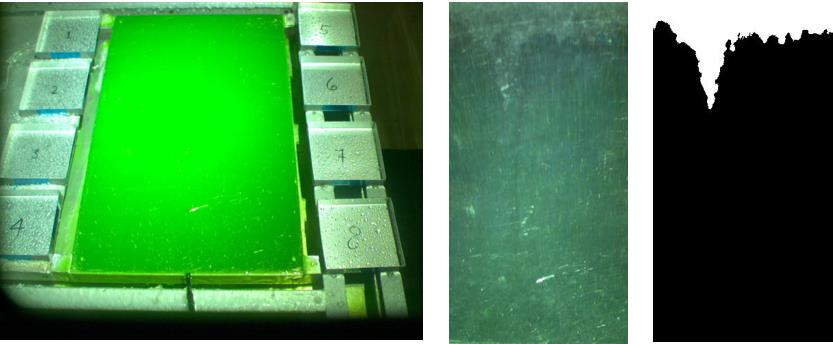
All the endurance tests have in common that the endurance times have to be determined visually by a technician. The failure criterion depends only on the technician’s visual inspection of the plate, since it requires identifying frozen contaminants and mentally calculating the proportion of the test plate that they occupy. This visual inspection has been selected following the actual practice in the industry that after the deicing the aircraft should be inspected visually and manually to ensure that frozen contaminants are completely removed. However, this assessment is subjective and depends on several factors. All of these factors could introduce variability in the endurance time determined by the same person who would repeat the test several times. In addition, different people might determine different endurance times for the same trial. Similarly, the need for permanent supervision makes the procedure tedious since the test can last up to 12 h.

Extended research has been performed by Transport Canada and Federal Aviation Administration to detect the ice and frost deposition on aircraft surface to support the ground operations using remote on-ground ice detection systems (ROGIDS) [7,8]. ROGIDS principally uses near-infrared multi-spectrum detection systems to identify different phases (liquid or solid), like ice and water, over aircraft surface and validate when the ice is removed [9]. Numerous ground-based ice detections systems (GIDS) have been developed and tested over the past years. It may help to detect the ice formation during the precipitation; however, it does not give the percentage of coverage.

This paper proposed help-decision computer-assisted automated methods to determine the endurance time by image analysis, with the goal of minimizing human error resulting from visual inspection and helping in the interpretation of fluid failure.

2. Background

The principal concepts and techniques of image processing used in this work are briefly presented below [10]. Most of them have been used for different applications such as quality insurance image analysis tools in different industries.

2.1. Image Representation

Generally, an image is modeled as positive physical scalar quantity represented as a function f (x, y) in spatial coordinates. In practice, image is composed of a discrete set of elements arranged in a matrix of dimensions N rows per M columns. Each element of the matrix is a pixel with a scalar quantity to represent the color information (binary, gray, or color).

2.2. Histograms Processing

The histograms are spatial domain processing techniques for image enhancement. The histograms are simple to calculate and are used to give an approximate representation of the distribution occurrence of the color level [10].

Studying the histogram of an image makes it possible to visualize the different ranges of colors present on an image to characterize the different objects. Thus, it is sometimes possible to identify a clear separation between the colors of the objects to be identified and the rest of the image.

For images in this proposed work, the frosted pixels would have a range of values different from that of the plate pixels. It would then be possible to use the histogram to segment the image in order to help in detecting the frosted part of the plate.

2.3. Correction Gamma

Correction gamma or power-law transformations is a nonlinear operation defined by the following expression [10]:

$${\mathit{I}}_{\mathit{i}\mathit{j}}^{\prime }=\mathit{\alpha }{\mathit{I}}_{\mathit{i}\mathit{j}}^{\mathit{\gamma }}$$

where I’ and I are respectively the values of a pixel, before and after processing and $\mathit{\alpha }$ and $\mathit{\gamma }$ are constants. With γ < 1, the transformation is compressive and produces clearer images and conversely when γ > 1 the transformation is expansive and produce darker image. So, the correction gamma law is mainly used in image processing for contrast enhancements.

2.4. Otsu Method

Based on a normalized histogram of the image, Otsu’s method iteratively searches an appropriate threshold by minimizing intra-class variance to separate the pixels into two classes, 0 and 1. As an application, Otsu’s method is applied to separate movie images into two classes, foreground scene and background scene [11].

2.5. Spatial Filtering

Linear filtering is a convolution operation between the input signal and the filter’s impulse response. It is used for many purposes in the signal and the image processing applications. Filter impulse response of a discrete image transformation is simply a small matrix, so-called kernel filter. Depending on the values of the kernel filter, a wide range of effects can be obtained as blurring, sharpening, edge detection, etc.

Therefore, a kernel filter W_kl of dimensions (2a + 1) × (2b + 1) and a gray gradient image represented by the matrix I_ij. The element I’_ij of the image matrix modified by this kernel is given by:

$$I_{ij}^{\prime }={\displaystyle \sum _{k=-a}^a\sum _{l=-b}^b}{W}_{kl}^{}{I}_{i-kj-l}^{}$$

this operation is computed for each special location (i, j) by moving the kernel so as to traverse all these sub-matrices in images.

2.6. Laplacian Filter Approximation

The rapid variation of a color can be used to identify the edges between the different areas of an image. This information is used in image processing to detect and to identify objects sharing same features. First and second order differential operators are often used to identify sets of pixels around which there is a discontinuity [12].

As an example, the numerical modelling for the Laplacian filter ${\nabla }_{}^{2}f\left(x,y\right)=\frac{\partial f^2}{\partial x^2}+\frac{\partial f^2}{\partial y^2}$ can be deduced by approximating the differential derivatives as a finite difference of the first-order. Initially, the partial first-order derivative in the x-direction is approximate as:

$$\frac{\partial f^{}}{\partial x^{}}=f\left(x,y\right)-f\left(x-1,y\right)$$

Similarly, the partial first-order derivative in the y-direction is approximate as:

$$\frac{\partial f^{}}{\partial y^{}}=f\left(x,y\right)-f\left(x,y-1\right)$$

The same approximation is applied for the partial second-order derivative respectively in each direction as:

$$\frac{\partial f^2}{\partial x^2}=\frac{\partial }{\partial x^{}}\left(\frac{\partial f^{}}{\partial x^{}}\right)=f\left(x+1,y\right)+f\left(x-1,y\right)-2f\left(x,y\right)$$

$$\frac{\partial f^2}{\partial y^2}=f\left(x,y+1\right)+f\left(x,y-1\right)-2f\left(x,y\right)$$

Therefore, the approximation of Laplacian filter formulation is obtained by summing the partial second-order derivative in x-direction and y-direction:

$${\nabla }_{}^{2}f\left(x,y\right)=f\left(x+1,y\right)+f\left(x-1,y\right)-4f\left(x,y\right)+f\left(x+1,y\right)+f\left(x-1,y\right)$$

Finally, the filter mask used to implement the digital Laplacian is defined by coefficients of ${\nabla }_{}^{2}f\left(x,y\right)$, as follows:

$$\mathrm{kernel}\mathrm{of}\mathrm{Laplacian}=\left[\begin{array}{ccc}0& 1& 0\\ 1& -4& 1\\ 0& 1& 0\end{array}\right]$$

2.7. Gaussian Filter

A Gaussian filter is a linear filter usually used to blur the image, to reduce noise, or to enhance contrast. The symmetrical and centered function of the Gaussian filter with a standard deviation $\sigma$, is defining as follows:

$$G\left(x,y\right)=\frac{1}{2\pi {\sigma }^2}{e}^{-\frac{x^2+y^2}{2{\sigma }^2}}$$

by fixing σ, an appropriate quantification of the spatial function G (x, y) allows us to deduce the coefficients of the Gaussian filter.

2.8. Canny Filter

The Canny filter [13] is a multi-step algorithm used widely to detect a wide range of edges in images. Canny filter is known to perform well for the identification of edges and borders. Basically, Canny filter applies a Gaussian filter followed by a gradient operator and some techniques to remove spurious points on the edges.

2.9. Kalman Filter

In recent progress [14], Kalman filter was proposed essentially to remove the impulse noise in color images were the linear filter performs poorly. According to the authors, the proposed method outperforms other filtering methods.

2.10. Homomorphic Filtering

In the last decade, the homomorphic filtering has been widely used in speech processing to deconvolve the response of the vocal tract and the source excitation of the glottis. By analogy, in its physical aspect the image I (x, y) may be characterized by the product of two components illumination i (x, y) and reflectance r (x, y):

$$f\left(x,y\right)=i\left(x,y\right)\ast r\left(x,y\right)$$

$$0<i\left(x,y\right)<\infty$$

$$0<r\left(x,y\right)<1$$

Homomorphic filtering deconvolves the illumination i (x, y) and reflectance r (x, y) by applying the nonlinear operator log as follows:

$$\log \left(f\left(x,y\right)\right)=\log \left(i\left(x,y\right)\right)+\log \left(r\left(x,y\right)\right)$$

Then, applying Fourier’s transformation $ℱ$ the components become additive and may be separated in frequency:

$$ℱ(\log \left(f\left(x,y\right)\right)=ℱ\left(\log \left(i\left(x,y\right)\right)\right)+ℱ\left(\log \left(r\left(x,y\right)\right)\right)$$

Next, by applying low-pass or high-pass filter, the image can have different transformations according to the applications requirements and needs, among others to make the illumination more even by increasing high-frequency components.

Finally, returning frequency domain back to the spatial domain is performed by using inverse Fourier transform [15].

3. Methodology

In order to develop and evaluate the algorithms, three different endurance tests have been used: Water spray endurance test (WSET), light freezing rain endurance test (LZR), and indoor snow test (SNW). The accumulation setups used for the three tests are presented on Figure 1.

3.1. Endurance Tests

The first test used was the WSET, with its accumulation setup presented on Figure 1A. This test was performed according to the Aerospace Standard AS5901 [6], and reproduced a freezing fog over a cold surface [16]. In a cold room, controlled at a temperature of −5.0 ± 0.5 °C, 22 µm droplets were pulverized from a hydraulic spray system over a refrigerated test support, inclined at an angle of 10°, also at −5 °C. The test support was separated in six sections, that allows for the testing of a fluid in three different positions and measured the icing intensity on the three others. The targeted icing intensity was 5 g/dm²·h. This test was a pass/fail tests that every anti-icing and de-icing fluids used by aircraft pass. The failure time was called visually by an experimented technician when an ice front reaches lines positioned at 25 mm from the top and at 5 mm on each side.

The second test used was LZR as presented in the Aerospace Recommended Practice ARP 5485 [4]. The precipitation was simulated in a 9 m height cold room controlled at a temperature of −3.0 ± 0.5 °C, using 1000 µm water drops that arise from the upper section of the cold room [17]. The test support, presented on Figure 1B, consists of a 30 cm per 50 cm aluminum plate inclined at an angle of 10°, surrounded by eight catching pans to measure accurately the icing intensity. For those particular tests, the targeted intensity was 25 g/dm²·h. In this case the failure time was evaluated visually by an experienced technician and was called when ice covered more than 30% of the plate. The ice front usually started from the top of the plate, but did not occur evenly so the technician needed to transpose some parts to evaluate the accurate time.

The third test used was the SNW, as also presented in the Aerospace Recommended Practice ARP 5485 [4]. The apparatus used was an automated snow deposition device developed by the Anti-icing Materials International Laboratory (AMIL). The apparatus was presented on Figure 1C. It used artificial snow obtained from demineralized water in a cold room maintained at −20 °C. The artificial snow was then stored in a cool box prior being used in the machine. The snow machine positioned in a cold room, controlled at temperatures ranging from 0 to −25 °C. The test plate consists of a 30 cm per 50 cm aluminum plate, controlled in temperature, inclined at an angle of 10°. The intensity was controlled by the scale placed under the test plate. In that case the failure was called when the plate was covered with 30% of white snow that was not absorbed by the fluid.

Along with the three presented setups, the selected cold rooms had been equipped with a visual camera Basler (acA1300-200 uc, Basler Ahrensburg, Germany) equipped with an 8 mm Kowa lens (Kowa, Torrance, Ca). The camera was connected via usb3 ports to a computer where a home-made software saved a picture every 20s. The pictures were taken in color at a 1280 by 1024 pixels format. If required, a light source was installed in the cold room. The camera was positioned in order to obtain the most orthogonal pictures as possible, always from the same position.

3.2. Detection Algorithms

The tool was developed using the software MATLAB (R2017C) (https://www.mathworks.com). Using several available libraries [13,14], the collected images are treated in order to determine the percentage of the area frozen. The main libraries used consist of: The Ōtsu algorithm [18] and Gaussian, Canny [13], Kalman [14], and homomorphic [15] filters. The algorithm was adapted for the three types of precipitations which are presented in the flowcharts of Figure 2.

3.2.1. WSET Detection Algorithm

The WSET algorithm flowchart is presented on of Figure 2A. At the beginning, the test plate was unfrozen and its surface was smooth. A new image of the plate was fed to the algorithm every 20 s. Normally, the freezing fog started to form at the top and/or on the side of the plate. The frozen region was texturized while the surface of the plate remained smooth. The picture before the treatment is presented on Figure 3A. In the selected figure we can see that an ice front was formed on the top of the upper section of the plate and slightly on the right side.

The image was pretreated to enhance edge detection and reduce environmental noise. The first step consisted of a gamma adjustment (γ = 2) (Figure 3B) to put in evidence the ice versus the fluid, which looks darker. The photo was then converted from RGB to grayscale (Figure 3C). A Kalman filter with a gain of 0.7 is then applied to the picture (Figure 3D) to reduce the noise for a sequence of images by predicting the next image. The filter outputs a weighted blend of the actual image and the predicted one in which precipitations falling on the plate was removed. Its efficiency increased with the number of iterations.

Then, edge detection using the Canny algorithm (Figure 3E) detects the highly texturized area in which there was a lot of edges compared to regions which were not frozen. Newly detected edges were accumulated in a matrix representing the state (frozen/not frozen) of the plate at that time (Figure 3F). Then, holes were filled to eliminate gaps between edges (Figure 3G). Since ice forms from the top and/or side of the plate in a continuous way, only the largest connected region was kept (Figure 3H). The failure criterion was then verified (Figure 3I): If the largest connected region touched or passed the redline then the failure was reached, if not compute the next image.

3.2.2. LZR Detection Algorithm

The LZR detection algorithm is based on the principle of background subtraction and is presented of the flowchart of Figure 2B. In this type of precipitation, the ice usually forms from the top of the plate. The initial image, without treatment is presented on Figure 4A.

The image was pretreated to reduce noise and to uniformize lighting by applying a Gaussian filter (std 2) (Figure 4B) and a homomorphic filter (Figure 4C) (gain = 2, cutoff frequency = 0.5, and order of the Butterworth filter = 2).

Then, the background was estimated as follows (Figure 4D). The first background (${\mathit{B}}_1$) was the first image (${\mathit{I}}_1$): ${\mathit{B}}_1={\mathit{I}}_1$. The nth background (${\mathit{B}}_n$) was a weighted blend of the nth image (${\mathit{I}}_n$) and the n − 1 background (${\mathit{B}}_{n-1}$):

$${\mathit{B}}_n=\left(1-\alpha \right){\mathit{I}}_n+\alpha {\mathit{B}}_{n-1}$$

Empirical evidence suggests $\alpha =0.8$ was a good choice for this parameter.

The difference (${\mathit{D}}_n$) between the image and the background was then obtained (Figure 4E). Each new image produces an estimate of where the ice was located. A time-weighted average of these estimations is calculated giving increased importance to the pixels interpreted as different from the background for several consecutive images (Figure 4F):

$${\mathit{D}}_n=\beta {\mathit{D}}_{n-1}+\eta {\mathit{D}}_n$$

empirical evidence suggests $\beta =1.5$ and $\eta =0.2$ are good choices for these parameters.

When the value of a pixel of this average exceeds the predetermined threshold, it was declared frozen pixels. Pixels identified as ice were accumulated over time in a frozen/non-frozen binarized image (${\mathit{F}}_n$):

$$F_{n_{ij}}\{\begin{array}{c}0if{B}_{n_{ij}}<T\\ 1if{B}_{n_{ij}}\ge T\end{array}$$

empirical evidence suggests $T=0.45$ is a good choice for this parameter.

Then, various morphological operations were applied to correct the imperfections of the detected area: Binarization of the image (Figure 4G), filling holes (Figure 4H), and largest connected areas (Figure 4I). Finally, the failure criterion was evaluated, using Figure 4I, from the ratio of frozen areas calculated using the binarized image. If 30% of the image was covered with ice (white pixels), the failure was called. If not, the program used the algorithm from the beginning with the next image.

3.2.3. Snow Detection Algorithm

The snow detection algorithm worked with the principle of color segmentation and was presented on the flowchart of Figure 2C. In that particular case the failure call occurs when 30% of white snow was accumulated. The algorithm should not consider the snow that was falling, neither the snow that was absorbed by the fluid. Figure 5A shows the original picture of a snow test. Some parts of the snow were dissolved in the green fluids and some parts, at the top, were white. The first step of the algorithm consisted in applying a Kalman filter to reduce noise as explained previously (Figure 5B). The grayscale image is binarized using a threshold which will keep only the white snow. A black pixel corresponded to a number of 0 in the gray scale, while a white pixel corresponded to 255 on the same scale. It was determined experimentally that, using a threshold of 220 will keep only the white snow. The obtained binarized image is shown on the Figure 5C. The detected pixels were then added to the previous image (Figure 5D) and the failure criteria was verified: If 30% of the plate was covered with white snow, stop the computation, if not, analyze the next image.

4. Results and Discussion

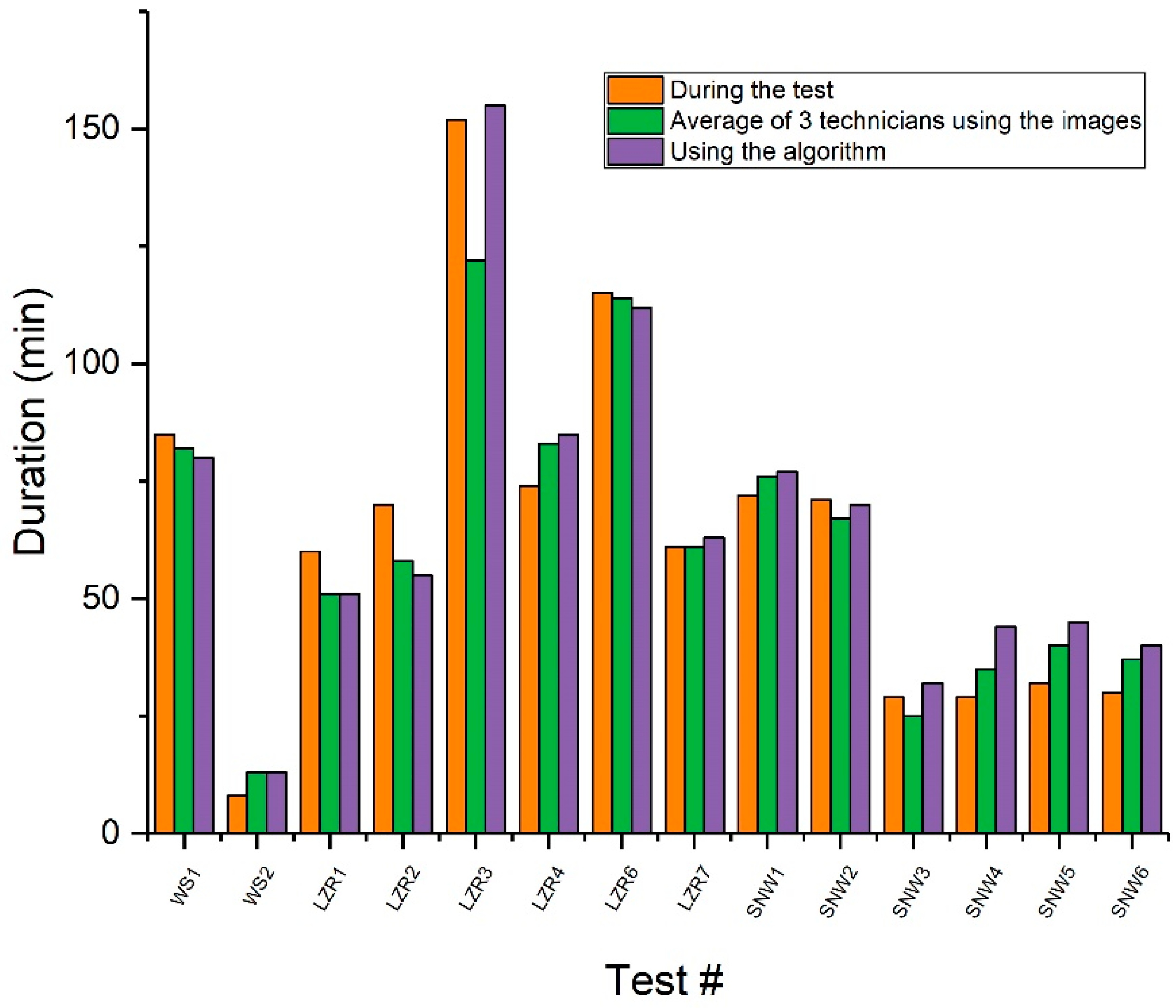
In order to validate the algorithms presented in the previous sections, 14 different tests have been performed and recorded in the three conditions: 2 WSET, 6 LZR, and 6 SNW. The duration times obtained by the algorithms have been compared to two different duration determinations: By the technicians during the test and by the average of three technicians using the same images as the algorithms. The results are presented in

Table 1. Comparison of the algorithms with the test duration determined by the technicians.

Test #	During the Test	Average of 3 Technicians Using the Images	Using the Algorithm	Correlation with During the Test (≤5%)	Correlation with Average of 3 Technicians Using the Images (with S.D. or ≤5%)
	min	min	min	Y/N	Y/N
WS1	85	82 ± 11	80	N	Y
WS2	8	13 ± 1	13	N	Y
LZR1	60	51 ± 1	51	N	Y
LZR2	70	58 ± 2	55	N	Y
LZR3	152	122 ± 1	155 *	Y	N
LZR4	74	83 ± 2	85 *	N	Y
LZR6	115	114 ± 0	112	Y	Y
LZR7	61	61 ± 10	63	Y	Y
SNW1	72	76 ± 4	77	N	Y
SNW2	71	67 ± 1	70	Y	Y
SNW3	29	25 ± 3	32	N	N
SNW4	29	35 ± 5	44 *	N	N
SNW5	32	40 ± 5	45	N	Y
SNW6	30	37 ± 6	40	N	Y

* Test has been stopped before the algorithm can call the failure.

and in Figure 6. Two different limits have been selected, the first using the standard deviation and if the standard deviation was too low, an arbitrary limit of 5% of difference has been selected for the comparison.

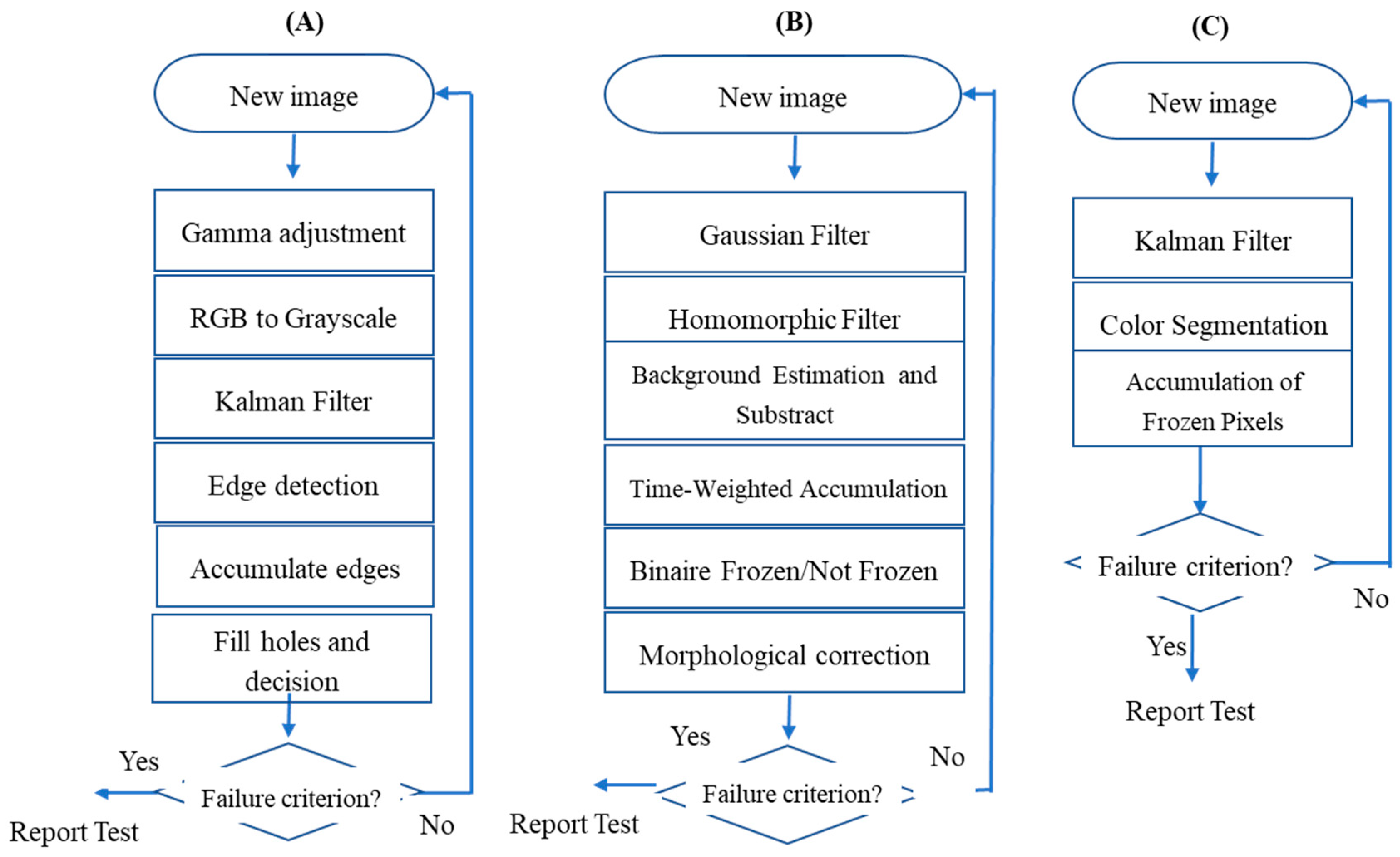
The first two tests compared are the WS1 and the WS2. When comparing the time determined by the algorithm and by the average of three technicians using the images, there was non-significant difference. However, the algorithm does not determine the same duration as the one determined during the tests, giving time 63% higher than the technicians in the case of WS2.

The second algorithm developed, for LZR, has been tested in six different tests: LZR1, LZR2, LZR3, LZR4, LZR6, and LZR7. In two cases, the algorithm does not meet the failure criterium, so the time of the last image has been considered the failure duration. In the case of the LZR004, the ice front covered 29%, slightly under the failure criteria. When the deviation standard is considered, there is no significant difference between the algorithm and the duration determined by the three technicians using the images for only two tests: LZR1 and LZR7. By applying the second criteria, the algorithm remains valid for LZR2, LZR4, and LZR6. The results brought by the algorithm are more significant for this type of test. It is also interesting to see that the algorithm fits with the duration determined during the tests for two tests LZR6 and LZR7; but has a considerably higher percentage difference.

The third algorithm developed for the indoor snow test has been tested under six different tests: SNW1, SNW2, SNW3, SNW4, SNW5, and SNW6. In one case, SNW4, the algorithm does not meet the failure criterium, so the time of the last image has been considered the failure duration. In the case of the SNW4, the white snow covered 29%, slightly under the failure criteria. When the standard deviation is considered, there is no significant difference between the algorithm and the duration determined by the three technicians using the images for only three tests: SNW1, SNW5, and SNW6. By applying the second criteria, the SNW2 test also fits with both the algorithm and the average of the technicians. However, the percentage difference is too high for two tests: SNW4 and SNW5. By comparing the time determined during the test only the SNW2 meets the algorithm.

From the results presented, it is clear that the algorithms meet the average duration determined by the technician using the images: The duration fit in 11 tests out of 14, so 79% of success. However, the algorithms do not fit with the duration determined during the tests: 3 tests fit out of 14, only 20% of success.

The most important cause of error is the reflection of light on the test plate. When these reflections are static, a homomorphic filter has helped to significantly reduce this problem. However, in the case of snow tests, the device for dispersing snow moves over the test plate while reflecting light. These reflections are very intense and white and change their position constantly. Not only must the algorithm not detect these reflections as white snow it tries to detect, but they also make a significant part of the plate inaccessible for a time since completely white. This cause of error is probably responsible for the fact that the only two failures in determining the endurance time of the algorithm compared to the technicians who used the photos are snow tests.

Another cause of error arises from the use of the Kalman filter. It is necessary to filter the images because of precipitation falling on the plate that should not be detected as ice. The Kalman filter is particularly effective in eliminating these sudden noises. However, an undesirable consequence of its use is when ice front progresses rapidly. During the first moments of this progression, the filter interprets sudden change as noise. The algorithm then takes a little more time before the quickly appearing iced part is detected and computed.

There is also a significant difference between the endurance time determined by the technician present during the test and that determined by the technicians using the images. In fact, in order to determine whether the images allow a correct interpretation of reality, it would be relevant to verify during the test if, for the same technician, the visual inspection of the plate gives the same endurance time as with the images. On the one hand, the camera is closer to the test plate than the technician present, which could facilitate the detection of ice. On the other hand, the images contain artifacts that could interfere with the detection of ice and thus give the advantage to the technician present during the test.

Without doing more research, it is difficult to know which of the endurance times, between the determined one, in presence by a single technician, and the one determined with the images by three technicians, is the closest to reality. However, it can be seen that the algorithms give results equivalent to the human for most of the tests if only the images are used. So, if there is a difference between the determined endurance times in relation to those determined with the images is explained by a problem with them, it is possible to believe that by improving their quality, the developed algorithms would help to determine endurance times equivalent to those of technicians present during the tests.

In addition, the results show that, in general, using the same images, different technicians determine different endurance times. For example, a 21-min difference in endurance time is observed for test WS1. These discrepancies are to be expected since, on the one hand, the visual evaluation of the frosted parts is subjective and, on the other hand, the zone of failure (for WSET) or the percentage of iced areas (for LZR and SNW) must be mentally valued by the technicians.

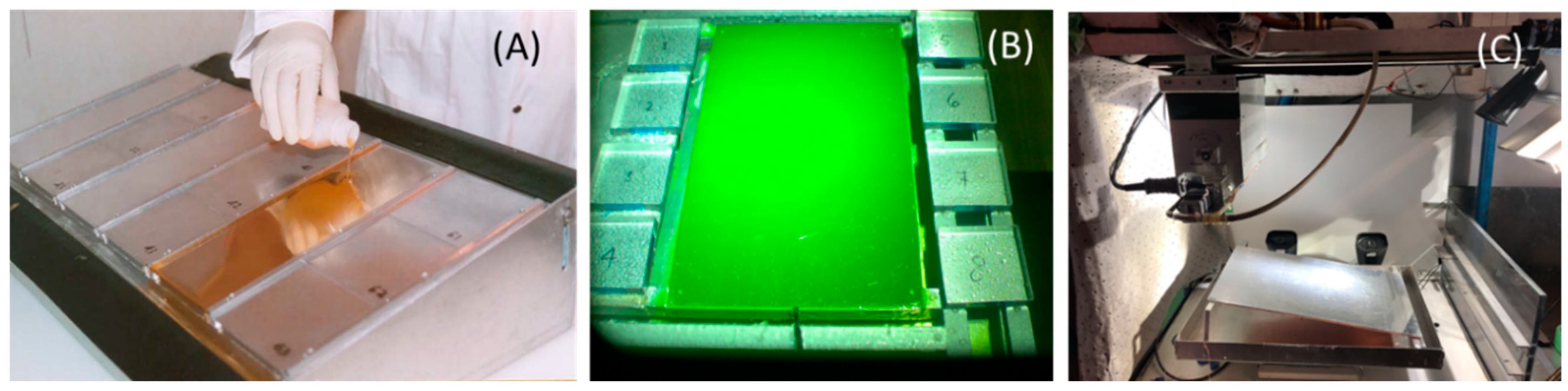
What limits the automated determination of endurance time is significantly the ability to obtain good quality images. First, the camera placed in the climate chamber is exposed to precipitation, which randomly obstructs the lens. In addition, the camera should be placed far enough from the plate as to not interfere with the test and cannot be orthogonal to the test due to the experimental setup. Moreover, the results obtained show a significant difference between the endurance times obtained by a technician present during the tests and those obtained by technicians who used the images of these tests. It will be necessary to determine if this difference is caused by the quality of the photos and, if it is the case, to improve the quality of these until finding the same endurance time in the presence as with the images.

Also, the experimental data used for the verification of the algorithms are the same as those used for their elaboration. Although the endurance times were not known beforehand, it would be relevant to validate the endurance times obtained by these algorithms using other experimental data. Indeed, it should be verified that the algorithms give results comparable to those of a human for other tests for which the experimental conditions vary (light, cameras, fluid, etc.) in order to verify that the parameters are not over-adjusted. Even though, the purpose of the algorithms is to determine the endurance time, it would be relevant to verify that they identify the same iced parts on the test plate as the technicians. Indeed, in this research work, the performance of algorithms for the detection of frost has not been evaluated. To do this, each technician could identify the areas he considers iced on the image of the moment of failure. Subsequently, images summarizing all the photos of the technicians would be created. These would be divided into three classes of areas: The areas they all consider as iced, the areas they all consider as un-iced and the areas that some consider iced and others not at the time of failure.

In order to evaluate the performance of the algorithms proposed for automated ice detection, the areas considered iced by the technicians would be compared to the iced/non-iced binary images produced by the algorithm. The percentage of ice detected by the software and by at least one of the technicians would be calculated. Then, the percentage of ice not detected by the software but identified by all the technicians would be given. Finally, the percentage of false positives, that is to say ice detected by the software but by none of the technicians would be presented. This method would verify that the algorithms give valid endurance times because they detect the frost correctly.

5. Conclusions

Three algorithms to determine the endurance time of anti-icing fluids by image analysis were developed for different types of tests based on image analysis using MATLAB.

In order to develop these algorithms and evaluate the validity of their results, the different tests have been carried out using prescribed experimental setup.

The endurance times obtained by the algorithms were compared with the endurance times determined by the technician present during the tests. Of the 14 trials for which the images could be used, the endurance time determined by the algorithms was only valid for 3 of them, i.e., there was a difference of less than 5% between the endurance time determined by the technician present and that produced by the MATLAB program.

In addition, a group of three technicians determined the endurance times of these tests from their photos. The averages of these endurance times and their standard deviation were calculated. The endurance times obtained by the algorithms were then compared with these average values. Of the 14 trials for which the images could be used, the endurance time found by the algorithms was valid for 11 of them, that is, whether it was within a standard deviation of the average technician, or there was a difference of less than 5% between them.

The developed algorithms could be improved and used as a helping tool for a technician to ensure to call the failure properly.

References

1. Leroux, J. Guide to Aircraft Ground Deicing; SAE G-12 Steering Group, Ed.; SAE International: Warrendale, PA, USA, 2017; p. 134. [Google Scholar]
2. SAE International. AMS 1424 Deicing/Anti-icing Fluid, Aircraft, SAE Type I; Society of Automotive Engineers: Warrendale, PA, USA, 2012. [Google Scholar]
3. SAE International. AMS 1428 Fluid Aircraft Deicing/Anti-Icing, Non Newtonian (Pseudoplastic), SAE Types II, Type III and Type IV; Society of Automotive Engineers: Warrendale, PA, USA, 2016. [Google Scholar]
4. SAE International. ARP5485B: Endurance Time Test Procedures for SAE Type II/III/IV Aircraft Deicing/Anti-Icing Fluids; Society of Automotive Engineering: Warrendale, PA, USA, 2017. [Google Scholar]
5. SAE International. AS5900 Standard Test Method for Aerodynamic Acceptance of SAE AMS1424 and SAE AMS1428 Aircraft Deicing/Anti-icing Fluids; Society of Automotive Engineers: Warrendale, PA, USA, 2016; p. 28. [Google Scholar]
6. SAE International. AS5901D Water Spray and High Humidity Endurance Test Methods for SAE AMS1424 and SAE AMS1428 Aircraft Deicing/Anti-icing Fluids; Society of Automotive Engineers: Warrendale, PA, USA, 2019; p. 13. [Google Scholar]
7. APS Aviation Inc. Feasibility of ROGIDS Test Conditions Stipulated in SAE Draft Standard AS5681; APS Aviation Inc.: Laurent, QC, Canada, 2007; p. 212. [Google Scholar]
8. SAE International. AS5681B Minimum Operational Performance Specification for Remote On-Ground Ice Detection Systems; Society of Automotive Engineers: Warrendale, PA, USA, 2016. [Google Scholar]
9. Zhuge, J.-C.; Yu, Z.-J.; Gao, J.-S.; Zheng, D.-C. Influence of colour coatings on aircraft surface ice detection based on multi-wavelength imaging. Optoelectron. Lett. 2016, 12, 144–147. [Google Scholar] [CrossRef]
10. Gonzalez, R.; Woods, R. Digital Image Processing; Pearson Prentice Hall: Upper Saddle River, NJ, USA, 2008; Volume 1. [Google Scholar]
11. Otsu, N. A threshold selection method from gray-level histograms. IEEE Trans. Syst. Man Cybern. 1979, 9, 62–66. [Google Scholar] [CrossRef] [Green Version]
12. Solomon, C.; Breckon, T. Fundamentals of Digital Image Processing: A Practical Approach with Examples in Matlab; John Wiley & Sons: Hoboken, NJ, USA, 2011. [Google Scholar]
13. Canny, J. A computational approach to edge detection. IEEE Trans. Pattern Anal. Mach. Intell. 1986, 6, 679–698. [Google Scholar] [CrossRef]
14. Kavitha, L.S.M.C. Kalman Filtering Technique for Video Denoising Method. Int. J. Comput. Appl. 2012, 975, 8887. [Google Scholar]
15. Pitas, I.; Venetsanopoulos, A.N. Nonlinear Digital Filters: Principles and Applications; Springer Science & Business Media: Berlin, Germany, 2013; Volume 84. [Google Scholar]
16. Villeneuve, E.; Brassard, J.-D.; Volat, C. Effect of Various Surface Coatings on De-Icing/Anti-Icing Fluids Aerodynamic and Endurance Time Performances. Aerospace 2019, 6, 114. [Google Scholar] [CrossRef] [Green Version]
17. Brassard, J.-D.; Laforte, C.; Volat, C. Type IV Anti-Icing Fluid Subjected to Light Freezing Rain: Visual and Thermal Analysis; SAE Technical Paper: Warrendale, PA, USA, 2019. [Google Scholar]
18. Agrawal, P.; Shriwastava, S.; Limaye, S. MATLAB implementation of image segmentation algorithms. In Proceedings of the 2010 3rd International Conference on Computer Science and Information Technology, Chengdu, China, 9–11 July 2010; pp. 427–431. [Google Scholar]
Figure 1. Endurance time tests: (A) water spray endurance test (WSET) refrigerated support, (B) LZR support plates, and (C) Anti-icing Materials International Laboratory (AMIL’s) indoor snow machine.
Aerospace 07 00039 g001
Figure 2. Flowcharts of the algorithms developed: (A) WSET, (B) LZR, and (C) indoor snow test (SNW).
Aerospace 07 00039 g002
Figure 3. WSET detection algorithm for WSET (A) original image, (B) gamma adjustment, (C) grayscale RGB conversion, (D) Kalman filter, (E) contours detection with algorithm of canny, (F) addition with what has been previously detected, (G) fill holes, (H) largest connected region, and (I) representation of the failure zone.
Aerospace 07 00039 g003
Figure 4. Algorithm of ice detection under light freezing rain: (A) original image, (B) Gaussian filter, (C) Homomorphic filter, (D) background, (E) difference between the image and the background, (F) addition with which has been detected previously, (G) binarization, (H) fill the holes, and (I) largest connected region.
Aerospace 07 00039 g004
Figure 5. Algorithm of snow detection (A) original image of an indoor snow test, (B) image after Kalman filter, (C) binary image, and (D) cumulative image.
Aerospace 07 00039 g005
Figure 6. Comparison of the algorithms with the duration determined by the technicians during the test and using the same photos as the algorithms.
Aerospace 07 00039 g006