Aeroelastic Wing Planform Design Optimization of a Flutter UAV Demonstrator

Abstract

In this work, a study to design a highly flexible flutter demonstrator for the development and testing of active flutter suppression is presented. Based on the UAV mission, a bi-objective design optimization problem can be formulated. The aeroelastic UAV characteristic and imposed constraints, defined by operational aspects and the structural integrity are described by surrogate modeling. Within the framework of the multi-criteria optimization, an approach to construct the equally spaced Pareto frontier with a new approach for non-convex problems is presented. An efficient Pareto configuration to meet a natural low speed and low frequency is identified and its main influencing design features are analyzed.

1. Motivation of Flexible Wing Technologies

Improving aircraft technologies with respect to performance and costs is a constant challenge for aerospace researchers. Nowadays, environmental friendliness plays an increasingly important role in structural and aerodynamic design optimizations [1]. In order to improve aerodynamics by reducing induced drag, a clear trend towards wings with a higher aspect ratio (AR) is being pursued. As shown in the work of Kenway and Kennedy, aircraft configurations with lower fuel consumption can thus be achieved [2,3]. These more slender wings in combination with highly lightweight structural designs result in wing structures with considerably greater elasticity compared to currently comparable aircraft structures. This trend can be seen, for example in the B787 or A350 aircraft. If future aircraft will be able to benefit from an further increase, solutions to control the wing deformation and vibration have to be developed.

Promising technologies under investigation can be characterized in active and passive stabilization mechanisms. In the passive solutions, efforts are made to achieve directional wing stiffness in order to specifically influence wing properties such as load paths and vibration behavior. This can be realized with orthotropic materials as presented in [4]. It is shown, that with the additional design degrees, improved solutions for aircraft wings in terms of load elevation are possible. A further approach is to achieve an anisotropic distribution of stiffness through the systematic arrangement of structural components or topology, as presented in [5]. In addition, active methods using control devices to control the wing exist. Typical examples are active load alleviation systems in which several trailing edge control surfaces of the wing are used to reduce the loads, e.g., caused by gusts [6].

Both methods are extensively investigated in various programs, such as the EU-funded project Smart Fixed Wing Aircraft or the NASA Fixed Wing program. The reduction of the internal wing loads, so that airframe structures can be dimensioned smaller to save weight, are aims to be pursued with both active control and passive structure technologies. In order to finally evaluate active technologies, additional aspects such as failure probability or additional system weight must be taken into account. An overview of the development of active methods, including its benefits and strengths compared to passive alleviation is given in [7].

Aeroelastic Problem Description

The certification authorities request that wings are flutter-free within their operating envelope [8]. Traditionally, aircraft are designed to avoid flutter under normal flight conditions and also ensure an adequate safety margin from the flutter boundary. This is normally achieved in a passive manner by adjusting the stiffness and mass distribution in the structural design as required. This approach has the disadvantage that it cannot adapt to changing flight conditions, such as those resulting from fuel consumption. In addition, the structural stiffening of the more flexible wings leads to an increase in structural mass, which is directly related to higher fuel consumption. The use of active flutter suppression techniques could possibly lead to an extension of the flight envelope without any additional reinforcement of structures, thus increasing fuel efficiency and performance.

As a consequence of certification, active stabilization methods for civil aircraft have to be developed and tested. When wings are operated closer or in their aeroelastically unstable condition, their behaviour must be well understood. This also includes the applied models for the representation of the relevant physics with sufficient accuracy. In order to verify the developed simulation tools and models, as well as the active control technologies, real flight tests and demonstrations are necessary. High development costs, the possible loss of the aircraft and personal injury are significant risks for medium-sized to full scale aircraft. Projects such as the X-56A [9] and FLEXOP [10] attempt to investigate technologies such as flutter suppression, wing stabilization capabilities or active load reduction for wings with higher aspect ratio based on demonstrators for unmanned aerial vehicles (UAV). The development of UAVs to investigate the described challenges is one possible approach to minimise these risks.

A predefined, unstable aeroelastic condition is one of the main interests of a flutter UAV demonstrator. Since the phenomenon of wing flutter is in focus, the aerostructural wing design and sizing are essential. Operational aspects of the FLEXOP UAV, as described in [11], impose additional constraints on the design. The flight path with visual line of sight restriction can be highlighted as one of the most important effects in the design of such UAVs, as it limits the maximum flight speed. Configurations with the lowest possible flutter speed and the required structural integrity to ensure safe operation are therefore preferred. As the cost and complexity of the UAV system increases with aircraft size, small systems are the preferred choice. The Huginn [12] or MUTT [13] UAV demonstrators are examples for low frequency body freedom flutter demonstration platforms. In comparison, the FLEXOP demonstrator follows the idea of investigating classical wing flutter.

The design parameters influencing the aeroelastic behaviour are stiffness and mass distribution as well as the aerodynamic forces defined by the wing planform and aerofoil. In addition to the intended flutter instability, the UAV demonstrator must fulfill a standard flight mission outside the unstable flight regime. From this, a complex design task can be concluded with opposing design goals.

In the following work, it is analyzed how the wing planform of such a demonstrator should be selected. The basic design of the wing structure, except for the dimensioning of the individual parts with static load conditions, remains unchanged in this investigation. Surrogate modeling to make the simulation computationally tractable and the problem formulation as a multi-optimization task, that includes a method for solving a non-convex equally spaced Pareto frontier, is used to identify possible UAV configurations.

2. Parametric Elastic Aircraft Model

The wing planform is the focus of the study and is performed on an elastic aircraft configuration. The starting configuration for this work is the demonstrator developed in the Flexop project including its flight mission and boundary conditions as presented in [10,11]. The UAV configuration has a span of 7 (m) and a MTOW of 65 (kg). The wing-fuselage arrangement is designed as a high wing aircraft with V-tail and is equipped with a jet engine. From the mission planning, the design flutter speed was specified to be $50 \mathrm{m}{\mathrm{s}}^{-1}$. The specified target flutter speed is the determined maximum speed at which the aircraft can be safely operated within the permissible flight pattern. Lower speeds would improve the operation of the demonstrator and are therefore preferred. Therefore the trade-off between wing planform and stiffness shall be investigated in the present work to favor lower flutter speeds.

Due to the coupled flight mechanics, a change in the wing planform also influences flight stability and dynamics of the aircraft’s rigid body motion. Since the flutter behavior is coupled with the rigid body dynamics, especially with more elastic wings, it is necessary to include this effect in the investigation, so that different configurations can be compared with each other. To achieve the same flight characteristics for each configuration the tail volume $V_T$ is adjusted accordingly. The applied aircraft design approach is summarized in Figure 1. Based on the six design parameters, wing area $S_W$, aspect ratio $AR$, taper ratio $TR$, wing sweep $\Lambda$ and the two laminate thicknesses $t_{CFRP}$ and $t_{GFRP}$, different wing layouts are created with a wing empennage/fuselage model adapted for each configuration. With the respective aircraft configurations, the properties required for the evaluation are then calculated and incorporated into a surrogate model. On last the optimization, the problem is finally solved.

The system requirements and details of the parametric aircraft design process are described in the following chapters.

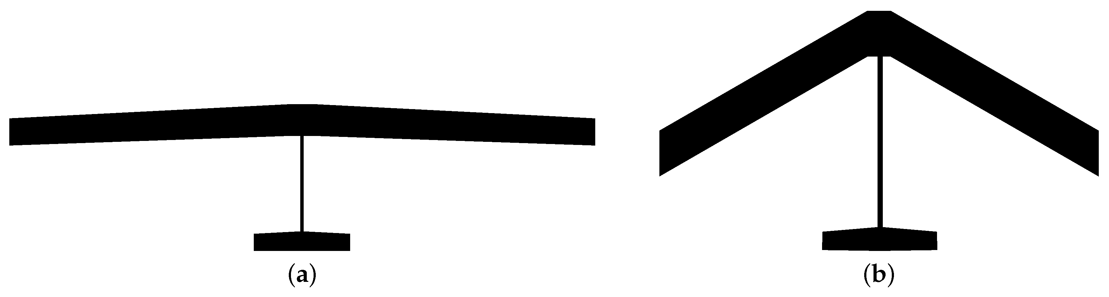
2.1. Wing Planform Parameter and Structural Design

A parametric model of the wing and its internal structure is used to investigate several different wing planforms. The wing is defined with the parameters wing area $S_W$, AR, TR and $\Lambda$. The wing area $S_W$ is used to see the influence of the size scaling of the UAV configuration. The influence of different lift distribution is covered by the aspect and taper ratio. The wing sweep $\Lambda$ is used to study different bending-torsional coupling effects.

All four wing planform design parameters are indirectly influencing the structural layout and hence the wing stiffness. A larger aircraft generates more lift and therefore the structural components have to be dimensioned stronger. The same holds for the lift distribution, when it gets shifted more outwards, as it is the case with a rising aspect and taper ratios. Bending-torsion coupling tends to support a low flutter speed, but with higher sweep angles the torsional loading also increases, which is why the wing also has to be reinforced. In order to investigate these trade-offs, the adaptation of the structural sizing is also necessary.

The inner wing structure consists of a front spar, rear spar, ribs and is designed together with the wing shell in composite design. The highly stressed spars and ribs near the root consist of monolithic carbon fiber reinforced polymer (CFRP) with a Young’s modulus of $E=138\mathrm{GPa}$ in the fiber direction. Special considerations are necessary for the design of the wing shell. The construction of a flutter wing at very low airspeeds requires a tailor-made adjustment of the stiffness and naturally leads to a problem of material scalability. Due to the composite construction, the adaptation of the stiffness is restricted by:

• Ply Count: usually limited to a minimum number for production reasons.
• Ply thickness: limited by layers with a minimum thickness available on the market ($t_{min}\approx 0.05\mathrm{mm}$)

Both restrictions have the effect that the stiffness of the wing shell cannot be reduced arbitrarily, even if other constructive constraints are not violated. The shell in the present study is made from a glas fiber reinforced polymer (GFRP) foam core sandwich, with the following advantages:

• The GFRP plies have a Young’s modulus in the fiber direction of $E=27.4\mathrm{GPa}$, and are therefore less stiff than CFRP.
• Thin plies are prone to buckling. The foam core sandwich design increases bending stiffness significantly (parallel axis theorem) with a moderate growth in structural mass compared to a full monolithic design.

The structural components is shown in Figure 2. The composite layup of the spars is chosen to maximize the bending stiffness while the wing shell is used to adjust the torsional stiffness. The wing shell is accordingly symmetrically designed with $\pm 45deg$ layup. The wing shell has the same structure over the entire span, except at the wing root. In order to carry the high loads and to ensure a clean load transfer for the sandwich, the foam core is successively replaced by a monolithic design. To support the bending loads, front and rear spar are built up with $64\%$$0deg$ and $36\%$$\pm 45deg$ plies. The zero degree direction for spars and shell is determined by the sweep angle $\Lambda$. Since the highest loads occur at the wing root, the layup is thickest here and is reduced by $20\%$ along the span over three steps. To achieve the necessary integrity for different wing planforms, the thickness of the individual plies is scaled accordingly. Therefore the thickness parameters $t_{CFRP}$ (mm) and thickness $t_{GFRP}$ (mm) are used to control the bending and torsional stiffness. With the presented structural design it is assumed that bending and torsion loads are carried separately via spar and shell. With increasing wing sweep, this approach is only possible to a limited extent, since typically torsion and bending are beared by both structural components. In addition, it is assumed that plies of any thickness are available. To avoid a discontinuous optimization task, the ply thickness is continuously adjusted between 0.01 and 2.0 (mm). For the conceptual design task this is considered justified and has to be converted to a discrete layup in the later detailed design. The remaining ribs are not included in the sizing process and therefore remain constant. For the evaluation of the structure integrity, only spar and the wing shell is used.

The Finite Element Method (FEM), as implemented in MSC NASTRAN, is used to investigate the flexible wing characteristics such as structural deformation, integrity and stability. The flutter solutions are calculated using the pk-method as provided by NASTRAN. The first 15 elastic eigenmodes of the free-flying aircraft are used to represent its dynamics. To model the composite layup, shell elements as shown in Figure 2, in combination with the classical laminate theory is used as stiffness modeling approach. To investigate several different configurations, a parametric geometry model was implemented and passed to the FE pre-processor for meshing. In pre-processing, the system masses are modelled using lumped masses, boundary conditions are defined and the aerodynamic interface is created. Fuselage and empennage are treated as rigid body, so that no structural dimensioning is necessary. Elastic wing, rigid fuselage, empannage are connected by rigid body elements in the aircraft’s center of gravity.

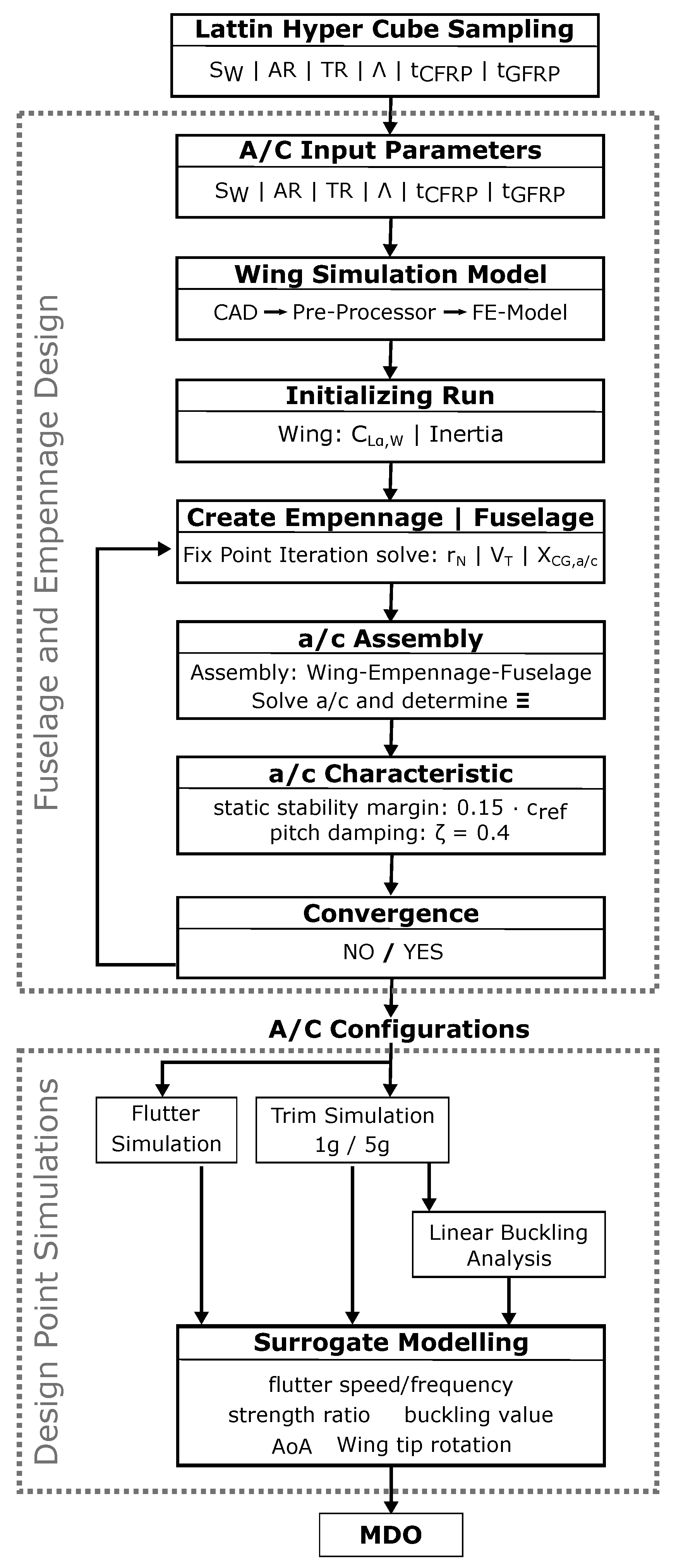
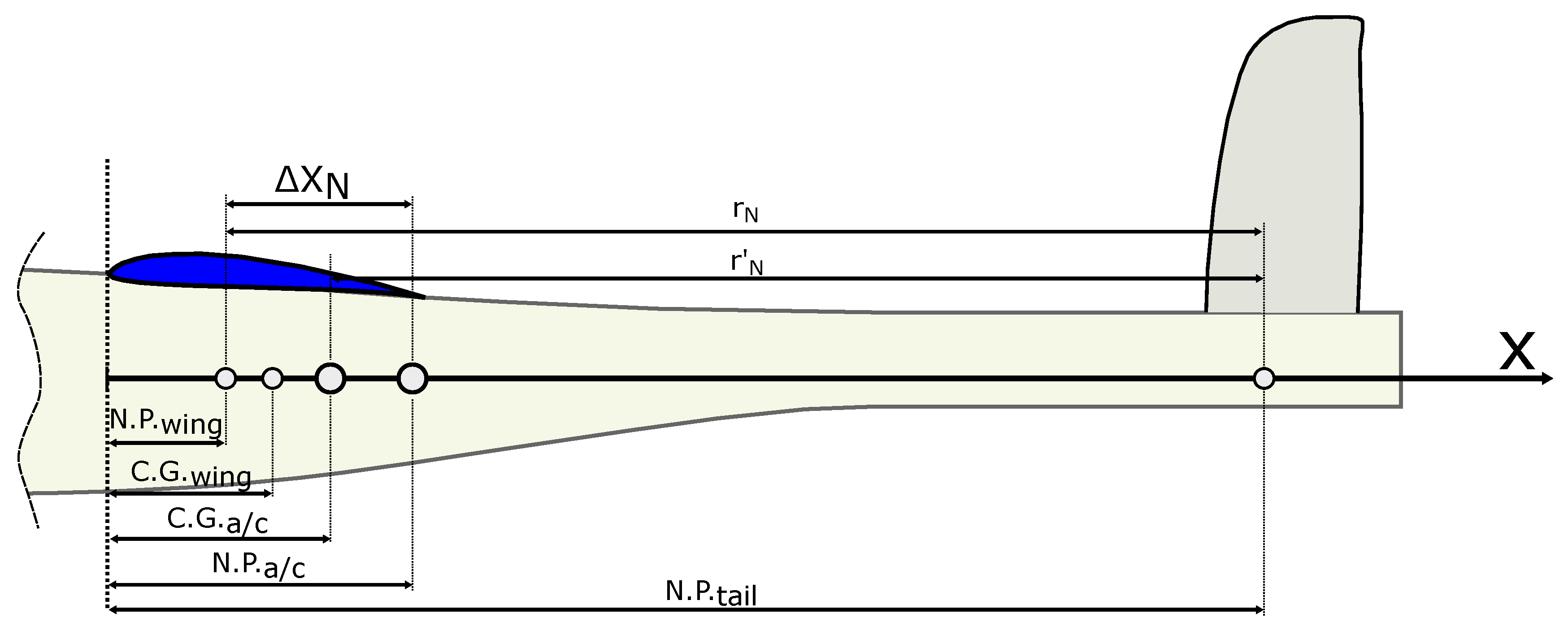
2.2. Parametric Empennage and Fuselage Design Process

The rigid body dynamics of the entire aircraft cannot be neglected for reasonable investigations on flexible wings. Therefore, the flexible wing model is extended by a rigid fuselage and a tail to a complete aircraft model. Different wing planforms require different centers of gravity (C.G.) and neutral point (N.P.) positions for a stable configuration. Therefore, the empennage and sub-components are arranged in such a way that the natural static and dynamic flight stability of the aircraft is the same in every configuration.

Before the actual investigations begin, an aircraft pre-design loop is carried out. Based on the wing plan form, the aircraft tail and fuselage are designed in such a way that each configuration fulfils the following characteristics.:

• Static flight stability margin ${\epsilon =N.P.}_{a/c}-{C.G.}_{a/c}=0.15·c_{ref}$;
• Relative pitch Damping $\zeta =-\frac{\sigma }{2·{\omega }_0}=0.4$.

Both criteria are based on experience with UAVs flown by hand and are therefore rather conservative. In case the dynamic behaviour is supported by a flight controller or the UAV is completely controlled by an autopilot, the corresponding constraints have to be reassessed. In order to meet these requirements, the position of the neutral point and center of gravity as well as the size of the empennage cannot be selected independently of each other. The used reference point definitions are presented in Figure 3, with the aircraft reference coordinate system located at the wing leading edge.

As the wings Neutral Point ${N.P.}_{wing}$ and Center of Gravity ${C.G.}_{wing}$ are defined by the wing planform, the remaining design variables are

• $r_N$: lever arm of the tail.
• $V_T$: Empennage Volume, defined as $V_T=r_N·S_T$, where $S_T$ the empennage reference area is.
• $X_{C.G.}$: Center of Gravity full aircraft.

These three size parameters are non-linearly dependent on each other, and in order to find a solution so that the static and dynamic flight stability conditions are fulfilled, the computational fixed-point iteration method is used for solving. Because there is more than one mathematical solution, the additional constraint that forces the tail volume $V_T$ to create a minimal wetted surface area is added. This restricts the solution space and separates mathematically correct but physically unreasonable designs from meaningful ones. The approach, in which the fuselage wetted surface is approximated by a truncated cone depending on $r_N$ is, e.g., presented in Gudmundsson [14].

The empennage design is defined as a V-Tail configuration and has for all configurations the same form parameters. Therefore, the only remaining design variable is the size. With the tail surface $S_T$ and the leverage $r_{N.P.}$, the aircraft neutral point $X_{N.P.,a/c}$ is calculated from Equation (1) as shown in Schlichting [15].

$$X_{N.P.,a/c}=X_{N.P.,w}+\frac{A_r·C_{L\alpha ,T}·ϵ·\frac{q_h}{q}}{C_{L\alpha ,W}+A_r·C_{L\alpha ,T}·ϵ·\frac{q_h}{q}}$$

(1)

The aerodynamic derivative $C_{L\alpha ,W}$ as well as $X_{N.P.,W}$ of the wing is calculated in a previous initialization run. For this case, the wing is clamped and an aerodynamic model based on the vortex-lattice-methode (VLM), as implemented in NASTRAN [16], is used.

The Area Ratio parameter in Equation (1) is defined as $A_r=\frac{S_T}{S_{Ref}}$. The down-wash parameter $ϵ$ as well as the dynamic pressure correction $\frac{q_h}{q}$ are two remaining parameters to determine. Schlichting [15] gives some estimations of those correction terms, which are based on an elliptical lift distribution on an unswept wing. Schlichting [15] further differentiates between a single furled and unfurled wing vortex layer, which interacts with the empennage. These assumptions and unknown correction parameters cause significant deviations in the final aircraft configuration, especially for higher swept wings. The two correction parameters are therefore combined to one empennage correction factor $\mathsf{\Xi }$, which is identified by a computational aerodynamic evaluation via the VLM of the combined wing-empennage configuration.

To evaluate the relative pitch damping of the aircraft configuration, the absolute damping factor $\sigma$ and the natural frequency ${\omega }_0$ is calculated according to Equations (2) and (3).

$$\sigma =\frac{\frac{1}{2}·q·S_{ref}·C_{ref}^2}{2·U_{ref}·I_{yy}}·C_{mq}$$

(2)

$${\omega }_0=\sqrt{\frac{q·S_{ref}·C_{ref}·C_{m\alpha }}{I_{yy}}}$$

(3)

The aerodynamic derivatives $C_{m\alpha }$ and $C_{mq}$ are approximated, according to Schlichting [15], with the wing and tail lift slope derivatives $C_{L\alpha ,W}$, $C_{L\alpha ,T}$ and the introduced correction term $\mathsf{\Xi }$.

$$C_{m\alpha }=\frac{X_{NP,a/c}-X_{c.g.}}{C_{ref}}·(C_{L\alpha ,W}+A_r·C_{L\alpha ,T}·\mathsf{\Xi })$$

(4)

$$C_{mq}=2·C_{L\alpha ,W}·{\left(\frac{X_{NP,W}-X_{c.g.}}{C_{ref}}\right)}^2+2·C_{L\alpha ,T}·A_r·\mathsf{\Xi }·{r_N^{{}^{\prime }}}^2$$

(5)

To evaluate the dynamic behaviour of the aircraft configuration, an inertia model for Equations (2) and (3) as well as for the FE model is required. The inertia data of the wing are directly derived from the FE model. The empennage mass is modeled by taking the existing FLEXOP tail unit as reference value and scaling it with the reference surface $m_{tail}=m_{tail,ref}(\mathrm{kg}/{\mathrm{m}}^2)·S_t$. The empennage is further treated as a point mass, so the inertia contribution can be described simply by $I_{yy,tail}=m_{tail}·{r_N^{{}^{\prime }}}^2$.

The fuselage inertia is assembled by discrete mass points of the subcomponents such as batteries, receiver, flight control devices and their relative position. The internal component arrangement is assumed to be equal for each configuration and is based on the FLEXOP arrangement. The tail boom is the only component taken into account that depends on the size. The cross-section of the tail boom is considered constant and is scaled accordingly with the length $r_N^{{}^{\prime }}$. The fuselage mass is thus calculated $m_{fuselage}=m_{fuselage,FLEXOP}+m_{tailboomsection}\left(\mathrm{kg}/\mathrm{m}\right)·(r_N^{{}^{\prime }}-r_{N,FLEXOP}^{{}^{\prime }})$. The total mass model is obtained by adding up the three main components and can be specified as follows.

$$\begin{array}{cc}\hfill m& =m_{wing}+m_{tail}+m_{fuselage}\hfill \\ \hfill I_{yy}& =I_{yy,wing}+m_{tail}·{r_N^{{}^{\prime }}}^2+I_{yy,fuselage}+m_{tailboomsection}\left(\mathrm{kg}/\mathrm{m}\right)·\frac{(r_N^{{}^{\prime }}-r_{N,FLEXOP}^{{}^{\prime }})·r_N^{{}^{\prime }}}{4}\hfill \end{array}$$

(6)

3. Mathematical Optimization Statement and Surrogate Modeling

Specifically, when UAV operation is limited to the visual line of sight, as is the case with [10] and is described in detail by [11], the possible flight trajectory is limited. This is why, from an operational point of view, the first configuration goal is to achieve a low flutter speed. Reducing the flutter speed as much as possible expands the possible test path and shortens the required acceleration distances.

For the analyzed demonstrator, active flutter suppression is achieved by active control of the outer control surface. A successful control design, such as that presented in [17], requires that the flap actuation speed is fast enough to provide sufficient bandwidth. In practice, this leads to the problem that when designing a demonstrator, most of the available servo drives do not satisfy the required speed. The second goal of the demonstrator configuration is therefore to achieve the lowest possible flutter frequency of the first unstable flutter mode.

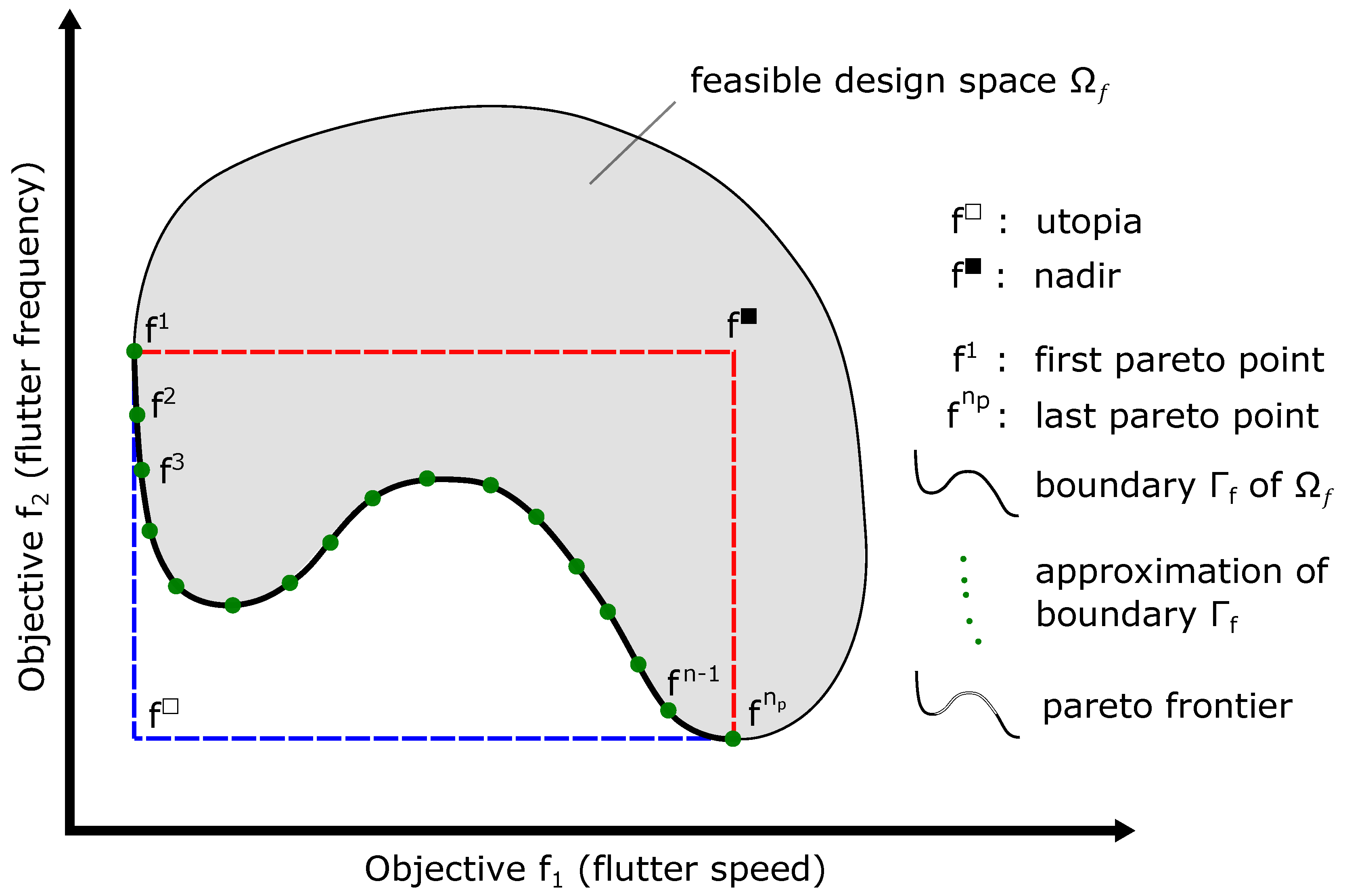
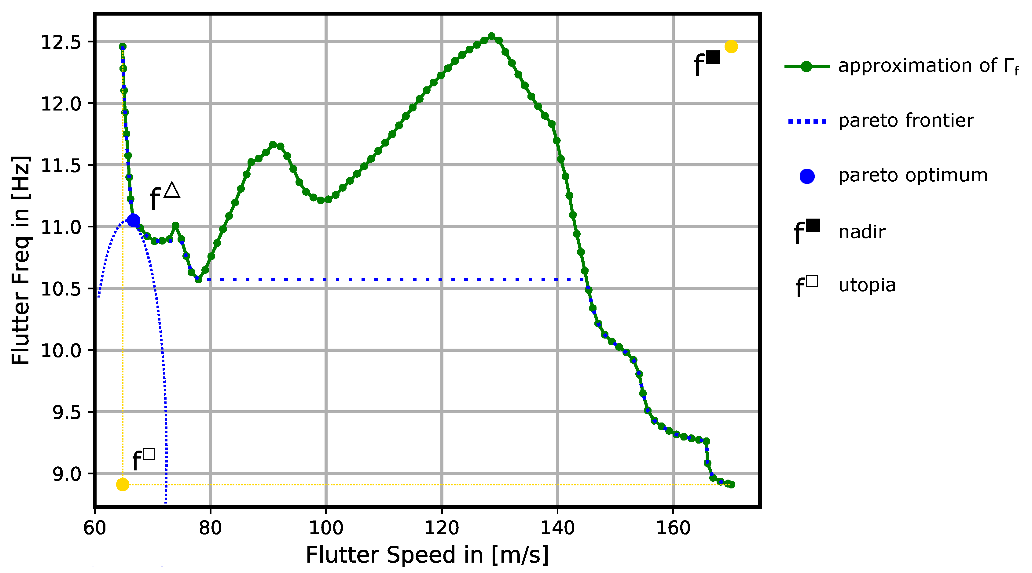
3.1. Multi-Objective Optimization Technique

For the optimization task the idea, as presented in Pereyra [18] or Schatz [19], to solve the Pareto frontier by equidistant points, is resumed. Both solve the bi-objective problem by scalarizing the two design goals $f_1\left(x\right)$ and $f_2\left(x\right)$ to a single objective optimization problem. In the case of the scalarized bi-objective optimization, the objective function can be defined as Equation (7), with $\lambda$ as an independent optimization variable.

$$\begin{array}{cc}\hfill \underset{x,\lambda }{\mathrm{minimize}}& f=\lambda ·f_1+(1-\lambda )·f_{2}0\le \lambda \le 1\end{array}$$

(7)

The central idea of an approximation of the Pareto boundary by equally discrete points $f_{opt}^n$ is represented in Figure 4. All values of the feasible criteria define the feasible design space ${\Omega }_f:=f\left(x\right):g\left(x\right)>=0,x\in \chi$ as illustrated in Figure 4. The values of the fictitious criteria are indicated by $f^{\blacksquare }$ for nadir and $f^{\square }$ for utopia. In addition, one finds the Pareto frontier on the boundary ${\Gamma }_f$ of ${\Omega }_f$. The approximation is started at $f_{opt}^1$ and developed towards $f_{opt}^n$. The Pareto frontier is suspended between the start and end points, called anchor points.

It is shown, that the approach works well on convex optimization problems. In fact, it is observed that the approach for non-convex Pareto boundaries is only partially stable, e.g., for piecewise convex parts.

Once the frontier reaches a curvature reversal point, by switching off one of the single objectives through setting $\lambda =0$ or $\lambda =1$, the scalarization approach starts evolving back to the starting anchor point. Mishra [20] gives a good overview about non-convex problems and different approaches to resolve the Pareto front. The scalarization approach is also discussed as only conditionally applicable. For the presented work, the approach after Pereyra [18] is extended by the idea of an arc-length method. The optimization task is therefore formulated as

$$\begin{array}{cc}\hfill \underset{x}{\mathrm{minimize}}& F(f_1,f_2)\hfill \\ \hfill \mathrm{subject}\mathrm{to}& g\left(\mathbf{x}\right)\ge 0\hfill \\ \hfill & g_{BS}\left(\mathbf{x}\right)\ge 0\hfill \\ \hfill & g_{AS}\left(\mathbf{x}\right)\ge 0\hfill \\ \hfill \mathrm{and}& h_{\gamma }\left(\mathbf{x}\right)={\gamma }^2\hfill \\ \hfill \mathrm{with}& \mathbf{x}\in \chi \hfill \end{array}$$

(8)

with x being the vector of design variables, F defining the objective and $\mathbf{g}\left(\mathbf{x}\right)$ the inequality, respectively $\mathbf{h}\left(\mathbf{x}\right)$ the equality constraints. As given in Equation (8) and illustrated in Figure 5, three additional side constraints must be fulfilled after Equation (9).

$$\begin{array}{cc}\hfill g_{BS}\left(x\right)& =\parallel (f^{n+1}-f^n)(f^n-f^{n-1})\parallel \ge 0\hfill \\ \hfill g_{AS}\left(x\right)& =\parallel (f^{n+1}-f^n)(f^n-f^{n_p})\parallel \ge 0\hfill \\ \hfill h_{\gamma }\left(x\right)& =\parallel f^{n+1}-f^n{\parallel }^2={\gamma }^2\hfill \end{array}$$

(9)

The first so-called back-step inequality constraint $g_{BS}$ is introduced so that no previously calculated solution is recalculated. As mentioned above, this limitation for non-convex problems is not a guarantee that the algorithm will continuously approach the second anchor point during Pareto front reconstruction. Therefore, the optimization task is extended by the anchor-stepping inequality constraint $g_{AS}$, which enforces to resolve the next Pareto point to the end anchor point. The equality constraint $h_{\gamma }$ ensures, that the distance between the previous Pareto point and the next is equally spaced. The distance between two subsequent solutions is given by

$$\gamma ={\displaystyle \frac{c}{n_p}}·\parallel f^{n_p}-f_1\parallel$$

(10)

With the two anchor points $f^1$ and $f^{n_p}$, the curvature factor c and point size parameter $n_p$, the approximated point resolution of the curve is defined.

The objective function is defined by Equation (11), which corresponds to a minimization of the angle between the vectors $v_1$ and $v_2$. In this case, the start anchor point $f^1$ is the minimum of the single objective $f_1$. For the case, that $f^{n_p}$ is chosen as a starting point, F has to be maximized.

$$\begin{array}{cccc}\hfill & \hfill & \hfill F& ={\displaystyle \frac{v_1\times v_2}{\parallel v_1\times v_2\parallel }}·arccos(v_1·v_2)\hfill \\ \hfill with:& \hfill & \hfill v_1& ={\displaystyle \frac{1}{\parallel f^n-f^{n-1}\parallel }}(f^n-f^{n-1})\hfill \\ \hfill & \hfill & \hfill v_2& ={\displaystyle \frac{1}{\parallel f^{n+1}-f^n\parallel }}(f^{n+1}-f^n)\hfill \end{array}$$

(11)

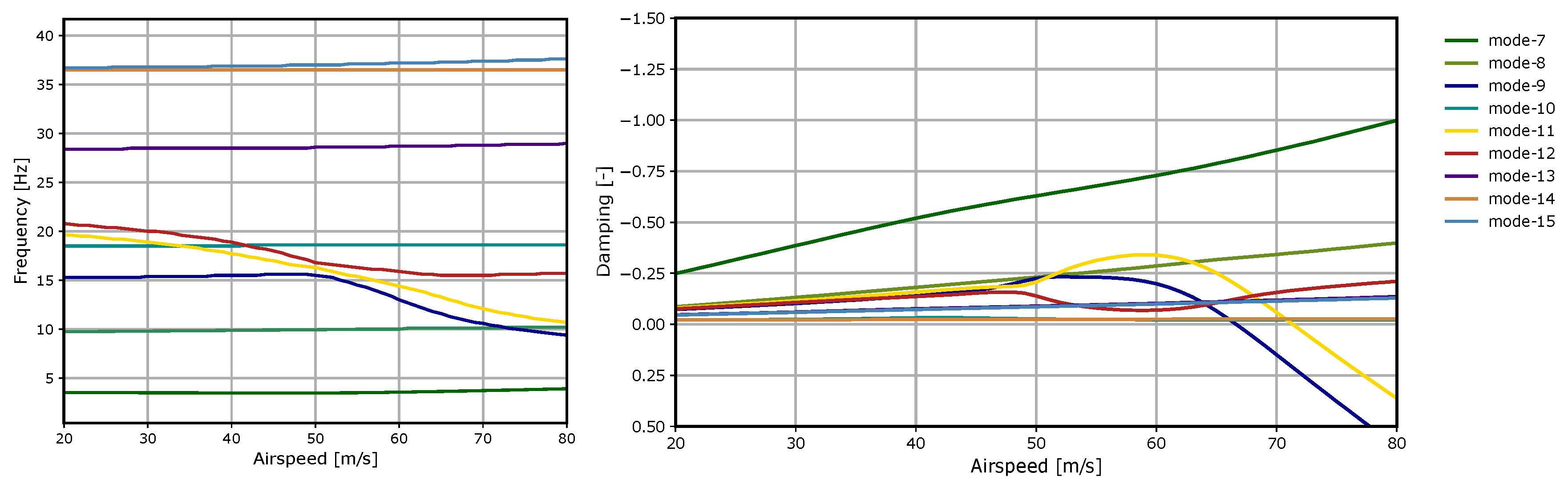
3.2. Aeroelastic Design Optimization

The aeroelastic optimization task is solved with the gradient based SLSQP algorithm [21]. The described design and optimization process is implemented in a design environment based on c++ and python programming language. To ensure, that the results are not a local phenomenon, the optimization runs are started from multiple starting points, where each point is determined by scanning the design space with a latin hypercube sampling plan.

The design objectives for the presented study have already been discussed. To achieve a feasible aircraft configuration, additional technical constraints have to be stated. These are the elasto-stability of the wing shell, structural integrity for a possible 5g load case, a maximum elastic wing tip twist to prevent negative stall and an additional aerodynamic constraint, which ensures that the aircraft generates enough lift at take-off and landing.

To evaluate the structural integrity, the aircraft is brought into a trimmed load case of $n_z=5g$ at $U_{\infty }=50 \mathrm{m}{\mathrm{s}}^{-1}$. Both values are taken from the design boundary conditions of Flexop and were derived from the flight mission planning as presented in [11]. The 5g load case corresponds to a maneuver with bank angle of $65\left(\mathrm{deg}\right)$ with a safety factor of two. In order to demonstrate sufficient safety in manual flight, conservative values are used as appropriate. The composite structural load is evaluated based on the failure theory after Tsai-Wu. The resulting aerodynamic loads are further used for a linear buckling analysis of the wing shell. For the investigation carried out here, a horizontal wing is assumed. To ensure that no negative lift or stall occurs, the maximum elastic wing twist at the tip is limited to $-\Delta 4deg$ at $n_z=5g$. This value was taken as an assumption, based on the lift slope of the used airfoil, for the design study, as many different configurations have to be covered. In the detailed wing design, this condition can be softened with appropriate wing twisting in the jig shape. Especially at higher wing sweeps with a strong bending-torsion-coupling the limitation of the elastic twist is a constraint to filter out too flexible wing configurations.

To make sure, that the wing size is large enough to produce enough lift at lower speeds, an additional constraint of a maximum $AoA\le 8deg$ is set. The defined maximum AoA is already high for a clean wing to guarantee a safe operation in all weather conditions. Based on the knowledge of similar UAVs e.g., [10], the AoA can be significantly lowered, by using the flaps as high lift devices, which is why a maximum AoA of $8deg$ is an eligible assumption.

Summarized, the multi-objective aeroelastic optimization task is defined as

$$\begin{array}{cc}\hfill \underset{x}{\mathrm{minimize}}& F(\frac{U_{flutter}}{U_{ref}},\frac{f_{flutter}}{f_{ref}})\hfill \\ \hfill \mathrm{subject}\mathrm{to}& g_{buckling}\left(\mathbf{x}\right)\ge 1.0\hfill \\ \hfill & g_{strength Ratio}\left(\mathbf{x}\right)\ge 1.0\hfill \\ \hfill & g_{AoA}\left(\mathbf{x}\right)\le 8.0deg\hfill \\ \hfill & g_{twist}\left(\mathbf{x}\right)\ge -4.0deg\hfill \\ \hfill & g_{BS}\left(\mathbf{x}\right)\ge 0\hfill \\ \hfill & g_{AS}\left(\mathbf{x}\right)\ge 0\hfill \\ \hfill \mathrm{and}& h_{\gamma }\left(\mathbf{x}\right)={\gamma }^2\hfill \\ \hfill \mathrm{with}& \mathbf{x}\in \chi \hfill \end{array}$$

(12)

with the flutter speed $U_{flutter}$ defined as the first unstable aeroelastic eigenmode and the corresponding flutter frequency $f_{flutter}$. To normalize the two objectives, the fictive point utopia $[U_{ref},f_{ref}]=f^{\square }$ is used. The lower ${\mathit{x}}^l$ and upper ${\mathit{x}}^u$ boundaries for the six wing design parameters are listed in

Table 1. Design space definition.

x	${\mathit{x}}^{\mathit{l}}$	${\mathit{x}}^{\mathit{u}}$	Unit
S	$2.0$	$4.0$	m${}^2$
AR	$8.0$	$22.0$	−
TR	$0.2$	$1.0$	−
$\Lambda$	$0.0$	$30.0$	deg
$t_{CFRP}$	$0.01$	$0.2$	mm
$t_{GFRP}$	$0.05$	$0.2$	mm

.

3.3. Surrogate Model Construction

The presented technique to resolve the Pareto frontier has the drawback, that many system evaluations of high-fidelity numerical simulations have to be undertaken. That is why a surrogate model is used to decrease the computational effort, by evaluating a limited number of construction points.

In a first step, the design space is scanned by a sampling plan constructed by the latin-hypercube sampling method, as presented in [22,23]. Radial basis functions (RBFs) are used for surrogate modeling because they can represent the response values at the construction points and their accuracy can be further refined with additional support points. Thus, non-linear responses, as they typically occur with mode jumps in the flutter calculation, can more properly be covered. The use of RBFs in combination with a Gaussian base as shown in Equation (13) requires the calculation of the weighting factor ${\theta }_k$, where $X={[x^1,x^2,\dots ,x^m]}^T$ stands for the supporting points. The kriging method, as described in [23], is used for this purpose.

$$\psi (\theta ,x^{\left(i\right)},x^{\left(j\right)})=\prod _{k=1}^{m}exp(-{\theta }_k·{\parallel x_k^{\left(j\right)}-x_k^{\left(i\right)}\parallel }^2)$$

(13)

One of the advantages of surrogate modeling is the possibility to filter out noise. This can be caused by over sampling or by the response behavior of the construction points themselves, if numerical methods with a defined residuum and convergence criteria are used. Forrester [23] showed how regression models can be used to reduce this problem. As presented by Hoerl [24], the regression kriging method is therefore used.

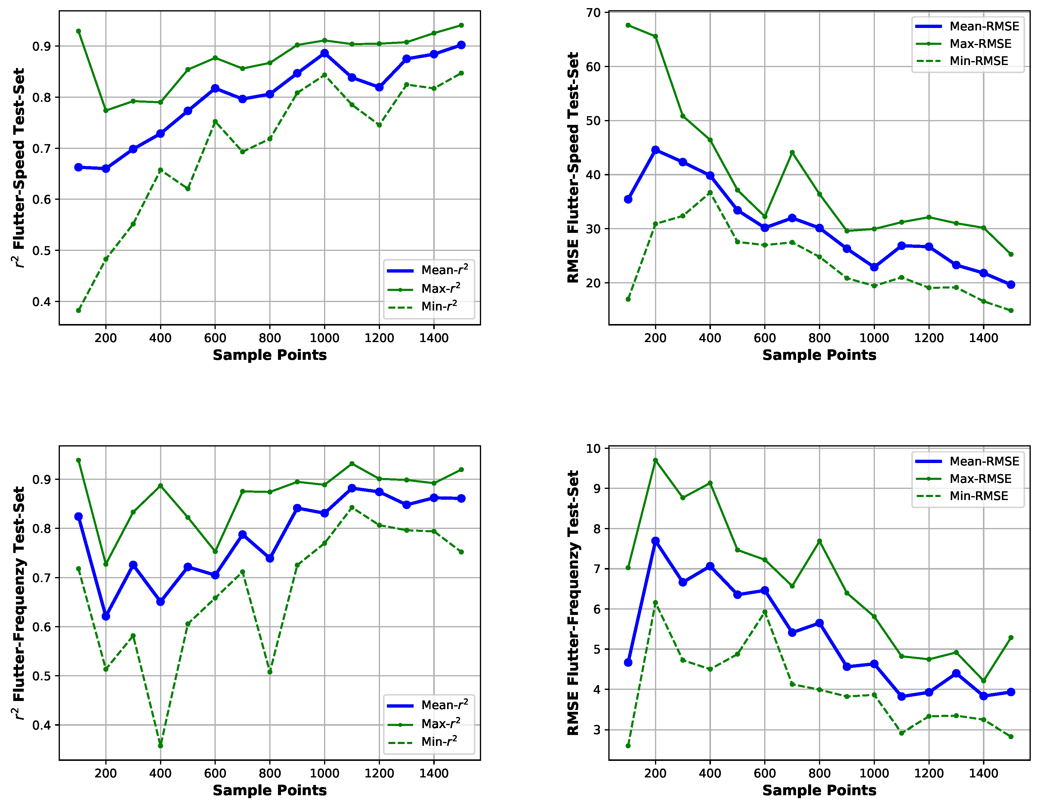
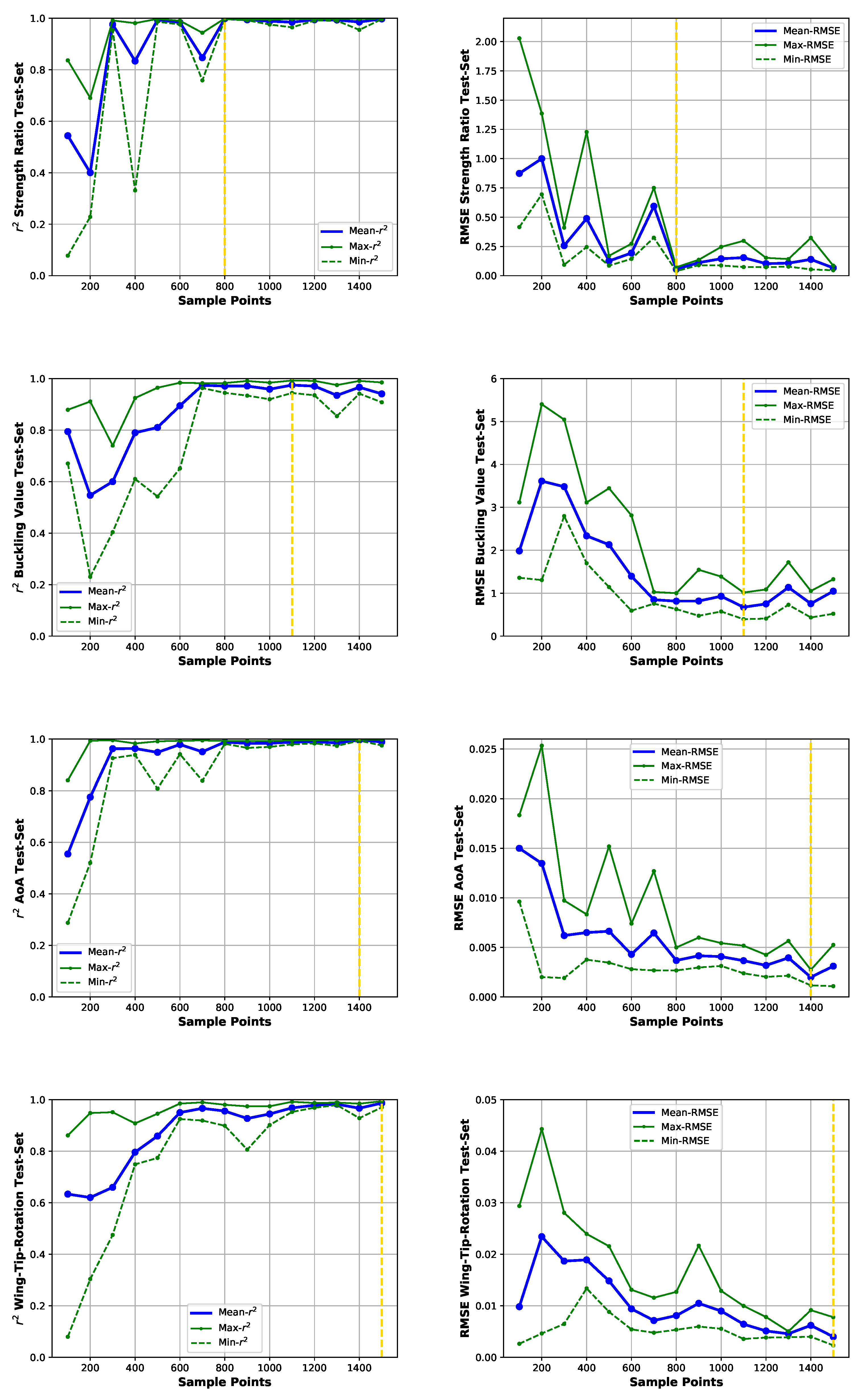
3.4. Surrogate Model Cross-Validation

The surrogate model is started from an initial data set of 500 samples points, designed according to a latin-hypercube sampling plan. Global model accuracy is trained by additional support points that minimize the mean quadratic model error (MSE). For the final model a total of 1500 construction points are available. The k-cross-validation technique is used to estimate how well the surrogate model represents new data points. The construction points are divided into five equal subsets q. Four subsets are used to construct the surrogate model and the remaining fifth set is used for validation. To evaluate the models, the root mean square error (RMSE) according to Equation (14) and correlation coefficient $r^2$ according to Equation (15) of the validation set is applied. Here f stands for the real observation at design point i and $\psi$ for the surrogate model based prediction.

$$RMSE=\sqrt{{\displaystyle \frac{{\sum }_{i=0}^{n_q}{(f^i-{\psi }^i)}^2}{n_q}}}$$

(14)

$$r^2={\left({\displaystyle \frac{cov(f,\psi )}{\sqrt{var\left(f\right)var\left(\psi \right)}}}\right)}^2$$

(15)

The results of RMSE and correlation coefficient for different sampling rates of the objective variables are presented in Figure 6. As validation criterion the correlation coefficient, as suggested by [23], $r^2>0.8$ is used. The RMSE is used as additional validation criterion. As an extra final validation, the RMSE of the final simulated Pareto front set of construction points is used. As this is an iterative approach, it is not possible to use the final results as a validation set during the construction of the surrogate model. Nevertheless, it indicates how well the design area of interest is covered compared to the global accuracy and how reliable the final results are.

The cross-validation results for the two objective function are shown in Figure 6. The correlation criterion is met for the flutter speed objective after 600 design points. Additional design points provide further possibilities for improving accuracy. With the full constructions point set, both correlation criterion and RMSE are performing best. In case of the flutter frequency, the best performing model could be achieved with 1100 construction points.

It should be noted, that the automated parametric aircraft model design process provides all objective variables and constraints in each run. This means that design points, estimated as possible improvement for one surrogate model, do not necessarily lead to any improvement of other surrogate models. In order to keep computing times as short as possible, one should ensure that all available data sets are used. Regardless of the use of the regression kriging method, model overfitting could be identified in some areas, which is why for the flutter frequency, the reduced data set is used.

The correlation factor and RMSE results for the constraint variable are shown in Figure 7. In principal, the same behaviour as in the flutter frequency can be observed, which is why for each constraints, the best performing data set, marked in yellow, is used for the design task.

Table 2. Validation set RMSE and max error results.

	RMSE	Max Absolute Error
flutter speed (m/s)	1.80	5.12
flutter freq (Hz)	0.689	1.412
strenght ratio (-)	0.013	0.028
buckling value (-)	0.098	0.571
AoA $(deg)$	$3.1\times {10}^{-4}$	$1.1\times {10}^{-3}$
Wing-Tip Rotation $(deg)$	$4.0\times {10}^{-4}$	$1.4\times {10}^{-3}$

provides a summary of the RMSE and maximum error results for the six models.

4. Aircraft Conceptual Optimization Result

The surrogate based optimization study begins with the individual problems of obtaining a UAV configuration with a minimum flutter speed and a UAV configuration with a minimum flutter frequency. These optimizations are performed independently of each other, with the side constraints specified in the multi-criteria optimization. The results are listed in

Table 3. Single objective optimization results.

	Flutter Speed	Flutter Frequency
optimization objective flutter speed	$64.8 \mathrm{m}{\mathrm{s}}^{-1}$	$12.4\mathrm{Hz}$
optimization objective flutter frequency	$170.0 \mathrm{m}{\mathrm{s}}^{-1}$	$8.91\mathrm{Hz}$

. The corresponding wing planforms of both configurations are presented in Figure 8, where the conflicting design requirements become clear.

For a low speed flutter demonstrator, the optimization algorithm converges to configurations with the largest possible wing area. The same can be said for the wing aspect ratio. Since wings with higher AR values are naturally more flexible and therefore more sensitive to flutter, this result seems to be reasonable. In the case of wing stiffness, the $t_{CFRP}$ bending dominated design parameter converges to the upper limit, while the $t_{GFRP}$ torsional stiffness tends to converge to the lower limit. The strength ratio constraint for the wing shell is active for the presented configuration. As the torsional stiffness is at the lower design limit, the wings deflection is limited through a high bending stiffness. Furthermore, the torsional load is lowered by reducing the wing sweep.

For the case of a low flutter frequency, much higher operating speeds are required. Compared to the low speed configuration, the optimization tends to converge to higher sweep angles as well as taper ratios close to one. The higher taper ratio and wing sweep results in an increased wing inertia, which benefits low structural eigen frequencies. Due to the higher wing sweep, the torsional loading is significantly increased. As in the low speed configuration, the material strength is the limiting structural constraint. The torsional stiffness parameter thus reaches its upper limit, while the bending stiffness is at a moderate level closer to the lower boundary. The high torsional stiffness of the wing explains, why a flight speed of $170.0 \mathrm{m}{\mathrm{s}}^{-1}$ is required.

Multi-Objective Optimization Results

The multi-objective design approach as described in the previous chapter is used to reconstruct the Pareto-front with the two objective variables flutter speed and frequency. The resulting frontier is plotted in Figure 9. From the Pareto frontier point set, marked in blue, the Pareto point $f^{△}$ is derived. The $f^{△}$ configuration comprisses the best compromise between having a low flutter speed and frequency. The resulting flutter results from the surrogate model as well as verification results, obtained from a simulation, are shown in

Table 4. Flutter results of the Pareto optimal configuration.

	Flutter Speed	Flutter Frequency
surrogate model results	$66.7 \mathrm{m}{\mathrm{s}}^{-1}$	$11.1\mathrm{Hz}$
verification results	$66.0 \mathrm{m}{\mathrm{s}}^{-1}$	$11.4\mathrm{Hz}$

.

The wing planform result of the Pareto optimal configuration is displayed in Figure 10. Compared to the single objective optimizations, the Pareto optimal configuration has close similarities with the low-speed configuration. The wing’s aspect ratio is slightly reduced and the taper ratio increased. The wings stiffness is again characterized by having a maximum bending stiffness and the lowest possible torsional stiffness. The damping over velocity as well as frequency over velocity for the aeroelastic modes are shown in Figure 11. The first six eigenmodes are rigid body modes and not included in the plot. The unstable flutter mode-9 and mode-11 is shown in Figure 12. Both modes show a high contribution of torsional modes, which is due to the low torsional stiffness. This is confirmed by the three natural modes contributing to the flutter mechanism shown in Figure 13. A description of all three configurations is given in

Table 5. Design summary of the three concluding UAV configurations.

	Min Flutter Speed Configuration	Min Flutter Frequency Configuration	Pareto Optimal Configuration
Wing Area $S_W\left({\mathrm{m}}^2\right)$	4.0	3.6	4.0
Aspect Ratio	22.0	9.5	20.1
Taper Ratio	0.84	1.0	0.95
Wing Sweep $\Lambda \left(\mathrm{deg}\right)$	2.2	30.0	3.3
$t_{CFRP}$	0.2	0.02	0.2
$t_{GFRP}$	0.05	0.2	0.05
Total UAV weight $\left(\mathrm{kg}\right)$	64.1	64.2	63.5
Wing Span (m)	9.38	5.848	8.971
Empennage Leaver Arm $r_N\left(\mathrm{m}\right)$	1.972	2.249	1.9801
5g max wing tip $u_z$-deflection (mm)	231.4	172.6	208.1

.

5. Summary and Conclusions

In this work, an approach to investigate the influence of the basic wing planform for a UAV flutter demonstrator with a natural critical flutter frequency at low speed was investigated. A design tool chain based on surrogate modeling techniques, including aeroelastic, structural and flight mechanic characteristics of an UAV is developed. The influence of the wing planform and the structural stiffness dependent on static sizing load cases has been analyzed. Different constraints, which can be derived from operational aspects are used to define a single- and multi-objective optimization task. To evaluate different UAV configurations a reconstruction of the Pareto frontier is undertaken. To resolve the Pareto frontier, a computational construction approach through equidistant Pareto points, applicable for non-convex problems is introduced.

A Pareto efficient configuration, providing low-speed flutter characteristics combined with a low flutter frequency is identified. Since the configurations have to fulfill their actual flight mission besides the intentionally added instability, an arbitrary wing stiffness and therefore low operating speeds is not possible. The torsional stiffness of the wings could be identified as a key factor for a low flutter speed, which is limited by the structural integrity of the wing shell. Consequently, the optimized configurations show wing planforms with lower sweep angles to reduce the additional torsional loading. Lower flutter frequencies could be achieved with higher wing sweeps. The additional torsional loads lead to a considerable thickening of the wing shell and thus to an increase in torsional stiffness and thus to higher flutter speeds.

The present work was carried out with the background of a conceptual UAV design. Further lowering of the flutter speed was not possible, as the wing shell structural integrity would be violated. On a more detailed design level, highly stressed areas such as the wing root can be further strengthened. It is to be expected that by softening the strength constraints further, a further reduction of the flutter speed would be possible without increasing wing masses. The distribution or installation of additional masses is another possibility to influence flutter frequency and speed. This additional possibility is investigated in [25] for the case of classical wing flutter or [26] for body freedom flutter. The disadvantage of distributed masses, especially with small UAVs, are local vibration phenomena, which have only a limited relation to upscaled wings and were therefore not considered in this paper as an additional design variable.

For the preliminary design of a flutter wing the statement can be made that smaller wing sweeps should be preferred, to reduce the additional torsional moment and avoiding strong influences by the static sizing load cases. Larger wings in combination with a higher aspect ratio lead to more flexible wings and also favour the required objectives. A large taper ratio leads to more structural mass in the outer area and additionally reduces the natural frequencies of the bending modes. For a wing with sweep, the same applies to the torsional modes.

References

1. Cheelhaase, J.; Grimme, W.; O’Sullivan, M.; Naegler, T.; Klötzke, M.; Kugler, U.; Scheier, B.; Standfuß, T. Klimaschutz im Verkehrssektor; Aktuelle Beispiele aus der Verkehrsforschung. Wirtschaftsdienst 2018, 98, 655–663. [Google Scholar] [CrossRef] [Green Version]
2. Kenway, G.K.; Martins, J.R. Multipoint High-Fidelity Aerostructural Optimization of a Trasport Aircraft Configuration. J. Aircr. 2014, 51, 144–160. [Google Scholar] [CrossRef] [Green Version]
3. Martins, J.; Kennedy, G.; Kenway, G.K. High Aspect Ratio Wing Design: Optimal Aerostructural Tradeoffs for the Next Generation of Materials. In Proceedings of the 52nd Aerospace Sciences Meeting, National Harbor, MD, USA, 13–17 January 2014. [Google Scholar]
4. Krueger, W.; Dillinger, J.; Breuker, R.; Haydn, K. Investigations of passive wing technologies for load reduction. CEAS 2019, 10, 977–993. [Google Scholar] [CrossRef] [Green Version]
5. Opgenoord, M.M.J. Design Methodology for Aeroelastic Tailoring of Additively Manufactured Lattice Structures Using Low-Order Methods. AIAA J. 2019, 57, 4903–4914. [Google Scholar] [CrossRef]
6. Lampl, T.; Hornung, M. An Integrated Design Approach for Advanced Flight Control Systems with Multifunctional Flight Control Devices; AIAA Aviation: Atlanta, GA, USA, 2018. [Google Scholar]
7. Livne, E. Aircraft Active Flutter Suppression: State of the Art and Technology Maturation Needs. J. Aircr. 2018, 55, 410–452. [Google Scholar] [CrossRef]
8. Certification Specification and Acceptable Means of Compliance for Large Aeroplanes CS-25-Amendment 24. Available online: https://www.easa.europa.eu/sites/default/files/dfu/CS-25%20Amendment%2024.pdf (accessed on 6 April 2020).
9. NASA—Air Force Research Laboratory. X56A Multi-Utility Technology Testbed. Available online: nasa.gov/centers/armstrong/research/X-56/index.html (accessed on 6 February 2018).
10. FLEXOP Consortium. Flutter Free Flight Envelope Expansion for Economical Performance Improvement. Available online: https://flexop.eu (accessed on 6 February 2018).
11. Stahl, P.; Sendner, F.M.; Roessler, C.; Hornung, M.; Hermanutz, A. Mission and Aircraft Design of FLEXOP Unmanned Flying Demonstrator to Test Flutter Suppression within Visual Line of Sight; AIAA Aviation: Denver, CO, USA, 2017. [Google Scholar]
12. Schmidt, D.; Danowsky, B.; Seiler, P.J.; Kapania, R. Flight-Dynamics, Flutter Analysis, and Control of MDAO-Designed Flying-Wing Research Drones; AIAA-SciTech: San Diego, CA, USA, 2019. [Google Scholar]
13. Beranek, J.; Nicolai, L.; Buonanno, M.; Burnett, E.; Atkinson, C.; Holm-Hansen, B.; Flick, P. Conceptual Design of a Multi-utility Aeroelastic Demonstrator. In Proceedings of the AIAA Multidisciplinary Analysis Optimization Conferecne, Fort Worth, TX, USA, 13–15 September 2010. [Google Scholar]
14. Gudmundsson, S. General Aviation Aircraft Design; Butterworth-Heinemann: Oxford, UK, 2014; Chapter 11. [Google Scholar]
15. Schlichting, H.; Truckenbrodt, E. Aerodynamik des Flugzeuges; Springer: Berlin/Heidelberg, Germany, 2001; Chapters 5 and 6. [Google Scholar]
16. Aeroelastic Analysis User’s Guide; MSC/Software Corporation: Newport Beach, CA, USA, 2018.
17. Pusch, M.; Ossmannm, D.; Luspay, T. Structured Control Design for a Highly Flexible Flutter Demonstrator. Aerospace 2019, 3, 27. [Google Scholar] [CrossRef] [Green Version]
18. Pereyra, V. Fast computation of equispaced Pareto manifolds and Pareto fronts for multiobjective optimization problems. Math. Comput. Simul. 2009, 76, 1935–1947. [Google Scholar] [CrossRef]
19. Schatz, M.; Hermanutz, A.; Horst, B. Multi-criteria optimization of an aircraft propeller considering manufacturing. Struct. Multidiscip. Optimiz. 2016, 55, 899–911. [Google Scholar] [CrossRef] [Green Version]
20. Mishra, S.K. Topics in Nonconvex Optimization; Springer: New York, NY, USA, 2011. [Google Scholar]
21. Schittkowski, K. A robust implementation of a sequential quadratic programming algorithm with successive error restoration. Optimiz. Lett. 2011, 2, 283–296. [Google Scholar] [CrossRef]
22. Fisher, R.A. The Design of Experiments; Oliver and Boyd: Edinburgh, UK, 1935; Chapter 5. [Google Scholar]
23. Forrester, A.; Sobester, A.; Keane, A. Engineering Design via Surrogate Modelling; Wiley: Hoboken, NJ, USA, 2008; Chapters 1, 2, 3, 6. [Google Scholar]
24. Hoerl, E.; Kennard , R.W. Ridge Regression: Biased Estimation for Nonorthogonal Problems. Technometrics 1970, 12, 55–67. [Google Scholar] [CrossRef]
25. Wuestenhagen, M.; Kier, T.; Meddaikar, Y.M.; Pusch, M.; Ossmann, D.; Hermanutz, A. Aeroservoelastic Modeling and Analysis of a Highly Flexible Flutter Demonstrator, AIAA Aviation: Atlanta, GA, USA, 2018.
26. Mardanpour, P.; Izadpanahi, E.; Rastkar, S. Constructal Design of Aircraft: Flow of Stresses and Aeroelastic Stability. AIAA J. 2019, 57, 4393–4405. [Google Scholar] [CrossRef]
Figure 1. Aircraft design process and design point simulations.
Aerospace 07 00045 g001
Figure 2. Wing structural layout, Finite Element Model and Aerodynamic Interface.
Aerospace 07 00045 g002
Figure 3. Aircraft Reference Points Definition.
Aerospace 07 00045 g003
Figure 4. Exemplary design space and Pareto frontier approximation.
Aerospace 07 00045 g004
Figure 5. Illustration of the constraints criterion.
Aerospace 07 00045 g005
Figure 6. Cross-validation results for the objective flutter-speed and flutter-frequency.
Aerospace 07 00045 g006
Figure 7. Cross-validation results for the constraints strength-ratio, buckling eigenvalue, AoA and tip-twist.
Aerospace 07 00045 g007
Figure 8. Single objective optimized plane forms. (a) Min flutter speed configuration, S = 4.0   m 2 , A R = 22.0 , T R = 0.84 , Λ = 2.2 deg ; (b) Min flutter frequency configuration, S = 3.6   m 2 , A R = 9.5 , T R = 1.0 , Λ = 30.0 deg .
Aerospace 07 00045 g008
Figure 9. Reconstructed Pareto frontier of the multi-objective design optimization.
Aerospace 07 00045 g009
Figure 10. Wing plane form of Pareto optimal UAV configuration, S = 4.0   m 2 , A R = 20.1 , T R = 0.95 , Λ = 3.3 deg .
Aerospace 07 00045 g010
Figure 11. Frequency-(left) and damping-velocity plot (right) of the aeroelastic eigenmodes. Eigenmode 1 to 6 are rigid body modes.
Aerospace 07 00045 g011
Figure 12. Flutter modes result at 66.0   m s 1 . (a) Flutter mode-9, antisymmetric torsion; (b) Flutter mode-11, symmetric torsion.
Aerospace 07 00045 g012
Figure 13. Natural eigenmodes. (a) Natural mode-9, symmetric bending; (b) Natural mode-11, antisymmetric torsion; (c) Natural mode-12, symmetric torsion.
Aerospace 07 00045 g013